Instability Induced by Random Background Noise in a Delay Model of Landslide Dynamics

Abstract

In the present paper, we propose a new model for landslide dynamics, in the form of the spring-block mechanical model, with included delayed interaction and the effect of the background seismic noise. The introduction of the random noise in the model of landslide dynamics is confirmed by the surrogate data testing of the recorded ambient noise within the existing landslide in Serbia. The performed research classified the analyzed recordings as linear stationary stochastic processes with Gaussian inputs. The proposed mechanical model is described in the form of a nonlinear dynamical system: a set of stochastic delay-differential equations. The solution of such a system is enabled by the introduction of mean-field approximation, which resulted in a mean-field approximated model whose dynamics are qualitatively the same as the dynamics of the starting stochastic system. The dynamics of the approximated model are analyzed numerically, with rather unexpected results, implying the positive effect of background noise on landslide dynamics. Particularly, the increase of the noise intensity requires higher values of spring stiffness and displacement delay for the occurrence of bifurcation. This confirms the positive stabilizing effect of the increase in noise intensity on the dynamics of the analyzed landslide model. Present research confirms the significant role of noise in landslides near the bifurcation point (e.g., creeping landslides).

1. Introduction

Landslides induced by external dynamical effects are common natural phenomena: there are many contemporary examples of massive landslides triggered by earthquakes [1,2,3], volcanic activity [4], or artificial vibrations [5,6]. The mechanism of the dynamically triggered events is obvious: if the impact is strong, then the intensity of the vibrations themselves is causing the soil failure. On the other hand, if the intensity is rather low, then redistribution of pore pressure due to the duration of the event could induce soil failure along the potential sliding surface. However, it is well known that properties of the slope, i.e., the area susceptible to sliding, also significantly contribute to the final activation of sliding during the external dynamical event. In case a slope is composed of fresh, intact, and unweathered rock mass or soil with favorable shear strength parameters in dry conditions (or in a state of natural moisture), then stronger or longer dynamical events are required to trigger the landslides. Similarly, if the slope is on the verge of stability, then only a small event may be sufficient to trigger the instability. It is this case that is under the focus of the present research since slopes which are in a conditionally stable state may be susceptible to the critical effect of very small events such as background seismic noise. We consider this case to be of special interest since it is intuitively expected that strong earthquakes generate massive landslides; this phenomenon from the scientific viewpoint is not unexpected, and its mechanism is quite clear and obvious. What is not expected, and maybe with a vague mechanism, is the effect of small-amplitude dynamic events on the possible slope destabilization in landslide-prone areas. In our opinion, such a scenario bears a higher level of natural hazard since the triggering mechanism is ”hidden”, so the landslide could occur without any apparent triggering event. Depending on the population of the area, such a scenario also bears a higher level of natural risk. We are showing in this paper that even the low-intensity background noise in certain conditions of the conditionally stable slope is sufficient to trigger the instability.

One should note that recent research indicated a change in ambient seismic noise right before the commencement of the landslide movement [7,8,9] or during the landslide movement [10]. Apparently, previous research indicated a decrease in the seismic velocity of the sliding material for several days prior to the occurrence of landslides. Additionally, a significant drop in Rayleigh wave velocity was recorded with the acceleration of earthflow, indicating changes in shear stiffness and undrained strength. This change in ambient seismic noise due to landslide activity could have very positive implications for landslide monitoring and could help predict landslide activity in a very precise and quantitative manner [11]. Nevertheless, such ambient noise occurring due to landslide activity is not the subject of this paper. Instead, we are focused on the existing ambient seismic noise and its effect on the possible landslide triggering.

Seismic background noise, although very well understood and monitored [12], has not been related to the onset of slope instability, i.e., landslide activation so far, except for the purpose of landslide monitoring using ambient seismic noise [11]. The main properties of the background seismic noise are the permanent presence, quasi-randomness, and variable amplitude, depending on the position, time, and frequency. We showed in one of our previous research that small-amplitude background noise is sufficient to trigger the unstable motion along the fault when the active fault is near the bifurcation curve, i.e., at the threshold of dynamic instability, when small external motion is sufficient to ”push” the dynamics of the fault over the verge of stability [13]. The goal of the present research is to examine the effect of natural seismic noise on slope stability. In order to verify the existence and type of the background noise, we first analyze the real observed seismic background noise recorded at the accelerometer station at the dam ”Zavoj” and its possible influence on the landslide activation in the immediate vicinity of the dam. In particular, the ”Zavoj” dam is actually founded on one part of the landslide material, which was deposited by the large landslide that occurred in 1963 due to large and sudden snow melting. This landslide dammed the riverbed of the Visočica River and formed a 10 km long natural lake that existed for almost two years. The 36 m high dam was breached on purpose in 1965 by excavating a special 600 m long evacuation tunnel. Later in the period 1983–1989, dam Zavoj was built approximately at the same place as the natural dam. Considering the high susceptibility of this area to activation of landslides, we use this example as convenient for the analysis of the influence of seismic noise on slope stability.

It should be emphasized that there are no previous investigations dealing with the effect of ambient noise on possible landslide triggering, although some similar attempts have been recorded. Ryabov et al. [14] analyzed microseism time series recorded in a broadband seismic station located at the eastern Pyrenees and detected strong evidence of their stochasticity, with no evidence of nonlinearity and determinism. Wistuba et al. [15] examined two landslides in Western Carpathians (Poland), located 20–30 km from semiactive zones where M ≤ 4.4 earthquakes were previously recorded. As a result of their research, they concluded that low-magnitude earthquakes (M < 5) are able to induce the occurrence of landslides at distances that are even larger than limiting distances that were previously published as relevant for co-seismic landslides. This indicates the probability that the influence of low magnitude on the landslide triggering may be underestimated in areas that are considered seismically inactive or with low seismic activity. Bontemps et al. [16] indicated that small earthquakes with Ml < 3.6 maintain a slow-moving landslide in a persistent critical state by preventing the soil from healing. In this way, low-magnitude earthquakes act as a preparatory factor rather than a main triggering parameter. Martino et al. [17]. using results of differential SAR interferometry, indicated an increase in landslide activity after the low-magnitude earthquake. All these examples indicate the importance of low-magnitude events and corresponding low-intensity ground oscillations on landslide activity. In the present paper, we go one step further—we examine the impact of extremely low-level background noise on landslide activity, especially in the case when the slope is on the verge of stability. It is in this case that noise could have a predominant effect, i.e., induces the occurrence of new dynamical features and transitions to different dynamical regimes [18,19].

The main idea of the research was to examine whether background seismic noise of low intensity has any influence on landslide dynamics and, if so, to analyze the quantitative and qualitative changes of landslide dynamics under the impact of such noise. For this purpose, one needs first to classify the background noise, which is done in this case by analyzing the background noise before and after three small seismic events recorded at an accelerograph placed at the Zavoj dam (Serbia). Once the type of noise is determined, one needs to include this effect in the convenient model of landslide dynamics. In the present paper, we chose the spring-block model of landslide dynamics, with included delay in interaction, as a convenient model for the investigation of the impact of noise on landslide dynamics. The chosen model could be considered an adequate phenomenological model of a landslide recorded in the immediate vicinity of the Zavoj dam. In particular, this landslide could be modeled as an infinite slope, with a quasi-homogeneous layer of weathered rock mass sliding down the slope.

The presented research is structured as follows: (1) firstly, we analyze the recordings of background seismic noise at the location of Zavoj dam, with the aim of confirming the random nature of these natural vibrations. For this purpose, we invoke the surrogate data testing; (2) secondly, we propose an appropriate dynamical model with the introduced random noise; (3) thirdly, we examine the effect of noise on the onset of instability. The dynamics of the proposed model are examined by first deriving the deterministic mean-field approximation of the starting stochastic model [20], then by numerically constructing the bifurcation curves. In the present paper, we analyze the model with rate-dependent homogeneous friction along the sliding surface, which corresponds well with the real observed terrain composition in the immediate vicinity of the Zavoj dam.

2. Analysis of the Recorded Background Seismic Noise

In order to confirm the presence of random background seismic noise in a landslide-prone area, we examine the recordings of ambient noise made at the dam “Zavoj” (Pirot, Serbia; Figure 1), which is situated in an area composed of dominantly Lower Triassic (T1) sandstones (0.3–0.5 m thick) and claystone (0.1–2 m thick), which build a flysch complex, with the subordinate occurrence of limestones (up to 5 m thick). Considering such geological composition, this area is prone to landslide occurrence, with a massive landslide occurring in 1963, as was already stated in Introduction.

Figure 2 shows examples of the background seismic noise recorded by accelerograph of ETNA type on 8 April, 17 April, and 18 August 2022, which is publicly available on the website of the Seismological Survey of Serbia [21]. In the present paper, we examine these three recordings by applying surrogate data testing [22].

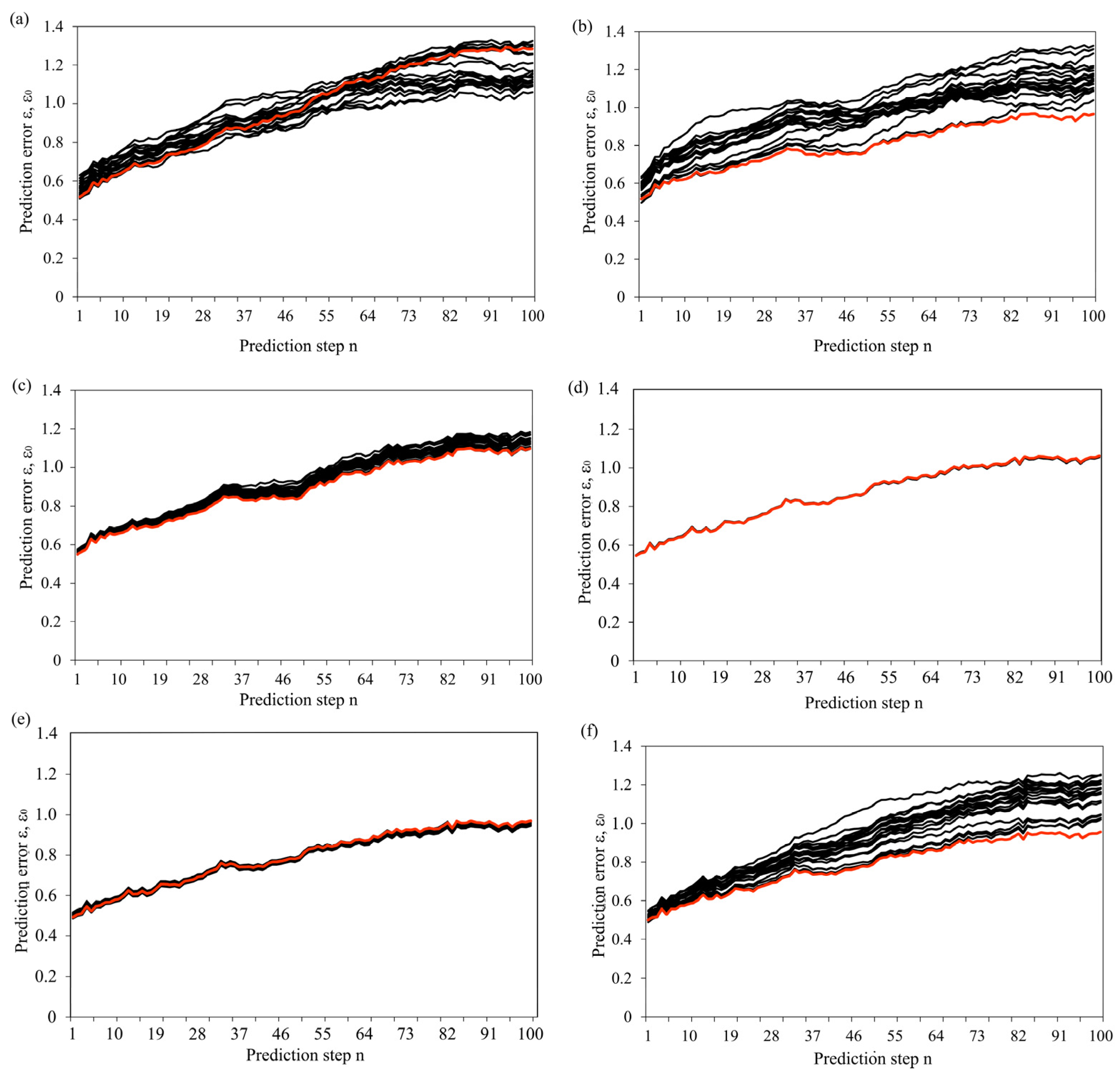
The results of surrogate data testing are given in Figure 3. In particular, we tested the first null hypothesis that data represent independent random numbers drawn from some fixed but unknown distribution. For this purpose, we formed 20 surrogate datasets by randomly shuffling the data (without repetition), thus yielding surrogates with exactly the same distribution yet independent construction and estimating zeroth-order prediction error for 100 prediction steps. It is clear from Figure 3 that prediction error ε0 for the original dataset is not within the prediction errors for all the tested surrogate datasets, ε, indicating that starting null hypothesis could be rejected.

As the second step in our analysis, we tested the null hypothesis that data represent a linear stationary stochastic process with Gaussian inputs. As in the previous case, we formed 20 surrogate datasets by randomizing the Fourier surrogates of the original data and then by computing the inverse transform to obtain randomized time series [23]. The results are shown in Figure 4. Obviously, we could not reject the null hypothesis (at a 95% significance level) since ε₀ is within ε for all the tested surrogates.

3. Effect of Noise on Landslide Dynamics

We assume that landslide dynamics could be modeled as the movement of the n interconnected blocks (Figure 5):

$$\begin{array}{c}d{x}_i\left(t\right)=y_i\left(t\right)dt\hfill \\ d{y}_i\left(t\right)=-\left[a{\left(V+y_i\left(t\right)\right)}^3-b{\left(V+y_i\left(t\right)\right)}^2+c\left(V+y_i\left(t\right)\right)\right]dt+\hfill \\ \hspace{1em}\hspace{1em}\hspace{1em}\hspace{1em}\hspace{1em} (a{V}^3-b{V}^2+cV)dt+{\sum }_{j=1}^N{k}_1\left(x_j\left(t-\tau \right)-x_i\left(t\right)\right)dt+\sqrt{2D}d{W}_i\hfill \end{array}$$

(1)

where x_i and y_i are displacement and velocity of the i-th block, respectively, k is the spring stiffness (could be considered to qualitatively correspond to the deformable properties of the surrounding soil), V is the background velocity, τ is a time delay in the position between two neighboring blocks, while a, b, and c are parameters of the cubic friction force, which according to Morales et al. [24] has the following form:

$$Fc\left(V\right)=3.2V^3-7.2V^2+4.8V$$

(2)

One should note that previous studies suggested that landslides exhibit frictional velocity-weakening [25,26]. Additionally, the assumed cubic friction law qualitatively corresponds to the Coulomb–Mohr nonlinear τ-u relationship.

Terms (2D)^1/2dW_i represent stochastic increments of the independent Wiener process, i.e., dW_i satisfy: E(dW_i) = 0, E (dW_idW_j) = δ_ijdt, where E() denotes the expectation over many realizations of the stochastic process and D is the intensity of additive local noise. In the present paper, we examine the effect of the persistent background seismic noise in order to determine whether this continuous factor has any effect on the landslide dynamics. The effect of noise on the stability of the model dynamics is examined through the effect of its intensity as the most important property of random noise.

It should be noted that the suggested model (1) represents a phenomenological model of landslide dynamics, with friction, displacement delay, spring stiffness, and random background noise as the main affecting factors. The effect of soil density is not explicitly included in the suggested model and could be considered constant for the purpose of the performed analysis.

One should note that model presented in Figure 5 is just an illustration; blocks within a model are globally (all-to-all) coupled. The idea of representing landslide dynamics as a dynamics of a spring-block model sliding down the slope came from Davis [27], and it was subsequently examined by Morales et al. [24]. Hence, model (1) is inspired by the original model by Davis [25] but with the explicitly included time delay and the effect of background noise. The combined effect of time delay and noise has been previously analyzed and reported as justified for different dynamical systems [28]. Additionally, some previous studies have indicated that vibrations could lead to frictional weakening [29].

We consider that the proposed model is close to natural conditions since it includes two main properties of the natural slope: delayed interaction among different parts of the slope and the influence of the background seismic noise. Adopted friction law, as shown in Equation (2), adequately mimics the cubic friction law existing along the potential (and real) sliding surface, with the natural transition from velocity strengthening to velocity weakening regime.

Equation (1) as a set of n stochastic delay differential equations is examined in the present paper using the mean-field approximation, by which one obtains the following mean-field model of the starting system (1):

$$\begin{array}{c}{\dot{m}}_x\left(t\right)=m_y\left(t\right)\hfill \\ {\dot{m}}_y\left(t\right)=\left(-3a{V}^2+2bV-c\right)m_y\left(t\right)+\left(b-3aV\right)\left(s_y\left(t\right)+m_y^2\left(t\right)\right)-a\left(m_y^3\left(t\right)+3m_y\left(t\right)s_y\left(t\right)\right)\hfill \\ \frac{1}{2}{\dot{s}}_x\left(t\right)=U(t)\hfill \\ \frac{1}{2}{\dot{s}}_y\left(t\right)=s_y\left(t\right)\left[\left(2bV-3a{V}^2-c\right)+2\left(b-3aV\right)m_y\left(t\right)-3a\left(m_y^2\left(t\right)+s_y\left(t\right)\right)\right]-kU\left(t\right)+D\hfill \\ \dot{U}\left(t\right)=U\left(t\right)\left[\left(2bV-3a{V}^2-c\right)+2\left(b-3aV\right)m_y\left(t\right)-3a(s_y\left(t\right)+m_y^2\left(t\right))\right]+s_y\left(t\right)-k{s}_x(t)\hfill \end{array}$$

(3)

where the first and second-order cumulants are denoted in the following way: (a) the means $m_x\left(t\right)=〈x\left(t\right)〉,m_x\left(t-\tau \right)=〈x(t-\tau )〉,m_y\left(t\right)=〈y\left(t\right)〉$, (b) the mean square deviations $s_x\left(t\right)=〈n_x^2\left(t\right)〉,s_y\left(t\right)=〈n_y^2\left(t\right)〉$ and (c) the cross-cumulant $U\left(t\right)=〈n_x{n}_y〉$. Noise intensity is denoted with D, V stands for the block velocity, while a, b, and c denote cubic friction parameters.

Details of the derivation of model (3) are given in Appendix A. The justification for reducing the model of n units to a single mean-field model lies in the very nature of the specific landslide “Zavoj” itself, for which the recorded background seismic noise was also examined. In particular, the whole landslide body is composed of the weathered bedrock material (Figure 6), whose dynamics, therefore, could be analyzed as the behavior of the reduced mean-field model. Moreover, in the present paper, we are interested in the global stability of the landslide model. This is why we seek the transition between the global dynamical regimes, while small dynamical effects that may occur due to the dynamics of individual blocks are not of interest in the present paper.

The analysis of the influence of random background noise on the dynamics of the landslide model (3) is conducted numerically, using the 4th order Runge–Kutta numerical method, under the effect of the introduced time delay τ and spring stiffness k. Results of the conducted analysis indicate the occurrence of the direct supercritical Hopf bifurcation, with an increase in time delay and/or spring stiffness (Figure 7). Particularly, the observed dynamical system goes from an equilibrium state (represented as small constant background displacement, the so-called “creep regime”) to regular periodic oscillations, which are considered unstable dynamical regimes. The trend of the bifurcation curve indicates the following: for the higher values of spring stiffness (or the low-deformable slopes), only the small values of displacement delay are required to trigger the instability. On the other hand, for low values of spring stiffness (high-deformable slopes), the increase of displacement delay has de facto no effect on the stability of the examined model.

One can easily show that the dynamics of the starting stochastic model (1) and the mean-field model (3) before and after the bifurcation curve are qualitatively similar, as it is shown in Figure 8. The first row shows the mean velocity of the starting stochastic system (1), Figure 8a, and the mean of the deterministic mean-field model (3), Figure 8b, before the bifurcation curve shown in Figure 7, for k = 10 and τ = 1 (point a). It is clear that both systems are in an equilibrium state. The second row shows the mean velocity of the starting stochastic system (1), Figure 8c, and the mean of the deterministic mean-field model (3), Figure 8d, after the bifurcation curve shown in Figure 7, for k = 10 and τ = 3 (point b). Both systems exhibit periodic oscillations.

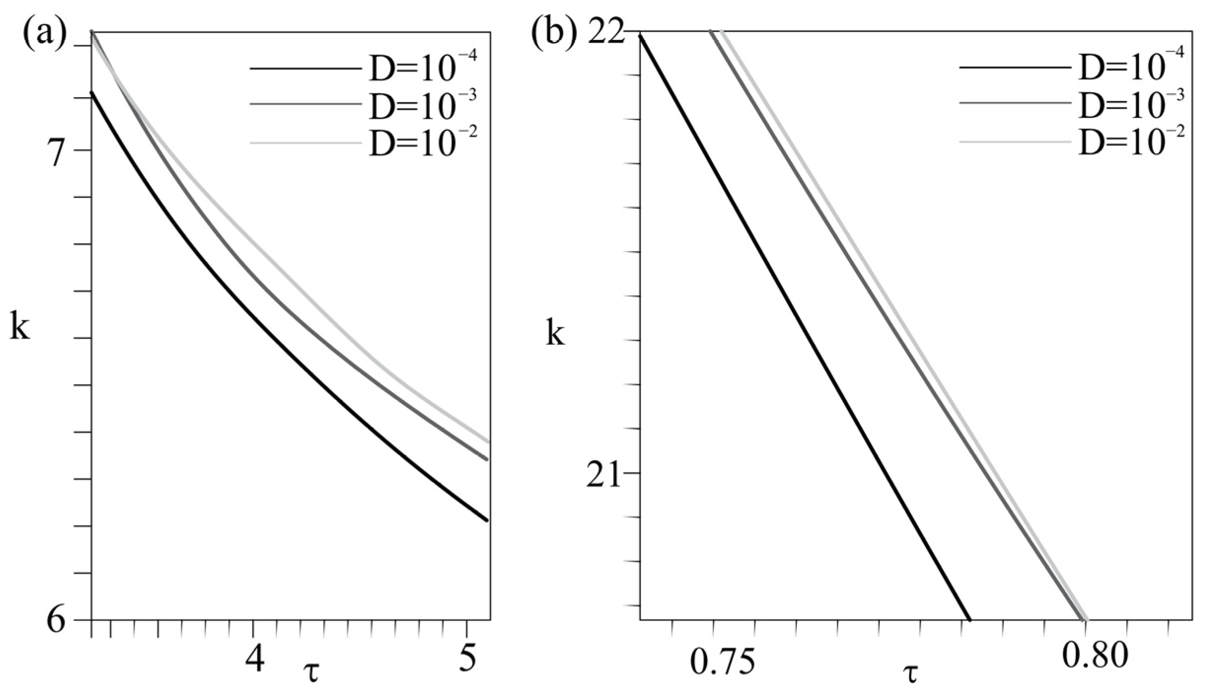
Regarding the effect of noise on landslide dynamics, further analyses imply the following. Figure 9 shows the effect of different noise intensities on the position of the bifurcation curve in the k-τ diagram. Landslide dynamics before the bifurcation curves are considered to be stable (creeping state), while landslide dynamics after the bifurcation curves are considered to be unstable. It seems there is a positive effect of random background noise on landslide stability. In particular, with the increase of the intensity of random noise from 10⁻⁴ to 10⁻², the Hopf bifurcation curve ”moves” further, i.e., higher values of time delay or spring stiffness are needed for the instability to occur. This effect is pronounced both for the low and high values of time delay and spring stiffness, as shown in Figure 9. Such an effect for high values of time delay (3.5–5.0) and relatively low values of spring stiffness is shown in Figure 9a. These conditions are expected in strongly weathered rock masses, with loose connections between the actual moving parts of the unstable slope, where higher values of delayed interactions are expected. It is clearly seen that for constant spring stiffness and time delay, solely by increasing the noise intensity, the system under study becomes stable. The effect of noise for low values of time delay (0.75–0.80) and high values of spring stiffness is shown in Figure 9b. Such a regime corresponds to rock mass which is just slightly weathered with low deformability, where low values of delayed interaction are expected. One could see that increase of D for constant k and τ leads to the stabilization of landslide dynamics. Additionally, vice versa, the reduction of D destabilizes the dynamics of the landslide. Moreover, this effect is pronounced between 10⁻⁴ and 10⁻³, while the further effect of D is significantly lower. This is a rather unexpected result implying a positive role of noise on slope stability compared to the influence of delay interaction or coupling stiffness.

4. Discussion and Conclusions

In the present paper, we propose a landslide model that includes delayed interaction and the effect of random background noise. In the first phase of the paper, the introduction of background seismic noise is justified by the results of the analysis of the monitored ambient noise within the location of the existing landslide in Serbia. The analysis is conducted using surrogate data testing and results in a classification of the analyzed monitoring results as linear stationary stochastic processes with Gaussian inputs. This justified the introduction of background random noise in the dynamical system proposed in the present paper. The model is suggested in the form of stochastic delay-differential equations, with included effect of delayed interaction and background seismic noise. Friction is assumed to be rate-dependent which is very well aligned with the results of previous studies. The dynamics of the proposed dynamical system are examined using mean-filed approximation: the derived mean-field model is shown to exhibit qualitatively the same dynamics as the starting stochastic model. The justification for using a single mean-field model instead of n globally coupled stochastic units lies in the very nature of the landslides formed in weathered rock mass: dynamics of such landslides could be observed as the average dynamics of the whole slope.

Results of the conducted numerical analyses indicated that with the increase of spring stiffness and time delay, a direct Hopf supercritical bifurcation occurs, with the transition from a creeping state (constant displacement of low intensity) to regular periodic oscillations (unstable regime).

The effect of noise on the dynamics of the suggested model is examined further numerically. It is shown that background noise has a positive effect on the stability of the landslide dynamics. In particular, noise has the same effect for highly weathered rock masses, with rather low values of spring stiffness and high values of time delay, and for slightly weathered rock masses, with high values of spring stiffness and low values of time delay. In both cases, an increase of D ”stabilizes” the landslide, and vice versa—reduction of noise leads to the onset of slope instability. Such a stabilizing effect of the background noise confirms the significance of its effect, particularly near the bifurcation point, which is valid for the creeping landslides.

From the geodynamical viewpoint, the obtained results could be interpreted in the following way:

• Creeping slopes composed of highly weathered rocks, where individual unstable parts have loose interaction with high delay, are sensitive to the change of the background noise intensity. In this case, the interaction of time delay and noise intensity is particularly emphasized: an increase of noise intensity for two units of order leads to the significant stabilization of landslide activity, with the increase of time delay for 1. The interaction of noise and spring stiffness is not so significant, and approximately one order of units is smaller compared to the interaction of noise and time delay. In particular, an increase of noise intensity for two orders of units leads to the change in critical values of spring stiffness for approximately 0.1.
• Creeping landslides composed of slightly weathered rock masses, where individual unstable parts have strong interactions, with low values of time delay, are more sensitive to the interaction of delay and spring stiffness compared to the interaction of D and τ. With the increase of D for two orders of units, critical values of k (for which bifurcation occurs) change by approximately 0.5, while the critical value of τ changes by approximately 0.03.

We consider that there are several main novelties of our research: (1) we confirm the existence and type of background ambient noise before and after the small seismic events in a landslide-prone area, (2) we suggest a new model for landslide dynamics with the included effect of the random background noise, (3) our results indicate a significant effect of the noise on landslide dynamics when the landslide is in a critical state (right before the bifurcation point), and (4) our results indicate a positive, stabilizing effect of noise on landslide dynamics.

Present research on this topic could further include the analysis of the possible significant effect of random noise in interaction with different friction parameters. Additionally, the possible significant effect of the colored noise of various origins could be further examined.