Article

Mixed-Integer Linear Programming, Constraint Programming and a Novel Dedicated Heuristic for Production Scheduling in a Packaging Plant

1
Brodart SAS, 1 Rue du Stand, 10700 Arcis-sur-Aube, France
2
Laboratory of Computer Science and Digital Society (LIST3N), University of Technology of Troyes, 12 Rue Marie Curie, CS42060, 10004 Troyes Cedex, France
*
Authors to whom correspondence should be addressed.
Appl. Sci. 2023, 13(10), 6003; https://doi.org/10.3390/app13106003
Submission received: 14 April 2023 / Revised: 10 May 2023 / Accepted: 10 May 2023 / Published: 13 May 2023
(This article belongs to the Special Issue Design and Optimization of Manufacturing Systems)

Abstract

:
In this paper, we are discussing a research project aiming to optimize the scheduling of production orders within a real application in the packaging field. As a first approach, we model the problem as an extended version of the hybrid and flexible flowshop scheduling problem with precedence constraints, parallel machines, and sequence-dependent setups. The optimization objective considered is the minimization of the total tardiness. To tackle this problem, we use two methodologies: mixed-integer linear programming (MILP) and constraint programming (CP). These two models were further extended by adding resource calendar constraints named also availability constraints; this implies that the tasks should be scheduled only when the machine is available. The different proposed models were compared to each other on a set of generated benchmarks that reflect the specific properties of the industrial partner. Finally, as the studied configuration relies on practical real-world application, where thousands of orders are produced monthly, a novel dedicated heuristic was designed to address the need for quick solutions. The latter outperforms the other proposed algorithms for expected total tardiness minimization. The proposed problem can be readily modified to suit a wide range of real-world situations involving the scheduling of activities that share similar characteristics.

1. Introduction

Effective production planning and scheduling attract continuous interest from manufacturing companies, which is a good way to add flexibility to the business, to meet the deadlines promised to the customer, and to ensure the best production efficiency by balancing production needs with available resources, all at minimal cost. From this point of view, the use of robust tools for production scheduling remains a strategic issue because they enable optimizing production and meeting market challenges.
Scheduling is the operational organization of production in the workshop by deciding the order in which tasks pass through the machines, respecting a certain number of constraints to which the workshop is subjected, and according to optimization criteria considered for decision making. In other words, the schedule can be defined as follows: assign the task ‘ i ’ to the machine ‘ k ’ at a given time ‘ t ’ while considering, for example, the operator ‘ p ’ equipped with the tool ‘ o ’ and the mater ‘ m ’.
Among different workshop configurations, a flowshop scheduling problem (FS) arises in the context of repeated production, where jobs are required to visit the stages in the same order and undergo identical processing operations; in other words, all operations of all tasks go through the machines in the same order. In order to cope with real-world problems, improve the overall capacity, add additional flexibility to the production, and avoid bottlenecks if some operations are too long, it is possible to multiply the number of machines that can perform the same operation. The resulting model is known in the literature as hybrid flowshop (HFS), also called flowshop with parallel machines; it consists of a set of processing stages, in which each stage may have several identical or non-identical machines, with at least one stage having two or more parallel machines. The classical hybrid flowshop assumes that all jobs need to visit all stages in the same order. However, in practice, each job might miss out or skip some stages, which can improve the performance of the model and make it better suited for real-world industrial settings. HFS scheduling problem with stage skipping is also called hybrid flexible flowshop scheduling problem. The configuration under study is described in Figure 1.
In hybrid and flexible flowshop (HFFS) scheduling problems, two decisions should be taken: the assignment of jobs to the parallel machines as well as the sequencing of the jobs allocated to each machine. This problem is known to be NPhard in its simple version and in most of its extensions. As an example, Hoogever et al. [1] demonstrated that preemptive scheduling in a two-stage flowshop with at least two identical parallel machines in one of the stages so as to minimize makespan is NP-hard in the strong sense. Gupta et al. [2] considered a non-preemptive two-stage hybrid flowshop problem in which the first stage contains several identical machines and the second stage contains a single machine; they demonstrated that the problem is NP-hard in the strong sense even when there are only two machines at the first stage. HFFS scheduling problem has been widely applied in various manufacturing environments, and several realistic constraints were considered. A fair amount of research has focused on a variety of realistic constraints, ranging from sequence-dependent setup times, constraint calendar, transportation time, due dates, and so on. Furthermore, several optimization criteria were considered, covering the commonly used makespan, costs, transportation, maximum tardiness and earliness, and the total of tardy job.
In this paper, we make three significant contributions. Firstly, we introduce novel CP and MILP models that take into account specific constraints, including sequence-dependent setups and resource calendar constraints. Secondly, we assess the performance of both models using real industrial benchmarks. Lastly, we propose a dedicated heuristic that effectively addresses the need for fast computation times in practical real-world applications, such as the one studied in this paper, where thousands of orders are produced each month.
The remainder of this paper is organized as follows: Section 2 reviews the state of the art regarding the related papers. The problem description is presented in Section 3. In Section 4, we formulate all the proposed resolution models (MILP, CP, and a novel dedicated heuristic). The computational experiments, allowing to evaluate the performance of the proposed models, are presented in Section 5. Finally, in Section 6, we present the conclusions of our work.

2. State of the Art

The area of flowshop scheduling has been a very active field of research. It was first proposed by Johnson in 1954. Since then, several approaches have been proposed and numerous optimization objectives were considered. The current trends that attracted researchers during the last decade in scheduling problems are toward integrating practical constraints. Among all, we can point out setup time, resource calendar, and machine flexibility.

2.1. Constraints

2.1.1. Setup Constraints

Setup time, also called changeover, is a very important factor in the packaging industry because it may have a significant impact on the overall production cycle. It denotes the required time interval to prepare the necessary material resources. In many real-life situations, a setup often occurs while shifting from one operation to another. Setup time is classified into two categories: sequence-independent setup time and sequence-dependent setup time. Sequence-independent setup time depends solely on the current task regardless of its previous task. Sequence-dependent setup time depends on both the current and immediately preceding task [3,4].
There has been a growth in interest in incorporating setup times in many studies. The main reason why researchers have been motivated to utilize this assumption is to solve scheduling problems in a real manner [5] Liu and Chang [6] addressed the problem of F m | S t s d , C s d , r i | S T i , C i . They first formulated the problem as an integer programming problem. Then, they employed a Lagrangian relaxation approach and finally developed a search heuristic. Three major types of heuristics were proposed by Kurz and Askin [7], who explored the F m | S t s d , C s d , r i | C i problem, namely insertion heuristics (based on insertion heuristics for the traveling salesman problem), Johnson’s algorithm, and a set of naïve greedy heuristics. They investigated these three patterns and identified the range of conditions under which each method performs well. Salmasi et al. [8] proposed a mathematical programming model for F m | f m l s , S t s d | C i as the problem is proven to be strongly NP-hard; two heuristic algorithms, tabu search (TS) and hybrid ant colony optimization (HACO), were developed to solve the problem. In addition, a lower bounding method based on the branch and price algorithm was developed to assess the performance of the metaheuristic algorithms. An et al. [9] considered the F 2 | w t , S t s d | C m a x problem; they developed several dominance properties, lower bounds, and heuristic algorithms and used the latter to develop an efficient branch and bound algorithm. Cheng et al. [10] tackled the F p | S t s d | C m a x problem; they proposed a mixed-integer linear programming model to solve small-sized instances. Due to the strong NP hardness of the research problem, an effective metaheuristic, called pairwise iterated greedy (PIG) algorithm, was proposed to solve medium- and large-sized problems. Rossi and Nagano [11] proposed a mixed-integer linear programming (MILP) model for F m | S t s d | T i problem. They proposed a method to evaluate the total tardiness of a permutation sequence and also introduced a partial acceleration method to calculate the total tardiness in an insertion neighborhood. In addition, they developed a new heuristic to solve the problem efficiently. This heuristic was then integrated into the best metaheuristics available in the literature. Kare and Agrawal [12] studied the F m S t s d w T i , w E i problem. Three evolutionary metaheuristics were proposed.

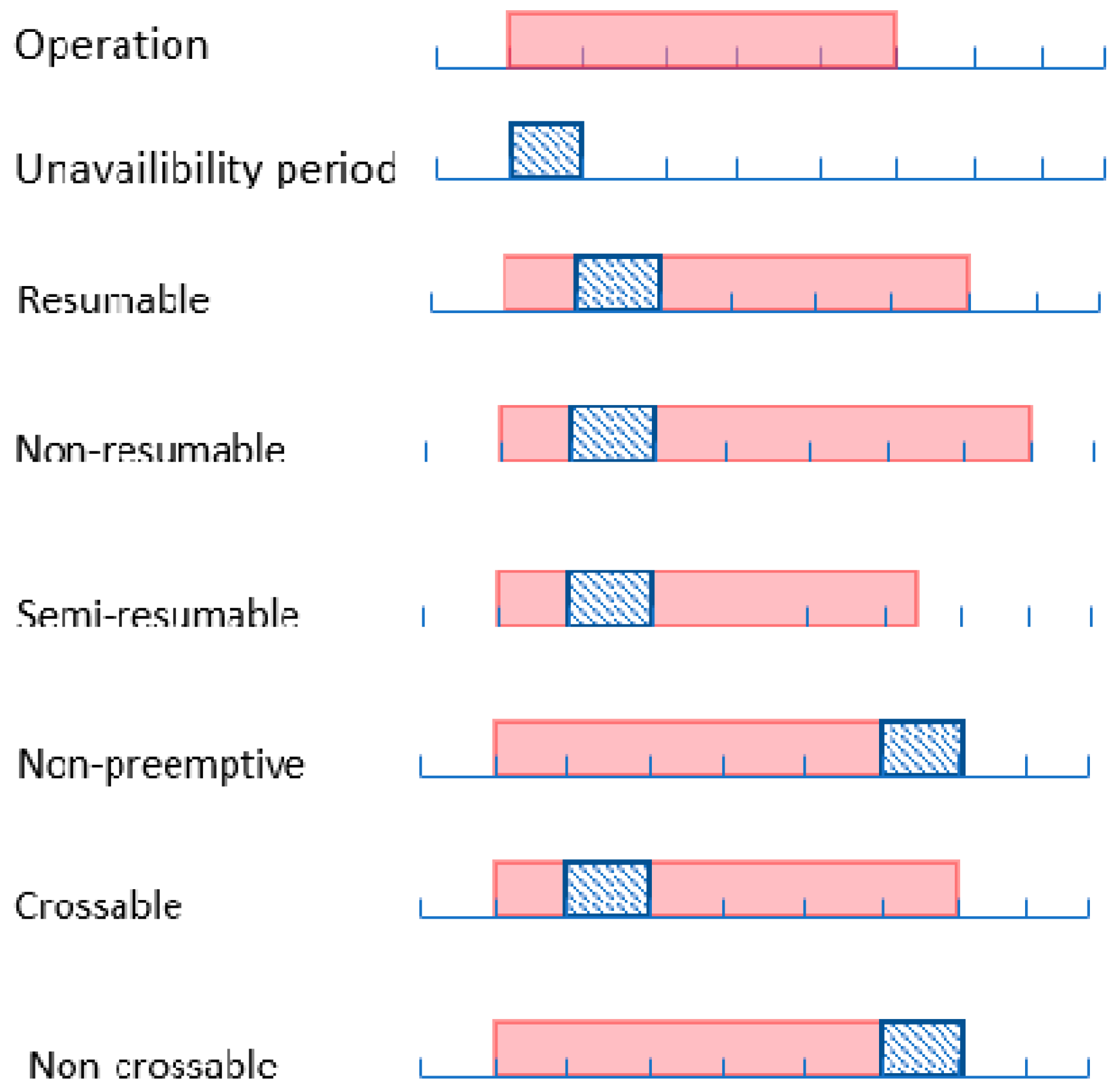
2.1.2. Resource Calendar Constraints

Another common and practical constraint found in real environments is to consider the resource calendar. The traditional scheduling problem assumes that machines are continuously available. However, in reality, this is often not the case due to non-availability periods, such as maintenance, vacations, leaves, and so on. Considering these time-off periods for resources is crucial for accurate and realistic scheduling. This helps to determine when resources are available to work on assigned tasks, ensuring that work is only scheduled during available times.
Machine availability constraints encountered in real-world environments can be classified as either fixed or non-fixed [13]. For fixed constraints, the intervals of unavailability are predetermined, whereas they are unknown for the non-fixed constraints. Unavailability periods can also be categorized based on operation preemption as non-preemptive [14], crossable or non-crossable [15], or resumable, semi-resumable, or non-resumable [16]. An operation is known as non-preemptive when its processing on a machine cannot be interrupted until it is totally completed, and after that the concerning machine switches to another operation. An operation interrupted by an unavailability period is called resumable when its processing can continue during the next availability period. It is called non-resumable if it has to restart from the beginning when the performing machine is available again. An operation is known as semi-resumable if it has to partially restart during the next available period. There is other terminology introduced by Mauguière et al. [15]. It concerns unavailability periods allowing interruption of operations: crossable and non-crossable unavailability periods. An unavailability period that allows an operation to be interrupted and resumed after the unavailability period is called crossable, while an unavailability period that does not allow the interruption of any operation is known as non-crossable. Figure 2 gives a description for the notation used for interruptible and non-interruptible operations.
Bentalleb et al. [17] consider a deterministic case where unavailability periods are known in advance and fixed and correspond to preventive maintenance tasks. They tackled a two-machine job shop scheduling problem with an availability constraint on one machine under makespan minimization. First, two mixed-integer programming (MIP) models were proposed and then some heuristics were performed to solve the problem. Azem et al. [18] investigate the job shop problem where operations can be interrupted by resource unavailability periods. They propose approximation methods based on construction heuristics.
Surprisingly, the literature on the flowshop scheduling problems with resource calendar or fixed machine availability is not abundant. Aggoune et al. [14] address the flowshop scheduling problem with limited machine availability under the makespan criterion and under the assumption that the machines are not available during the whole planning horizon. They propose a heuristic approach based on the geometric approach to approximately solve the problem. Figealska [19] studied the problem of preemptive scheduling in a two-stage flowshop with parallel unrelated machines under makespan minimization. Heuristic algorithms were proposed based on combined linear programming procedures and a genetic algorithm. Laribi et al. [20] investigate an extension of the classical flowshop scheduling problem to the case where jobs processing requires additional nonrenewable resources; the goal is to minimize the makespan. They propose an efficient mathematical model.

2.1.3. Machine Flexibility Constraints

In a modern manufacturing unit, machine flexibility is a very important feature that enables increasing the overall workshop capacities, reducing or eliminating the impact of bottleneck stages and balancing the capacities of the stages for the overall workshop. Such a production unit is characterized by several stages. Each stage is made up of a set of parallel machines. At some stages, the machines are duplicated and a job can be processed on any machine. A flowshop with parallel machines is also known as a multiprocessor flowshop, flexible flowshop, or hybrid flowshop. Machine flexibility has attracted much attention from researchers in recent years. There are several examples provided in the literature, including steelmaking [21,22], industry [23], as well as the semiconductor industry [24,25]. Odugawa et al. [26] provide a survey on several real-world applications, ranging from the metal forming industry to the paper industry to the chemical industry. Some researchers address real-world problems in their papers.
Kochhar et al. [27] exhibit a local search approach to solve highly realistic flexible flow line scheduling with setups, buffer capacities, as well as blocking and breakdowns. Several heuristics are provided by Botta-Genoulaz [28] for the flowshop scheduling problem with multiple identical machines per stage, precedence constraints and time lags, and setups. Ruiz and Maroto [29] provide a metaheuristic, in the form of a genetic algorithm, to a complex generalized flowshop scheduling problem that results from the addition of unrelated parallel machines at each stage, sequence-dependent setup times, as well as machine eligibility. Naderi et al. [30] investigate the problem of hybrid flexible flowshop (HFFS) with sequence-dependent setups, where the objective is to minimize the makespan. They put forward two advanced algorithms that effectively handle the flexible and setup features of this problem. Chen [31] proposed an integer hybrid metaheuristic based on the principles of variable-neighborhood descent and TS for unrelated parallel machines problems with ready times and sequence- and machine-dependent setup times to minimize the weighted number of tardy jobs.
While many papers in the literature have tackled various realistic considerations and constraints, to the best of our knowledge, there has been no effort to jointly address the set of realistic constraints incorporated in the problem formulation of our paper, which include sequence-dependent setups, machine flexibility, and resource calendar constraints.

2.2. Optimization Criteria

Setting the correct optimization criteria or objectives for a scheduling problem is not always an easy task as they are diverse, convoluted, and often conflicting. Plenty of scheduling problems have been studied considering several criteria. The most considered are makespan ( C m a x ), total flow time, total tardiness, maximum tardiness, and number of tardy jobs. Makespan and total flow time seek the effective utilization of the manufacturing resources by reducing the elapsed time between the start and the completion of a sequence of operations in a set of machines, while the remaining criteria are related to job due dates. In fact, makespan minimization is significantly important in order to upsurge the utilization of the production system. However, in today’s competitive environment, focusing on makespan minimization without meeting the due date is of no use for an industry since meeting customer deadlines is crucial. According to Sen and Gupta [32], when a task is not completed before its due date, some penalties are incurred, such as potential loss of customers, damaged reputation, loss of market competitiveness, penalty clauses if there are any, as well as expediting (the job is assigned quickly to the processing machine at the possible cost of extra setups, double handling of material, inefficient use of workmen and machine), etc. Hence, scheduling problems with tardiness objectives have attracted increasing attention from managers and researchers. Table 1 provides a summary of several significant studies that focus on the tardiness objective. The “Constraints” column contains the various constraints that were taken into account in these studies. The “//m” column refers to parallel machines, the “ S T s d ” column pertains to sequence-dependent setups, the “ d i ” column represents due date constraints, the “ w i ” column represents waiting time, and finally the “ r i ” column represents release date constraints.

3. Problem Description

The problem under study corresponds to a real industrial problem of a packaging company that prints, on average, 1000 jobs per month. The operations can be categorized into four main groups, ranging from the preparation of printing materials to the printing process and shifting process (winding, perforation, and coating) and finally shaping process aiming to make orders into their final form. Moreover, it is important to point out that this process is characterized by flexibility, where machines might be skipped and not all the machines must be visited by all the jobs.
A job i consists of a number n of operations; each operation O i j can be processed by a subset of machines and has a processing time on machine k , and it may be zero for some jobs as the jobs are not processed in some stages (skipping). Note that p i denotes the processing time of job i .
Before starting processing, a setup time (ST) is needed between each of two consecutive scheduled jobs on each machine. That is to say that, to transition from the processing of the current operation O i j to the next one O i j on machine k , some setup settings must be implemented according to the characteristics of each operation, such as color, size, etc. An example of setup for the printing phase consists of removing the ink colors not required for the next job on that printing machine to free up the ink trays for colors that are required for the next job. Transitioning from one job to another requires to change ink colors. The time required to set up one job for the printing phase can be divided into three steps: the first one to empty the tray from the previous ink, the second one to clean the ink tray, and the last one to reload the appropriate ink color. The global needed setup time depends on the number of color changes. On average, the significant setups may contribute to 40% of the global printing step, including processing time and setup time. However, if a job i requires the same color as the previous job i 1 , then the setup time for this color may be avoided because the considered printing machine is already loaded with appropriate color and, therefore, major setups are not needed. The setup time duration is correlated to the setup settings’ similarities between two consecutive operations. The more resemblance the operations’ settings, the shorter the machine setup.
Another important feature of the considered problem is resource calendar constraints (RC), which allow to set the work shifts of all machines. The work shift is a segment of continuous available times of a machine. This means that machines are available only during working times in the calendar. These unavailability periods are the consequence of shift patterns or planned maintenance. On the other hand, the machine setup cannot be interrupted by unavailable periods, and the end of the setup must be immediately followed by the beginning of the operation processing. Furthermore, a transportation time is needed to transport a job from the current processing machine to the next one.
Based on the key features of the considered production system, a production schedule should be planned to maximize the production effectiveness so that the printing line can gain as much production benefit as possible. The production effectiveness can be represented by an objective function that should be defined based on the production targets of the problem. In flexible manufacturing plants operating in a make-to-order environment, the efficient utilization of manufacturing resources is typically pursued to meet delivery deadlines. Thus, in our case, we aim to minimize the total tardiness of all jobs, meaning that we seek to find a job sequence that minimizes the total amount of time by which all jobs are completed after their due dates.
The production problem can be described as a hybrid and flexible flowshop with nineteen unrelated parallel machines, denoted using the classical Graham notation H F F 19 | P r e c , S T s d , R C , d i | j = 1 n t i [56]. This classification is based on the features mentioned above, and it is commonly used to represent production systems.
As the first systematic attempt to solve this problem, we construct a mathematical model in the form of mixed-integer linear program (MILP) that considers sequence-dependent setups; we then add waiting constraints and evaluate how it behaves, and, finally, we added resource calendar constraints that enhanced the complexity of the problem. The objective is to both assign jobs to one machine at each stage and then sequence jobs on machines to minimize the total tardiness.
If the completion time of a job is greater than its due date ( C i > d i ) , then it is called tardy and tardiness takes positive values. Otherwise, it becomes an early job with a tardiness value equal to zero ( t i = m a x ( 0 , C i d i )).

4. Model and Notations

Job characteristics are modeled as follows:
Let N be the number of jobs to be scheduled. Each job i ( i = 1 N ) is composed of a set of operations J i that must be processed according the defined processing route. Let M be the number of all available material resources “machines”. For each operation j , let m j M be the set of operations that can perform j j i and p i k be the corresponding processing times.
To transition from executing operation Oij to operation Oi’j’ on machine k, a setup time s t i j i j k must be incurred. In our problem, the setup time for a job is dependent on the previous job that was processed on the same machine and thus on the job processing sequence. For each machine K k = 1 m , let l k be the number of unavailability periods and υ k l , υ k l the time window of unavailability of material resource k m . The processing of each job on the latter can only be preempted by this interval υ k l , υ k l and resumed once the machine becomes available. Let d i denote the due date and specify the time limit by which job i N should be completed. The number of jobs, their respective processing times, and due dates are predetermined and known beforehand. Each machine has a capacity and can only process one job at a time. A machine can only process one operation at a time. The processing of the latter can be interrupted by an unavailability period. Setups cannot be interrupted by an unavailability period and should occur when the machine is available during the setup interval, and, once completed, the processing of the associated operation should start. There is no limit on the capacity of the intermediate stock (buffer) between the production stages. Finally, the objective is to minimize the total tardiness.
The notation used in this mathematical modelling is summarized in Table 2 and Table 3:

4.1. Mixed-Integer Linear Programming

In this section, the MILP formulation presented in [3] is recalled using the notation of Section 4 and afterwards extended in Section 4.1.2 by adding resource calendar constraints.

4.1.1. Start-Based Model

The start-based model was developed in our previous work [3], with the consideration of sequence-dependent setups, parallel machines, and precedence constraints, and this model is formulated as a mixed-integer linear programming model as below and called M I L P w a v from now on.
M i n i m i z e   T = i = 1 n t i
Subject to:
t i = max ( C i d i )
k = 1 m e X i j k = 1 , i N , j J i , k m j
C i j k S i j k + P i j k B i g M ( 1 X i j k ) , i N , j J i , k m j
S i j k + C i j k B i g M ( X i j k ) , i N , j J i , k m j
C i j k   S i j k , i N , j J i , k m j
i j j , j o i k m i Y i j i j k = 1 , i , i N , j , j J i , J i k m i j m i j
S i j k C i j k + S t i j i j k B i g M ( 1 Y i j i j k ) , i , i N , j , j J i , J i k m i j m i j
S i j k C i j k + S t i j i j k B i g M Y i j i j k , i , i N , j , j , J i , J i , k m i j m i j
C i j k = P i j k + S i j k , i N , j J i , k m j
C i = k = 1 m i j C i j k , i N , j J i , k m i j
t i 0 , i N
X i j k { 0,1 } ; i N , j o i , m i j
Y i j i j k 0,1 , i , i N , j J i , j J i , k m i j m i j
S i j k 0 , i N , j J i , k m i j
C i j k 0 , i N , j J i , k m i j
The objective function (1) aims at minimizing the sum of the total tardiness of all jobs. Constraint (2) provide us with the value of the individual tardiness of each job. Constraint (3) states that each operation can only be assigned to one machine, where the decision variable X i j k is non-zero if operation Oij is assigned to processing unit k and zero otherwise. Constraint (4) ensures that a job’s completion time is no earlier than the sum of its start time and processing time. Constraint (5) sets the end date of each job on machines that are not processing the job to 0. Constraint set (6) controls job completion at stages that a job may skip. Constraint set (7) enforces precedence constraints, ensuring that each operation of a job can only begin after its preceding operation has been completed. Constraints (8) and (9) are used together to sequence any pair of tasks (i, i′) assigned to the same processing unit k, preventing two jobs from being processed simultaneously on the same machine to ensure the machine is occupied when processing an operation. Constraint set (10) specifies that the completion time of any operation is the sum of its start time and processing time. Constraint set (11) calculates the completion time of a job as the sum of the completion times of all the operations in its processing route. Constraint (12) ensures that only positive tardiness values are considered. Finally, Constraint sets (13) (14), (15), and (16) define the decision variable domains.

4.1.2. Modeling Calendar Constraints

The start-based model is further extended to solve unavailability problems, which are also addressed by incorporating resource calendar constraints. The processing of a job should not start during the time window of unavailability of resource k. That is to say that any operation must be carried out and finished before the arrival of an interval of unavailability. The execution time of an operation must be outside unavailability interval.
S i j k , S i j k + P i j k υ k l , υ k l =
Constraint (18) allows to calculate the total unavailability period of a machine k that processes job i.
u i = k = m l l k X i k ( υ k l υ k l )
Constraint (19) calculates the operations completion time
C i j k = P i j k + S i j k + S t i j i j k + u i , i N , j J i , k m j
Now, we have:
C i = k = 1 m i P i j k + S i j k + S t i j i j k + u i , i N
From now on, we refer to the model that incorporates resource calendar constraints into model M I L P w a v , M I L P R C .

4.2. Constraint Programming

Constraint programming (CP) has good performance and robustness in the optimization field. In fact, it is a strong tool for solving discrete optimization problems; it provides a set of modeling features suitable for a very wide range of complex scheduling problems that do not have a simple formulation. It provides an algebraic language with simple mathematical concepts; commonly, CP framework contains useful structural information; it has the advantage of exposing high declarative, compact, and flexible constraint formulations, which allow us to model the problem correctly and therefore makes it perform well for finding optimal feasible solutions [4].
Here, we have modeled the problem in CP using IBM ILOG CP Optimizer. We will not provide the details of the modeling language used in this paper. For those interested in learning more about this, we recommend referring to [57] and the CP Optimizer reference manual.

4.2.1. Start-Based CP Model

A formulation of the main variables is presented in Table 4 using the concepts of CP Optimizer. From now on, this model is called C P w a v .
Minimize   T = i = 1 n m a x ( 0 , t i )
Subject to:
t i = m a x ( 0 , e n d O f ( i t v s [ C i ] ) d i )
EndBeforeStart   ( β j ,   [ α j k ] ) j J i ,   k m i
Alternative   ( β j β j ) j , j J i
n o O v e r l a p [ α j k ] j J , k m j
d i β i . e n d   i N
i n t e r v a l   α j k , o p t , s i z e = P j k + S t j j k , i V , k m i
e n d A t S t a r t ( S t j j k , α j k ) j J , k m j
The objective function is to minimize the total tardiness (21), given by the difference between the job’s end value and due date (22). The EndBeforeStart constraints (23) represent the precedence constraints between interval variables. Alternative constraints (24) represent the assignment constraints stating that each operation must be performed on exactly one machine. Constraint (25) defines the nonoverlapping constraint; that is to say that, during the interval [ α j k ] , which represents the assignment of an operation j to machine k, the latter cannot overlap; e.g., the machine is busy during this interval.
The constraint endAtStart (α, β) is used to state that the end of a given interval variable α, equals the start of a given interval variable β. We use this constraint (28) to ensure that the end of a setup should be followed by the execution of the considered operation.

4.2.2. Modeling Calendar Constraints

The considered processing line is periodically submitted to calendar constraints; this means that machines are not available during the whole planning horizon. To consider machines’ unavailability, variable α j k should be modulated by adding an intensity step function F k that represents the unavailability interval of machine k. In CP optimizer, Intensity is a stepwise function that applies a measure of usage or utility over an interval length. The intensity is 0% during the unavailability interval υ k l , υ k l and 100% outside this interval. Therefore, modelling machines’ unavailability can simply be formulated by constraint (29)
i n t e r v a l   α j k , o p t , s i z e = P j k , i n t e s i t y = F k , j J , k m j
An additional feature of our problem is that the setup cannot occur during an unavailability period. To model this feature, we use the predefined constraint forbidExtent (a,U). This expression prevents an interval variable from being scheduled during any time point within the augmented horizon that is not also within one of the disjoint time windows.
f o r b i d E x t e n t S t i i k , F k , i , i N , k m i
Forbidden start constraint f o r b i d S t a r t α , F states that, whenever the interval is present, it cannot start at a value t where F t = 0 . In the same sense, Forbidden end constraint f o r b i d E n d α , F states that, whenever the interval is present, it cannot end at a value t where F t 1 = 0 . We use constraints (31) and (2) to ensure the respect of unavailability periods.
f o r b i d S t a r t α j k , F k , j J , k m i
f o r b i d E n d α j k , F k , j J , k m i
From now on, we refer to the model that incorporates resource calendar constraints into model C P w a v , C P R C .

4.3. Dedicated Heuristic

In order to meet the needs of an industrial environment, we need to be able to develop quick and effective solutions that can be used to solve the various tasks that are involved for a real industrial framework. Unfortunately, the exact resolution approaches presented previously cannot sufficiently address the requirements for real industrial-size instances (more than 100 tasks). A very common difficulty when trying to solve such large-sized instances with the MILP model is running out of memory. The CP model reaches better solutions in a short time, but, similarly, the solver has some issues regarding the instances’ size. In this section, we propose an effective dedicated heuristic that performs well and finds good-quality solutions within a reasonable amount of time.
This heuristic follows the logic of a greedy algorithm, which is a type of problem solving technique that involves making a series of decisions in order to find the best solution. It works by making the best decision at each step without considering the long-term consequences of the decisions. The algorithm works by considering the most immediate benefit of each decision and choosing the one that provides the lowest tardiness. This procedure is repeated until all jobs have been inserted, resulting in a complete candidate solution.
The main steps of this dedicated heuristic are given below:
  • Step 1. Find earliest schedule
  • Step 2. Check machine’s busyness
  • Step 3. Setting operation’s schedule
This heuristic was coded on python. The detailed procedure of the heuristic is presented in Appendix A.

5. Experimental Results

5.1. Performance of MILP and CP Models

In this section, the performance of the proposed models is evaluated. We use ILOG Cplex 12.10 software and CP Optimizer (CPO) for solving the MILP model and the CP model, respectively, using a DELL personal computer equipped with an Intel® Core™ i5-8250U @ 1.6 1.8 GHz CPU, 8 GB RAM, and Window 10 operating system.
This section begins with a description of the numerical instances that were tested. Then, the different results tables are presented and, at the end, comparisons between the different algorithms are made.

5.1.1. Test Instances

To validate the proposed approaches in this work, we present in this section a description of the test instances that were used. Most of the datasets were initialized on the real database of the studied printing company over a period of 2 weeks. We collected from the production database all the data related to products: operations, processing times, setup times, waiting times, and resource calendar.
To test the performance behavior of the proposed solution approaches and to investigate their efficiency, it is necessary to build several sets of instances in various production environments and different conditions. To this end, some test problems have been applied in a variety of conditions with inspiration from the illustrated case study. Each test set is generated by varying the problem size. It can be characterized by N , the number of jobs, O , the total number of operations, and M , the number of machines. The result tables will not mention the number of machines as it remains constant at 19. The different instances are named WOS for Workshop Scheduling followed by the number of the instance.
An extensive set of numerical experiments have been conducted by considering different problem sizes. The aim is to investigate which jobs and operations the model is not able to find solutions for in a reasonable resolution time.
Based on the combination of the two abovementioned factors, two categories of instances are arranged as the small- and large-sized instances. These categories correspond to different workload situations, respectively: low-workload situation and normal- to high-workload situation.

5.1.2. Experimental Results

In this section, we intend to evaluate the proposed models.
We set the stopping criteria parameters as follows: the time limit CPU is equal to 30 min and the maximum iterations equal to 1000. The performances of the models are evaluated thanks to real data of the workshop. Test results are discussed below.
Several set instance sets have been created with N ranging from
-
{5, 8, 10, 13, 15 to 20} for small-sized instances.
-
{30, 40, 50, 65, 70, 75, 80 to 100} for large-sized instances
For each set, at least two test instances were generated by varying the number of operations. For each problem class, an effort measurement is completed by calculating the associated total tardiness and the required CPU time. The optimal values that are obtained for tardiness have been distinguished with bold numbers. When applying both formulations to the test instances, a total of 160 experiments were carried out.

Instances without Resource Calendar Constraints

We now present some results on the solution quality obtained with the different models that do not take into account resource calendar constraints.
  • Small-Sized Instances
In this subsection, the general performance of the MILP and CP models is evaluated by a set of small-sized instances. Several instance sets have been created with n ranging from 5 to 20. Table 5 provides an overview of the obtained results. For each problem, the name, the number of jobs, the number of operations and machines, the total tardiness T in minutes, and the solution time in seconds are shown for both models ( M I L P w a v and C P w a v ).
As the results show, the MILP model provides a great performance; it is capable of solving to optimality all the small-sized problems up to n = 20 and o = 64 within a reasonable time. The CP model, on the other hand, seems to be performing better regarding the resolution time. For all the studied instances, the MILP model took longer to achieve an optimal solution. Figure 3 provides a time comparison between the resolution of the CP and MILP models. We can clearly see that the resolution time difference becomes more noticeable as the number of jobs increases.
2.
Large-Sized Problems
To further validate the performance of the proposed models, larger-sized instances are evaluated. Table 6 summarizes the corresponding computational results.
As can be observed, up to N = 40 and O = 88 , the MIP model is unable to find a solution within 1800 s, whereas the CP model still finds an optimal solution for all instances in 38 s on average. The first conclusion that can be drawn is that CP is much faster than MILP. This experimentation confirms CP’s outstanding performance for the problem under study.

Instances with Resource Calendar Constraints

This subsection shows the results of the instances on the models that incorporate resource calendar constraints.
  • Small-Sized Instances
The results of the computational comparison for each combination of n and m are presented in Table 7.
If we analyze the results when solving the M I L P R C and C P R C models with small-sized instances that consider resource calendar constraints, the presence of a high number of unavailability periods decreases, even more regarding the performance of the MILP model (the model only obtains 15 out of 20 optimal solutions and 20 of 20 feasible solutions). The CP model, on the other hand, seems to perform well and is still able to obtain optimal solutions even when the number of unavailabilities is high.
2.
Medium- and Large-Sized Instances
The computational results for the medium/large-sized problems are summarized in the Table 8 below.
The experimental results show that the M I L P R C model is not able to solve any problem of size up to 30 jobs, while the C P R C model solved a large number of instances up to 75 jobs.

5.1.3. Discussion

According to the results of the experiments, the CP algorithm is more efficient than the MILP model when it comes to solving our scheduling problem for both w a v (without ressource calendar constraints) and R C formulations (with resource calendar constraints). It can perform well in handling any size of problem and proves the optimality of a large number of instances. Even with high-availability periods, the CP model can still find optimal solutions. It also proves the optimality of several instances and outperforms the MILP model when it comes to finding feasible solutions.
Summing up, we can clearly see that the computational effort required to solve our scheduling problem depends on the size of instances and the number of unavailability periods. The difference between CP and MILP increases as the number of jobs and the number of unavailability periods increase. CP can provide significant savings in computational effort compared to MILP formulation and finds better solutions and is the best overall in all instances.

5.2. Dedicated Heuristic

For testing the performance of the proposed dedicated heuristic method, we generated a benchmark composed of several sets of instances with different problem sizes by using the real data obtained from the manufacturing environment of the plant. Accordingly, there are 10 groups of benchmark problems of different sizes, varying from 60 to 150 jobs.
Table 9 provides for each instance the tardiness found, denoted by T D h , as well as the execution time (CPUs column) to reach the best value. The column denoted by T r e a l recalls the real results obtained by the planner. Finally, the gap between both solutions is calculated in the column (gap). The last row represents the average values. The values denoted in bold indicate that the heuristic reaches the optimal value for the considered instances, meaning that the solution found by the heuristic is equal to the one obtained by the exact method “CP”. For instances up to 80 tasks, the results obtained with the MILP and CP models are not provided since the solver ran out of memory before providing any initial solution.
According to Table 9, if we compare the results of the dedicated heuristic against the real results obtained by the planner, we see that the tardiness obtained by the heuristic is significantly lower than that obtained by the planner, with an average gap of 39%. On average, the dedicated heuristic provides a better solution overall for all the tested instances within a reasonable time compared to the real solution proposed by the planner, which proves the efficiency of the dedicated heuristic.

6. Conclusions

This paper aims to apply operations research techniques to schedule activities within a packaging company. It examines a difficult scheduling problem, which involves a hybrid and flexible flowshop with various challenging features, such as parallel machines, precedence constraints, sequence-dependent setup times, and resource calendar constraints. The paper presents and analyzes two solutions for the problem using MILP and CP Optimizer. MILP is a general-purpose solver, while CP Optimizer is specifically designed for scheduling problems and has its own modeling language. The study compares the effectiveness of the IBM ILOG CPLEX MILP and IBM ILOG CP Optimizer solvers based on their ability to handle realistic problem sizes, with some showing promise on small instances but struggling on larger ones. From the foregoing, MILP formulation performed well for small-sized instances but struggled to find solutions for large-sized instances, or ones with a high proportion of unavailability periods. The CP formulation performed better for large-sized instances and ones with a high proportion of unavailability periods. Therefore, CP Optimizer is more successful in finding optimal solutions for a greater number of instances than MILP. To deal with large-sized instances, a dedicated heuristic was also proposed to provide good-quality solutions in reduced time. Thus, this heuristic is mainly recommended for large-size problems. Future work should focus on improving the proposed algorithm by adding some dispatching rules and investigating a comparable method for resolving scheduling issues with restricted availability, where operations may be suspended due to availability periods and resumed later, with or without incurring penalties.

Author Contributions

Writing—original draft, S.O.; Writing—review & editing, L.A. and F.Y.; Supervision, D.B. All authors have read and agreed to the published version of the manuscript.

Funding

This research was funded by BRODART SAS and financially supported by the National Association of Technical Research (NATR).

Institutional Review Board Statement

Not applicable.

Informed Consent Statement

Not applicable.

Data Availability Statement

The data presented in this study are available on request from the corresponding author. The data are not publicly available due to confidentiality of the company.

Acknowledgments

The authors would like to express their gratitude to the editorial board of the journal as well as the anonymous reviewers.

Conflicts of Interest

The authors declare no conflict of interest.

Appendix A

Table A1. Pseudo algorithm of the dedicated heuristic.
Pseudo-Algorithm

******************
SCHEDULING METHODS
******************
Determine an operation’s schedule
---------------------------------
  a. initialize
     - l = operation’s processing time (setup+execution)
     - ls = operation’s setup time
     - s = start
     - ss = None, the actual start, es = None, the start of the execution, r = None, the available time
     - ee = s, the end of the execution
     - A = machines’ availabilities (list of int couples representing each an availability window)
  b. iteration
   - b = 0, the availability bucket
   - While l>0 and b<|A| (we still processing time and availability buckets
    • B = A[b], B is the current availability bucket
    • si = B[0] (interval start), ei = B[1] (interval end)
    • if ei<=ee (if this intervals ends before the moving counter ee)
     ○ continue to next interval
  c. Set the availability time, r = ee + operation’s waiting time
Find earliest schedule
----------------------
   a. Try to schedule at time
     - determine a timing from time
       timing = determineTiming()
     - check if the machine is busy any time between timing.start and timing.end
       busy = checkBusy()
     - if not(busy)
       • return timing and end
   b. Else, try to schedule at each busyness interval’s end
     for [si,ei] in the machine’s busyness intervals
     - if ei<time => skip and continue to next interval
     - timing = determine a timing from ei
     - busy = check if machine is busy in that timing
     - if not(busy)
       • return timing and end
Check machine’s busyness
------------------------
Setting operation’s schedule
----------------------------
   a. Set the operation’s attribute (start,exec,end,available,machine) to (timing[1],timing[2],timing[3],timing[4],machine.id)
   b. Add the interval [timing[1],timing[3]] is the machine’s busyness and reorder the busyness intervals by increasing values
   c. Find the next operation nextOp in this operation’s parent job
   d. If nextOp exists, set its release time to timing[4]

References

  1. Hoogeveen, J.A.; Lenstra, J.K.; Veltman, B. Preemptive Scheduling in a Two-Stage Multiprocessor Flow Shop Is NP-Hard. Eur. J. Oper. Res. 1996, 89, 172–175. [Google Scholar] [CrossRef]
  2. Gupta, J.N.D.; Hariri, A.M.A.; Potts, C.N. Scheduling a Two-Stage Hybrid Flow Shop with Parallel Machines at the First Stage. Ann. Oper. Res. 1997, 69, 171–191. [Google Scholar] [CrossRef]
  3. Oujana, S.; Yalaoui, F.; Amodeo, L. A Linear Programming Approach for Hybrid Flexible Flow Shop with Sequencedependent Setup Times to Minimise Total Tardiness. In Proceedings of the 17th IFAC Symposium on Information Control Problems in Manufacturing (INCOM 2021), Budapest, Hungary, 7–9 June 2021. [Google Scholar]
  4. Oujana, S.; Amodeo, L.; Yalaoui, F.; Brodart, D. Solving a Realistic Hybrid and Flexible Flow Shop Scheduling Problem through Constraint Programming: Industrial Case in a Packaging Company. In Proceedings of the 2022 8th International Conference on Control, Decision and Information Technologies (CoDIT), Istanbul, Turkey, 17–20 May 2022; Volume 1, pp. 106–111. [Google Scholar]
  5. Naderi, B.; Gohari, S.; Yazdani, M. Hybrid Flexible Flowshop Problems: Models and Solution Methods. Appl. Math. Model. 2014, 38, 5767–5780. [Google Scholar] [CrossRef]
  6. Liu, C.-Y.; Chang, S.-C. Scheduling Flexible Flow Shops with Sequence-Dependent Setup Effects. IEEE Trans. Robot. Autom. 2000, 16, 408–419. [Google Scholar] [CrossRef]
  7. Kurz, M.E.; Askin, R.G. Comparing Scheduling Rules for Flexible Flow Lines. Int. J. Prod. Econ. 2003, 85, 371–388. [Google Scholar] [CrossRef]
  8. Salmasi, N.; Logendran, R.; Skandari, M.R. Total Flow Time Minimization in a Flowshop Sequence-Dependent Group Scheduling Problem. Comput. Oper. Res. 2010, 37, 199–212. [Google Scholar] [CrossRef]
  9. An, Y.-J.; Kim, Y.-D.; Choi, S.-W. Minimizing Makespan in a Two-Machine Flowshop with a Limited Waiting Time Constraint and Sequence-Dependent Setup Times. Comput. Oper. Res. 2016, 71, 127–136. [Google Scholar] [CrossRef]
  10. Cheng, C.-Y.; Ying, K.-C.; Li, S.-F.; Hsieh, Y.-C. Minimizing Makespan in Mixed No-Wait Flowshops with Sequence-Dependent Setup Times. Comput. Ind. Eng. 2019, 130, 338–347. [Google Scholar] [CrossRef]
  11. Rossi, F.L.; Nagano, M.S. Heuristics and Metaheuristics for the Mixed No-Idle Flowshop with Sequence-Dependent Setup Times and Total Tardiness Minimisation. Swarm Evol. Comput. 2020, 55, 100689. [Google Scholar] [CrossRef]
  12. Khare, A.; Agrawal, S. Scheduling Hybrid Flowshop with Sequence-Dependent Setup Times and Due Windows to Minimize Total Weighted Earliness and Tardiness. Comput. Ind. Eng. 2019, 135, 780–792. [Google Scholar] [CrossRef]
  13. Mati, Y. Minimizing the Makespan in the Non-Preemptive Job-Shop Scheduling with Limited Machine Availability. Comput. Ind. Eng. 2010, 59, 537–543. [Google Scholar] [CrossRef]
  14. Aggoune, R.; Portmann, M.-C. Flow Shop Scheduling Problem with Limited Machine Availability: A Heuristic Approach. Int. J. Prod. Econ. 2006, 99, 4–15. [Google Scholar] [CrossRef]
  15. Mauguière, P.; Billaut, J.-C.; Bouquard, J.-L. New Single Machine and Job-Shop Scheduling Problems with Availability Constraints. J. Sched. 2005, 8, 211–231. [Google Scholar] [CrossRef]
  16. Lee, C.-Y. Minimizing the Makespan in the Two-Machine Flowshop Scheduling Problem with an Availability Constraint. Oper. Res. Lett. 1997, 20, 129–139. [Google Scholar] [CrossRef]
  17. Benttaleb, M.; Hnaien, F.; Yalaoui, F. Two-Machine Job Shop Problem for Makespan Minimization under Availability Constraint. IFAC Pap. 2016, 49, 132–137. [Google Scholar] [CrossRef]
  18. Azem, S.; Aggoune, R.; Dauzère-Pérès, S. Heuristics for Job Shop Scheduling with Limited Machine Availability. IFAC Proc. Vol. 2012, 45, 1395–1400. [Google Scholar] [CrossRef]
  19. Figielska, E. Heuristic algorithms for scheduling in a flowshop with resource constraints. IFAC Proc. Vol. 2007, 40, 325–330. [Google Scholar] [CrossRef]
  20. Laribi, I.; Yalaoui, F.; Belkaid, F.; Sari, Z. Heuristics for Solving Flow Shop Scheduling Problem under Resources Constraints. IFAC Pap. 2016, 49, 1478–1483. [Google Scholar] [CrossRef]
  21. Pan, Q.-K.; Wang, L.; Mao, K.; Zhao, J.-H.; Zhang, M. An Effective Artificial Bee Colony Algorithm for a Real-World Hybrid Flowshop Problem in Steelmaking Process. IEEE Trans. Autom. Sci. Eng. 2013, 10, 307–322. [Google Scholar] [CrossRef]
  22. Long, J.; Zheng, Z.; Gao, X.; Pardalos, P.M. Scheduling a Realistic Hybrid Flow Shop with Stage Skipping and Adjustable Processing Time in Steel Plants. Appl. Soft Comput. 2018, 64, 536–549. [Google Scholar] [CrossRef]
  23. Koch, C.; Arbaoui, T.; Ouazene, Y.; Yalaoui, F.; De Brunier, H.; Jaunet, N.; De Wulf, A. A Matheuristic Approach for Solving a Simultaneous Lot Sizing and Scheduling Problem with Client Prioritization in Tire Industry. Comput. Ind. Eng. 2022, 165, 107932. [Google Scholar] [CrossRef]
  24. Quadt, D.; Kuhn*, H. Conceptual Framework for Lot-Sizing and Scheduling of Flexible Flow Lines. Int. J. Prod. Res. 2005, 43, 2291–2308. [Google Scholar] [CrossRef]
  25. Quadt, D.; Kuhn, H. Capacitated Lot-Sizing and Scheduling with Parallel Machines, Back-Orders, and Setup Carry-Over. Nav. Res. Logist. NRL 2009, 56, 366–384. [Google Scholar] [CrossRef]
  26. Oduguwa, V.; Tiwari, A.; Roy, R. Evolutionary Computing in Manufacturing Industry: An Overview of Recent Applications. Appl. Soft Comput. J. 2005, 5, 281–299. [Google Scholar] [CrossRef]
  27. Kochhar, S.; Morris, R.J.T.; Wong, W.S. The Local Search Approach to Flexible Flow Line Scheduling. Eng. Costs Prod. Econ. 1988, 14, 25–37. [Google Scholar] [CrossRef]
  28. Botta-Genoulaz, V. Hybrid Flow Shop Scheduling with Precedence Constraints and Time Lags to Minimize Maximum Lateness. Int. J. Prod. Econ. 2000, 64, 101–111. [Google Scholar] [CrossRef]
  29. Ruiz, R.; Maroto, C. A Genetic Algorithm for Hybrid Flowshops with Sequence Dependent Setup Times and Machine Eligibility. Eur. J. Oper. Res. 2006, 169, 781–800. [Google Scholar] [CrossRef]
  30. Naderi, B.; Ruiz, R.; Zandieh, M. Algorithms for a Realistic Variant of Flowshop Scheduling. Comput. Oper. Res. 2010, 37, 236–246. [Google Scholar] [CrossRef]
  31. Chen, J.-F. Scheduling on Unrelated Parallel Machines with Sequence- and Machine-Dependent Setup Times and Due-Date Constraints. Int. J. Adv. Manuf. Technol. 2009, 44, 1204–1212. [Google Scholar] [CrossRef]
  32. Sen, T.; Gupta, S.K. A State-of-Art Survey of Static Scheduling Research Involving Due Dates. Omega 1984, 12, 63–76. [Google Scholar] [CrossRef]
  33. Lee, Y.H.; Pinedo, M. Scheduling Jobs on Parallel Machines with Sequence-Dependent Setup Times. Eur. J. Oper. Res. 1997, 100, 464–474. [Google Scholar] [CrossRef]
  34. Park, Y.; Kim, S.; Lee, Y. Scheduling Jobs on Parallel Machines Applying Neural Network and Heuristic Rules. Comput. Ind. Eng. 2000, 38, 189–202. [Google Scholar] [CrossRef]
  35. Naderi, B.; Zandieh, M.; Shirazi, M.A.H.A. Modeling and Scheduling a Case of Flexible Flowshops: Total Weighted Tardiness Minimization. Comput. Ind. Eng. 2009, 57, 1258–1267. [Google Scholar] [CrossRef]
  36. Xi, Y.; Jang, J. Minimizing Total Weighted Tardiness on a Single Machine with Sequence-Dependent Setup and Future Ready Time. Int. J. Adv. Manuf. Technol. 2013, 67, 281–294. [Google Scholar] [CrossRef]
  37. Diana, R.; Souza, S. Analysis of Variable Neighborhood Descent as a Local Search Operator for Total Weighted Tardiness Problem on Unrelated Parallel Machines. Comput. Oper. Res. 2020, 117, 104886. [Google Scholar] [CrossRef]
  38. Herr, O.; Goel, A. Comparison of Two Integer Programming Formulations for a Single Machine Family Scheduling Problem to Minimize Total Tardiness. Procedia CIRP 2014, 19, 174–179. [Google Scholar] [CrossRef]
  39. Liang, P.; Yang, H.; Liu, G.; Guo, J. An Ant Optimization Model for Unrelated Parallel Machine Scheduling with Energy Consumption and Total Tardiness. Math. Probl. Eng. 2015, 2015, e907034. [Google Scholar] [CrossRef]
  40. Lee, C.-H. A Dispatching Rule and a Random Iterated Greedy Metaheuristic for Identical Parallel Machine Scheduling to Minimize Total Tardiness. Int. J. Prod. Res. 2018, 56, 2292–2308. [Google Scholar] [CrossRef]
  41. Naderi, B.; Zandieh, M.; Khaleghi Ghoshe Balagh, A.; Roshanaei, V. An Improved Simulated Annealing for Hybrid Flowshops with Sequence-Dependent Setup and Transportation Times to Minimize Total Completion Time and Total Tardiness. Expert Syst. Appl. 2009, 36, 9625–9633. [Google Scholar] [CrossRef]
  42. Tran, T.H.; Ng, K.M. A Hybrid Water Flow Algorithm for Multi-Objective Flexible Flow Shop Scheduling Problems. Eng. Optim. 2013, 45, 483–502. [Google Scholar] [CrossRef]
  43. Allahverdi, A.; Aydilek, H.; Aydilek, A. No-Wait Flowshop Scheduling Problem with Two Criteria; Total Tardiness and Makespan. Eur. J. Oper. Res. 2018, 269, 590–601. [Google Scholar] [CrossRef]
  44. Wan, L.; Mei, J.; Du, J. Two-Agent Scheduling of Unit Processing Time Jobs to Minimize Total Weighted Completion Time and Total Weighted Number of Tardy Jobs. Eur. J. Oper. Res. 2021, 290, 26–35. [Google Scholar] [CrossRef]
  45. Allali, K.; Aqil, S.; Belabid, J. Distributed No-Wait Flow Shop Problem with Sequence Dependent Setup Time: Optimization of Makespan and Maximum Tardiness. Simul. Model. Pract. Theory 2022, 116, 102455. [Google Scholar] [CrossRef]
  46. Aydilek, A.; Aydilek, H.; Allahverdi, A. Algorithms for Minimizing the Number of Tardy Jobs for Reducing Production Cost with Uncertain Processing Times. Appl. Math. Model. 2017, 45, 982–996. [Google Scholar] [CrossRef]
  47. Najat, A.; Yuan, C.; Gursel, S.; Tao, Y. Minimizing the Number of Tardy Jobs on Identical Parallel Machines Subject to Periodic Maintenance. Procedia Manuf. 2019, 38, 1409–1416. [Google Scholar] [CrossRef]
  48. Della Croce, F.; T’kindt, V.; Ploton, O. Parallel Machine Scheduling with Minimum Number of Tardy Jobs: Approximation and Exponential Algorithms. Appl. Math. Comput. 2021, 397, 125888. [Google Scholar] [CrossRef]
  49. Hejl, L.; Šůcha, P.; Novák, A.; Hanzálek, Z. Minimizing the Weighted Number of Tardy Jobs on a Single Machine: Strongly Correlated Instances. Eur. J. Oper. Res. 2022, 298, 413–424. [Google Scholar] [CrossRef]
  50. Behnamian, J.; Zandieh, M.; Fatemi Ghomi, S.M.T. Due Window Scheduling with Sequence-Dependent Setup on Parallel Machines Using Three Hybrid Metaheuristic Algorithms. Int. J. Adv. Manuf. Technol. 2009, 44, 795–808. [Google Scholar] [CrossRef]
  51. Behnamian, J.; Fatemi Ghomi, S.M.T.; Zandieh, M. Development of a Hybrid Metaheuristic to Minimise Earliness and Tardiness in a Hybrid Flowshop with Sequence-Dependent Setup Times. Int. J. Prod. Res. 2010, 48, 1415–1438. [Google Scholar] [CrossRef]
  52. Behnamian, J.; Zandieh, M. A Discrete Colonial Competitive Algorithm for Hybrid Flowshop Scheduling to Minimize Earliness and Quadratic Tardiness Penalties. Expert Syst. Appl. 2011, 38, 14490–14498. [Google Scholar] [CrossRef]
  53. Otten, M.; Braaksma, A.; Boucherie, R.J. Minimizing Earliness/Tardiness Costs on Multiple Machines with an Application to Surgery Scheduling. Oper. Res. Health Care 2019, 22, 100194. [Google Scholar] [CrossRef]
  54. Schaller, J.; Valente, J.M.S. Minimizing Total Earliness and Tardiness in a Nowait Flow Shop. Int. J. Prod. Econ. 2020, 224, 107542. [Google Scholar] [CrossRef]
  55. Kellerer, H.; Rustogi, K.; Strusevich, V.A. A Fast FPTAS for Single Machine Scheduling Problem of Minimizing Total Weighted Earliness and Tardiness about a Large Common Due Date. Omega 2020, 90, 101992. [Google Scholar] [CrossRef]
  56. Graham, R.L.; Lawler, E.L.; Lenstra, J.K.; Kan, A.H.G.R. Optimization and Approximation in Deterministic Sequencing and Scheduling: A Survey. In Annals of Discrete Mathematics; Discrete Optimization II; Hammer, P.L., Johnson, E.L., Korte, B.H., Eds.; Elsevier: Amsterdam, The Netherlands, 1979; Volume 5, pp. 287–326. [Google Scholar]
  57. Laborie, P.; Rogerie, J.; Shaw, P.; Vilím, P. IBM ILOG CP Optimizer for Scheduling: 20+ Years of Scheduling with Constraints at IBM/ILOG. Constraints 2018, 23, 210–250. [Google Scholar] [CrossRef]
Figure 1. Studied configuration.
Applsci 13 06003 g001
Figure 2. Notations for interruptible/non-interruptible operations.
Applsci 13 06003 g002
Figure 3. Resolution time (CPU) comparison between CP and MILP models.
Applsci 13 06003 g003
Table 1. Important studies on scheduling problems with tardiness objectives.
Objective FunctionYearAuthorReference Constraints Approach
//m S T s d d i w i r i
Total weighted tardiness1997Lee and Pinedo [33] Dispatching rule ATCS (Apparent Tardiness Cost with Setups)
2000Park et al. [34] Dispatching rule
2009Naderi et al. [35] MIP and EMA metaheuristic
2013Xi and Jang [36] Dispatching rules (ATCS)
2020Diana et al. [37] VND metaheuristic
Total tardiness2009Chen [31] Hybrid Approach (ATCS+SA)
2014Herr and Goel[38] MIP
2015Liang et al.[39] ACO algorithm
2018Lee [40] Random iteration greedy metaheuristic
2020Rossi and Nagano[11] MILP, heuristics and metaheuristics
Makespan and total tardiness/tardy jobs2009Naderi et al.[41] SA algorithm
2013Tran et Ng[42] A hybrid water flow algorithm
2018Allahverdi et al.[43] AA algorithm
2021Wan et al.[44] A pseudo-polynomial algorithm and a dual FPTAS
2022Allali et al.[45] MILP and metaheuristics (GA, ABC, MBO)
Tardy jobs2017Aydilek et al.[46] A DR algorithm
2019Najat et al.[47] Mathematical programming and heuristics
2021Della Croce et al.[48] Exponential time approximation algorithms
2022Hejl et al.[49] A decomposed ILP model
Bi-objective
Sum of weighted earliness and weighted tardiness
2008Behnamian et al.[50] A hybrid metaheuristic algorithm that combines ACO, SA, and VNS
2009Behnamian et al.[51] Three hybrid metaheuristics
2011Behnamian et Zandieh[52] A discrete colonial competitive algorithm
2019Otten et al.[53] Heuristic
2020Schaller and valente[54] BB and heuristics
2020Kellerer et al.[55] FPTAS
Table 2. Notation used for the problem data.
Problem Data
i, i’Index for jobs where i, i’ ∈ {1,…,N}.
jIndex for operations.
OThe total number of operations.
OijThe j t h operation of job i ∈ N.
kIndex for machines where k ∈ {1,…, m}.
MNumber of all material resources.
NNumber of jobs to be scheduled.
J i Set of operations of job i ∈ N.
P i Processing time job i ∈ N.
d i Due date of job i ∈ N.
m j ⊂ MSet of material resources that can perform the operation jji.
S t i j i j k Setup time to pass from the execution of an operation O j to operation O j on machine k.
BigMA very large number.
m i j m i j Set of machines on which operations j of job i and j’ of job i’ can be processed.
l k The number of unavailability periods on machine k m .
υ k l The starting time of the l t h unavailability period of material resource k m .
υ k l The ending time of the l t h unavailability period of material resource k m
Table 3. The notation used for the decision variables.
Decision Variables
X i j k =1 if the operation Oij is assigned to the material resource k.
0 otherwise.
Y i j i j k =1 if the operation Oij is processed before the operation Oi’j’ on the material resource k.
0 otherwise.
S i j k =Starting time of the operation Oij on machine k.
C i j k =Completion time of the operation Oij on machine k.
C i =Completion time of job i.
Table 4. CP decision variables.
Decision Variables
i n t e r v a l   β j =An interval variable for each operation j
i n t e r v a l   α j k =An optional interval variable for each possible assignment of operation j to machine k m j
Table 5. Main characteristics of the considered small-sized instances and comparison of M I L P w a v and C P w a v models.
Instance Characteristics M I L P w a v C P w a v
Instance N O T M I L P C P U M I L P T C P C P U C P
WOS1570504
WOS25120804
WOS352001204
WOS481001104
WOS582505005
WOS683006905
WOS7101705805
WOS81029011005
WOS910430180012
WOS1010490270012
WOS111318090012
WOS1213340250021
WOS1313490360021
WOS1415202870240287021
WOS1515454076300407632
WOS1615535760410576032
WOS1715597120360712032
WOS1820298200380820045
WOS1920559590520959040
WOS20206414,20073014,20045
Average12332591221259118
Optimal values in bold.
Table 6. Main characteristics of the considered large-sized instances and comparison of M I L P w a v and C P w a v models.
Instance Characteristics M I L P w a v C P w a v
Instance N O T M I L P C P U M I L P T C P C P U C P
LWOS13066032006
LWOS23080576085057606
LWOS340889852171097126
LWOS44096_>180099806
LWOS550110_>180012,10012
LWOS650127_>180019,56012
LWOS765143_>180019,80012
LWOS865150_>180021,60030
LWOS965165_>180022,40026
LWOS1065185_>180023,98026
LWOS1170164_>180023,80030
LWOS1270172_>180025,00042
LWOS1370190_>180026,96042
LWOS1475182_>180026,74073
LWOS1575198_>180027,88073
LWOS1675212_>180029,66073
LWOS1780210_>180029,92049
LWOS1880225_>180038,50070
LWOS19100320_>180040,94087
LWOS20100380_>180048,52087
Average65173__23,14138
Optimal values in bold.
Table 7. Main characteristics of the considered small-sized instances and comparison of M I L P R C and C P R C models.
Instance Characteristics M I L P R C C P R C
Instance N O U T M I L P C P U M I L P T C P C P U C P
RCWOS15710100302
RCWOS251210140302
RCWOS352020180302
RCWOS481020150302
RCWOS582520580302
RCWOS683030820950
RCWOS7101730680950
RCWOS81029301400950
RCWOS910433180240180950
RCWOS101049413303201330950
RCWOS111318468540685950
RCWOS121334412583801258950
RCWOS1313494278045027801100
RCWOS1415204420049042001100
RCWOS1515455720082072001100
RCWOS16155358400108083201100
RCWOS17155959600120285921300
RCWOS182029510,800144099871300
RCWOS1920556_>180012,6001300
RCWOS2020647_>180018,6001300
Average1233426093263783888
Optimal values in bold.
Table 8. Main characteristics of the considered large-sized instances and comparison of M I L P R C and C P R C model.
Instance Characteristics M I L P R C C P R C
Instance N O U T M I L P C P U M I L P T C P C P U C P
LRCWOS130661_>180001300
LRCWOS230801_>180067601300
LRCWOS340882_>180099001300
LRCWOS440962_>180099981300
LRCWOS5501102_>180013,1001300
LRCWOS6501273_>180019,7601300
LRCWOS7651433_>180020,1001487
LRCWOS8651503_>180021,9001487
LRCWOS9651653_>180023,2541487
LRCWOS10651854_>180023,9781487
LRCWOS11701644_>180023,9001487
LRCWOS12701724_>180026,0201487
LRCWOS13701904_>180026,9901580
LRCWOS14751824_>180026,8401580
LRCWOS15751985_>180028,5201580
LRCWOS16752125_>180029,7601580
LRCWOS17802105_>1800_>1800
LRCWOS18802255_>1800_>1800
LRCWOS191003206_>1800_>1800
LRCWOS201003807_>1800_>1800
Average651734__19,424_
Optimal values in bold.
Table 9. Main characteristics of the considered large-sized instances and comparison of M I L P R C and C P R C models.
Instance Characteristics
N O M U T r e a l T D h C P U D H Gap
6014819530,12022,695425%
7016019648,21527,458443%
8018919768,74338,548644%
9021019980,47149,895838%
10026019994,87558,951838%
1102981911100,45864,251836%
1203521912124,52470,5891243%
1303971915150,42786,7581242%
1404101916159,75189,8271244%
1504801920180,058118,7451934%
1052901911103,76462,772939%
Optimal values in bold.
Disclaimer/Publisher’s Note: The statements, opinions and data contained in all publications are solely those of the individual author(s) and contributor(s) and not of MDPI and/or the editor(s). MDPI and/or the editor(s) disclaim responsibility for any injury to people or property resulting from any ideas, methods, instructions or products referred to in the content.

