Article

Topology Optimization for Minimum Compliance with Material Volume and Buckling Constraints under Design-Dependent Loads

1
State Key Laboratory of Ocean Engineering, School of Naval Architecture, Ocean and Civil Engineering, Shanghai Jiao Tong University, Shanghai 200240, China
2
Collaborative Innovation Center for Advanced Ship and Deep-Sea Exploration (CISSE), Shanghai 200240, China
*
Author to whom correspondence should be addressed.
Appl. Sci. 2023, 13(1), 646; https://doi.org/10.3390/app13010646
Submission received: 1 December 2022 / Revised: 23 December 2022 / Accepted: 27 December 2022 / Published: 3 January 2023
(This article belongs to the Special Issue Structural Optimization Methods and Applications)

Abstract

:
Stability is a critical factor in structural design. Although buckling-constrained topology optimization has been investigated in previous work, the problem has not been considered under design-dependent loads. In this study, a model of buckling constraints in topology optimization problems under design-dependent loads was proposed to solve the above problem. First, the Kreisselmeier–Steinhauser aggregation function was employed to reduce multiple constraints to a single constraint. Then, the problem was sequentially approximated using the optimality criteria method tailored to update the variables. After that, a gradient-based optimization algorithm was established based on finite element and sensitivity analyses for the topology optimization problem with design-dependent loads. Finally, four numerical examples with design-dependent loads were comparatively analyzed, with and without bucking-constrained solutions. The calculation results proved the effectiveness and reliability of the optimization algorithm. Therefore, in this study, it was suggested that the developed optimization algorithm gained improved applicability.

1. Introduction

Topology optimization is a method for solving design problems subject to multiple constraints (such as stiffness, mass, stress, stability, and weight) and providing optimal structural forms in a given design domain. In the past 30 years, topology optimization has been increasingly used as a structural design tool in engineering design problems, and increasing amounts of new methods are being developed [1,2,3]. However, previous topology optimization methods have focused on compliance minimization subjected to certain material volume constraints. A more realistic objective for a structure under pressure loads would be to minimize compliance while satisfying buckling constraints.
Incorporating buckling constraints into continuum topology optimization presents some challenges. Topology optimization problems typically have a large number of elements. After adding buckling constraints, large-scale eigenvalue equations need to be solved, which leads to a sharp increase in the amount of calculation. Furthermore, in eigenvalue-related topology optimization problems, there are usually numerical problems, such as artificial modes and local minima, that can seriously affect the convergence of the optimization problem.
There have been several studies on stability in the topology optimization design of continuum structures. Neves et al. [4] used the solid isotropic material with penalization (SIMP) interpolation model to study the problem of maximizing a buckling factor subjected to material volume constraints for the first time, and they pointed out that, due to the introduction of low-density elements to the SIMP model, there was an artificial mode problem when solving the eigenvalue problem. They proposed that the geometric stiffness matrix of the low-stress element should be set to zero. Neves [5] believed that this method would cause the algorithm to oscillate, and they proposed an improved SIMP interpolation model that interpolated the element stiffness matrix and the geometric stiffness matrix separately. Zhou [6] believed that the method required a reasonable selection of parameters to avoid artificial modes, so the same interpolation method was adopted for the element stiffness matrix and the geometric stiffness matrix. Sun et al. [7] used the ICM method to study the topology optimization problem with consideration of stability constraints. Based on the eigenvalue translation technique, Gao and Ma [8,9] proposed a new method for dealing with artificial modes. In combination with a two-stage algorithm, Gao and Ma studied buckling and material volume constrained compliance minimization problems. The coating topology optimization method was used for additively manufactured infill components by Clausen et al. [10]. The buckling performance of the optimized structure was significantly improved compared to that of the standard minimum compliance optimized structure, and it was pointed out that the improvement in the impact resistance of the porous structure was due to the increased number of structural components. In terms of stiffness and improving the specific bending stiffness, Ferrari and Sigmund [11] studied the problem of compliance minimization subjected to material volume constraints and buckling constraints and discussed the effects of different finite elements, sensitivities, and aggregation functions instead of a single buckling constraint on the optimization results. After that, Ferrari and Sigmund [12] proposed a method to approximate the calculation eigenvalue problem. Their method resulted in a remarkable reduction in the computational cost of eigenvalue calculation, and they applied the method applied to topology optimization problems subjected to buckling constraints of cantilever beams in 2D and 3D. Recently, Ferrari et al. [13] published an educational article considering buckling constraints, in which the MATLAB code was open source. Zhang et al. [14] adopted the feature-driven optimization method and the finite cell method to solve buckling-constrained topology optimization problems. Mendes et al. [15] adopted the topology optimization of binary structures method to solve structural optimization problems under buckling constraints and design-dependent loads.
This paper describes an investigation of the effects of buckling constraints on problems with design-dependent loads. For these problems, the structural loading changed in terms of magnitude, direction, and location as the design changed. In pressure loading, the most crucial task is to identify the material boundary location at which the pressure acts.
At present, research on the loading surface search algorithm is generally divided into two categories. The first category involves achieving boundary identification based on the element or node density. Hammer and Olhoff [16] proposed a boundary search method for pressure loading for the first time, and they obtained loading surfaces by identifying equal-density nodes. Du and Olhoff [17] improved their method by representing loading surfaces with straight-line segments instead of a B-spline, which made the loading surface identification process more robust. Zhang et al. [18] proposed a direct element loading method that uses a density threshold to classify boundary elements. In their method, the load was directly applied to the finite element boundary. The advantage of this method was that it was easy to implement, and load sensitivity analysis could be easily avoided. In addition, when using the above method for boundary search, it is necessary to determine the endpoint of the loading surface before optimization, which does not apply to the design of asymmetric structures under internal pressure. To solve this issue, Lee and Martins [19] introduced a void region to apply pressure, avoiding the pre-definition of endpoints. In addition, Lee’s work analytically deduced the sensitivity of the load. Recently, many researchers have solved mechanical problems through image processing [20,21]. In 2015, Zhao and Wang [22] adopted an image segmentation technique based on Distance Regularized Level Set Evolution [23] (DRLSE: Distance Regularized Level Set Evolution) for boundary recognition, and they successfully applied this method to the design of an underwater pressure hull. In 2018, Li et al. [24] proposed a simple algorithm based on digital image processing and area contour tracking technology that could generate suitable loading surfaces in the process of topology evolution. Since the endpoints of the loading boundary were determined semi-automatically, the scheme could handle both the loading from outside the domain and the pressure completely contained within the domain while avoiding the calculation of the load sensitivity.
The second category involves tracking changes in pressure loads by constructing multi-physics models. Chen and Kikuchi [25], as well as Bourdin and Chanbolle [26], applied a fluid-solid-void model to identify a loading surface. Sigmund and Clausen [27] suggested that a hybrid finite element could be used to simulate incompressible fluid structural regions. Some scholars have used the evolutionary structure method to study topology optimization problems with design-dependent loads. In 2014, Picelli et al. [28,29] extended the Bidirectional Evolutionary Structural Optimization (BESO) method using binary {0,1} design variables to solve design-dependent loads, acoustics, and fluid-structure coupling problems. In 2018, Sivapuram and Picelli [30] invented a binary structure topology optimization method using design variables 0 and 1 and integer mathematical programming, and they used this method to solve the fluid pressure load problem. The binary structure topology optimization method does not have the problem of blurred boundaries, which is its advantage over the SIMP method. Some scholars have also studied the loading surface search algorithm using the level set method. Zhao and Guo [31] and Jiang and Zhao [32] used level set evolution technology to propose a search method for designing the boundary of a load. When appropriating mathematical transformation, it is convenient to deal with the design-dependent loads imposed on the structure, avoiding tedious boundary extraction work in the density method. In 2015, Xia et al. [33] used two-level set functions to represent the free boundary and pressure. In 2018, Emmendoerfer et al. [34] adopted the level set method based on the reaction-diffusion equation to mark the pressure load boundary by tracking the level set function of the pressure load boundary. In 2019, based on the level-set method, Picelli et al. [35] adopted the Laplace equation to solve the pressure field of a fluid. Recently, Kumar [36] used Darcy’s law in rock mechanics to deal with design-dependent loads. Osezua et al. [37] proposed a new simple but practical boundary identification-load evolution (BILE) model to deal with structural optimization problems under pressure loads. Using this method, the design of an underwater pressure hull was explored. The considerable advantage of the topology optimization method involving pressure loads based on the BILE model is that it can complete the iteration within 80 to 100 iteration steps. The computational efficiency is greatly improved compared with the previous method, and the optimal configuration of the result is similar to that of the previous method. The density gradient method proposed by Wang and Qian [38] to track a loading surface was similar to a multi-physics model. Design-dependent loads were applied through the area integration of the density gradient without the need for a loading surface search.
The SIMP method is an optimization solver that is more mature than other methods, and it can solve a number of topology optimization problems. Although buckling-constrained topology optimization has been studied in previous work, the problem has not been considered under design-dependent loads using the SIMP method. Likewise, research has been conducted on topology optimization under design-dependent loads. Based on the above discussion, the boundary searching method plays a significant role in solving this problem, and the DRLSE loading surface search algorithm based on image segmentation, which is easier to apply, is used in this study. However, the objective has always been to obtain the maximum stiffness structure subjected to volume constraints. The goal of this research was to solve structural topology optimization problems considering buckling and volume fraction constraints under design-dependent loads. A comparison with the compliance minimization results is also provided in this paper. In addition, the method used in this work is preliminarily applied to designing underwater pressure structures.
This paper is organized as follows. Section 2 gives the problem statements for buckling-constrained compliance minimization. Section 3 describes the derivations of the expressions for the sensitivity of the constraint functions and objective functions. The methods for pressure loads are described in Section 4. The optimization algorithm is given in Section 5. In Section 6, numerical examples are presented, as well as an analysis of the differences between with and without bucking-constrained solutions. Section 7 provides concluding remarks.

2. The Topology Optimization Problem

2.1. Problem Formulation

The discrete mathematical model of the topology optimization formulation of a compliance minimization problem with consideration of the material volume and buckling constraints can be expressed as
F i n d : x = { x 1 , x 2 , , x n } m i n : C = F T U s . t . : { K U = F min | λ j | λ _ > 0 e = 1 n V ( x e ) f V 0 0 < x m i n x e 1
where xi (i = 1, 2, 3, …, n) are the design variables of the relative material density, n is the number of design variables, C is the compliance, F represents the nodal force vectors obtained after the boundary search, U is the corresponding global displacement vector, λj is the j-th buckling factor of the structure in the optimization process, λ is the lower bound of the first-order buckling factor of the structure, V is the total volume of the structure in the optimization process, V0 is the volume of the initial design domain, f is the upper bound of the given volume fraction, and xmin is a non-zero lower bound introduced to ensure the positive definiteness of the total stiffness matrix of the structure. The model is the same as the models used in the literature [14,15].
For convenience of calculation, the Kresselmeier–Steinhauser (K-S) aggregation function is used to convert the multi-constraint problem of Equation (2) into a single-constraint problem13. The new topology optimization formulation can be expressed as:
F i n d : x = { x 1 , x 2 , , x n } m i n : C = F T U s . t . : . { K U = F J 1 K S [ g V , g λ ] ( x ) 0 0 < x m i n x e 1
where we used the K-S function to aggregate multiple constraints [13]. Explicitly, the constraint functions that are aggregated in Equations (1) and (2) can be expressed as:
g V ( x ) = f ( x ) / f ¯ 1 g λ ( x ) = 1 λ _ J K S [ μ i ] ( x )
where f(x) is the volume fraction of the optimized structure, f is the upper bound of the given volume fraction, and J K S [ μ i ] ( x ) is a K-S aggregation function defined below:
J K S [ μ i ] ( x ) = μ 1 ( x ) + 1 ρ ln ( i = 2 q e ρ ( μ i ( x ) μ 1 ( x ) ) )
where ρ is the aggregation parameter, ρ   [ 1 , ] , and μ i is expressed as the i - th order eigenvalue. Equation (4) produces an upper bound and a smooth approximation for μ 1 = max i [ 1 , 12 ] | μ i | . Therefore, a smooth lower bound for λ is indirectly obtained.

2.2. Material Model

When using the SIMP model for topology optimization problems involving eigenvalue optimization, such as dynamic topology optimization problems and topology optimization problems with consideration of the stability constraints, artificial modes (also known as local modes) may appear in low-density areas, and these artificial modes will have an adverse impact on the optimization process. Many scholars have studied the problem of false modes and put forward corresponding solutions. To avoid artificial modes, in this research, the method proposed by Bendsøe and Sigmund 5 was adopted to calculate the element stiffness matrix and geometric stiffness matrix using different material interpolation models. When calculating the element stiffness matrix, the expression for the material interpolation model used is as follows
E ( x ) = E min + ( E 0 + E min ) x e P
where Emin is a non-zero lower bound introduced to ensure the positive definition of the total stiffness matrix of the structure. In the optimization problem considering stability constraints, Bendsøe and Sigmund 5 suggested that this should be 10 6 . E0 represents the elastic modulus of solid material, xe represents the density of the element, and P is the penalty factor, which is taken as three when interpolating the element stiffness.
When calculating the geometric stiffness matrix, the expression of the material interpolation model is as follows:
E G = E 0 x e P
where P is the penalty factor, which is taken as three when interpolating the element stiffness.
In this research, three density fields were used to achieve the final optimal design. The density filtering method proposed by Bourdin [39] was used to avoid numerical instability, and the projection filter proposed by Wang et al. [40] was used to obtain a black and white design. In the expression below, xe is the initial density field,   x ˜ e is the density field filtered by the density filter, and x ^ e is the density field filtered by the projection. The relationship between xe and   x ˜ e can be expressed as follows:
x ˜ e = i = 1 m h e , i x i i = 1 m h e , i
where h e , i = max ( 0 , r m i n d i s t ( Ω i ,   Ω e ) ) , r m i n is the filter radius, and d i s t ( Ω i ,   Ω e ) is expressed as the distance between the center of the element Ω i and the element Ω e , and x ^ e is obtained with a projection filter of x ˜ e :
x ^ e = tanh ( β η ) + tanh ( β ( x ˜ e η ) ) tanh ( β η ) + tanh ( β ( 1 η ) )
where η and β are projection parameters, and η [ 0 , 1 ] , η [ 1 , ] . Therefore, when calculating the objective function and the sensitivity of each constraint to the design variables, the chain rule needs to be adopted in the following form:
C x e = C x ^ e x ^ e x ˜ e x ˜ e x e

2.3. Linear Buckling Analysis

The traditional compliance minimization problem considering volume constraints only requires the equilibrium equation to be solved: K U = F . In addition to solving the equilibrium equation, the topology optimization problem, with consideration of the stability constraints, also requires the calculation of the buckling factor according to the eigenvalue equation. For linear buckling analysis, the eigenvalue equation of the structure can be expressed as:
( K + λ i K G ) φ i = 0
The eigenpairs ( λ i , φ ) consist of the critical load factor λ i and the corresponding buckling modes φ i . To calculate the eigenvalue problem shown in Equation (10), the geometric stiffness matrix of the element needs to be solved, and its calculation formula is:
K G ( x ^ e ) = Ω g T S g d Ω
where S is the stress matrix, which can be defined as:
S = I 2 σ e = [ σ x τ x y 0 0 τ x y σ y 0 0 0 0 σ x τ x y 0 0 τ x y σ y ]
where I2 is a 2 × 2 unit matrix, and the calculation of the stress matrix depends on the solution of the element stress. The stress of the element can be expressed as:
σ e = { σ x σ y τ x y } = D B u
where D represents the elastic matrix of the element (the two-dimensional plane stress elastic matrix), B represents the strain displacement matrix of the element, and U represents the displacement vector of the element node. A quadrilateral iso-parametric element is used in this problem. The matrix g is defined as:
g = [ N 1 x 0 N 2 x 0 N 1 y 0 N 2 y 0 0 N 1 x 0 N 2 x 0 N 1 y 0 N 2 y N 3 x 0 N 4 x 0 N 3 y 0 N 4 y 0 0 N 3 x 0 N 4 x 0 N 3 y 0 N 4 y ]
where Ni is the shape function of the element. With matrix S and matrix g, the geometric stiffness matrix of the element can be obtained with Gaussian quadrature:
K G ( x ^ e ) = i = 1 4 g T S g

3. Sensitivity Analysis

This section discusses the derivation of the sensitivities of the objective function, the K-S functions for buckling constraints, and the material volume constraint.

3.1. Sensitivity of Compliance

The sensitivity of the structural compliance to the design variables can be expressed as:
C x ^ e = F T U x ^ e = U T K U x ^ e = U T x ^ e K U + U T K x ^ e U + U T K U x ^ e
According to KU = F, the following expression can be obtained:
U T x ^ e = ( F T x ^ e U T K x ^ e ) K 1
U x ^ e = K 1 ( F x ^ e U T K x ^ e )
Substituting Equations (16)–(18), the following expression can be obtained:
C x ^ e = 2 U T F x ^ e U T K x ^ e U
For the DRLSE loading surface search algorithm based on image segmentation, it has been proven in the research of Wang et al. [40] that the sensitivity of the load term can be set to zero:
F x ^ e = 0
Therefore, the sensitivity of structural compliance to the design variables can be expressed as:
C x ^ e = U T K x ^ e U

3.2. Sensitivity of Buckling Constraint Functions

For convenience of calculation, this paper introduces the auxiliary variable μ = 1/λ. Then, the eigenvalue equation of the linear buckling analysis is:
( K G + μ i K ) φ i = 0
Referring to the paper by Rodrigues et al. [41], the sensitivity of a single critical buckling factor to design variables can be derived from the eigenvalue equation:
μ i x ^ e = φ i T ( K G x ^ e μ i K x ^ e ) φ i + v T K x ^ e u 0
where vT is the adjoint displacement vector, which can be solved with the following adjoint equation:
K v = φ i T K G U φ i = { φ i T K G u 1 φ i φ i T K G u n φ i }
where n is the total number of degrees of freedom in the structural system, and the sensitivity of the geometric stiffness matrix to the design variables is:
K G x ^ e = E G x ^ e K G 0
where KG0 is the geometric stiffness matrix and K G is defined as K G = E G ( x ) K G 0 , and the sensitivity of the geometric stiffness matrix to the element node displacement is:
K G u i ( u ) = u i Ω e g T S g d Ω e = Ω e g T ( I 2 σ e u i ) g d Ω e = Ω e g T ( I 2 D B u e u i ) g d Ω e = Ω e g T ( I 2 D B δ e , i ) g d Ω e
If u i is the nodal displacement component of the i-th element, then it takes a value of 1; otherwise, it takes a value of 0. The rest of the vectors or matrices have already been described above and will not be repeated here.
Referring to the paper of Ferrari et al. [13], the first 12-order buckling factors of the structure are aggregated by the K-S aggregation function. The sensitivity of the buckling factor to the design variables after aggregation is:
J K S [ μ i ] x ^ e ( x ^ ) = i = 1 q e ρ ( μ i ( x ^ ) μ 1 ( x ^ ) ) μ i x ^ e ( x ^ ) i = 1 q e ρ ( μ i ( x ^ ) μ 1 ( x ^ ) )

3.3. Sensitivity of Total Material Volume

The volume of the structure can be expressed as:
V = e = 1 n x ^ e V e
where x ^ e is the projection density field, Ve is the volume of the e - th element, and n is the total number of elements. The sensitivity of the structure volume to the design variables is:
V x ^ e = V e

4. Design-Dependent Loads

For pressure to act on a structure, a method of determining the boundary of the material surface is required, and the surface must be tracked as the design changes. In this section, we introduce the loading surface search algorithm based on DRLSE image segmentation technology, which was proposed by Li et al. [23].
The DRLSE method replaced the traditional level set formulation (LSF) with an essential distance regularization term to eliminate the irregularity of the level set function in the evolution process. Because the DRLSE method is very stable, it has been used in medical image processing, boundary recognition, and other fields. Zhao and Wang [22] introduced the DRLSE method for the topology optimization problem for design-dependent loads to obtain the boundary information of the structure during the optimization process. The steps of the algorithm are as follows:
(1)
Transfer the density matrix x to an 8-bit grayscale image.
(2)
Identify the boundary using the DRLSE method.
(3)
Extract boundary information and compute F.

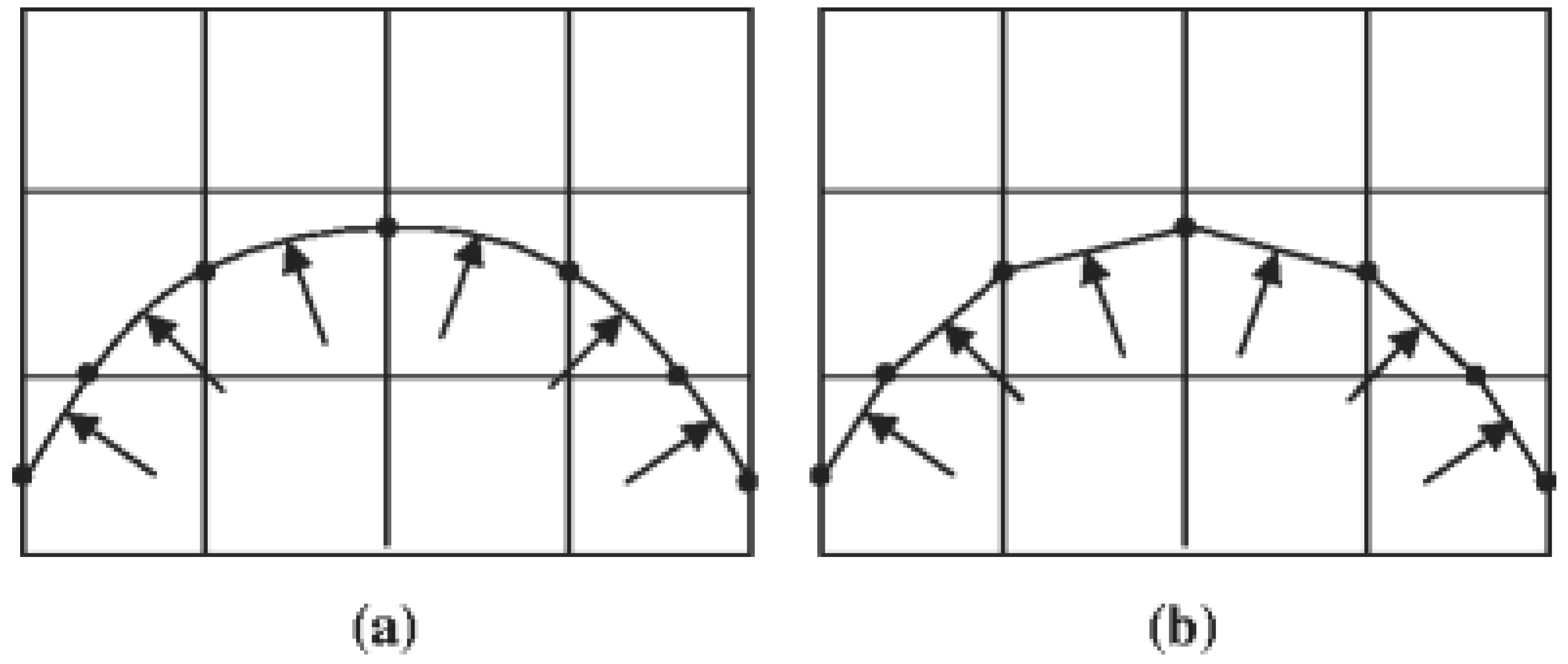
4.1. Identify the Boundary Using the DRLSE Method

In the DRLSE model, the boundary of the gray image is represented as the zero-level contour of the final level set function. The grayscale image (0–1) obtained in topology optimization is actually a 1-bit grayscale image. To use the DRLSE algorithm, the image must first be turned into an 8-bit grayscale image:
I = 255 − 255*x
where I is the 8-bit grayscale image data and x is the element node density matrix.
Since the boundary of the grayscale image is not obvious, the DRLSE algorithm does not necessarily find a suitable loading surface, which also makes it difficult to control the expansion of the loading surface during the optimization process. To overcome these types of problems, a density threshold is introduced, and the density of elements that is less than the density threshold is reset to zero during the image search. In this way, the obtained grayscale image has a clear boundary, and the expansion of the loading surface can also be controlled by adjusting the density threshold. The setting of the density threshold is similar to that in reference [19].

4.2. Design-Dependent Load Computing

In the process of finite element calculation, the load acting on the pressure-loading surface in the element must be transformed into the corresponding node. The pressure loading surface obtained with DRLSE is shown in Figure 1a. To simplify the calculation, in this research, the method recommended by Du and Olhoff [17] was adopted, and the line segment between the two intersections of the loaded surface and the element boundary was used as the new loading surface (Figure 1b). The process of converting the ballast into the nodal force in the pressure action element is shown in Figure 2, Figure 3 and Figure 4.
Assuming that the coordinates of the two intersection points of the pressure loading surface and the element boundary are ( x 1 , y 1 ) and ( x 2 , y 2 ) , the equivalent nodal load matrix f e acting on the element can be determined with the element shape function N and the load matrix . The integral over the action boundary is obtained [19]. Then, the following expression is obtained:
f e = L N T d l = P x 1 x 2 N T { Δ y Δ x 1 } d x
Converting the integral interval from [ x 1 , x 2 ] to [−1, 1], the above formula can be calculated using the Gaussian integral formula, and the following expression is obtained:
f e = L 2 1 1 N T d ξ { Δ y / L Δ x / L } = 1 2 i ω i N ( g i ) T { Δ y / L Δ x / L }
where P represents the magnitude of the pressure load, and ωi and gi are the i-th weight function and the corrected Gaussian quadrature point, respectively. Letting Δ x = x 1 x 2 , x ¯ = x 2 x 1 2 , and similarly for y , then:
g i = { 1 2 g i Δ x + x ¯ 1 2 g i Δ y + y ¯ }
After the above calculation, the pressure on the loading surface in the element is equivalent to the nodal load, and finite element analysis can then be carried out.

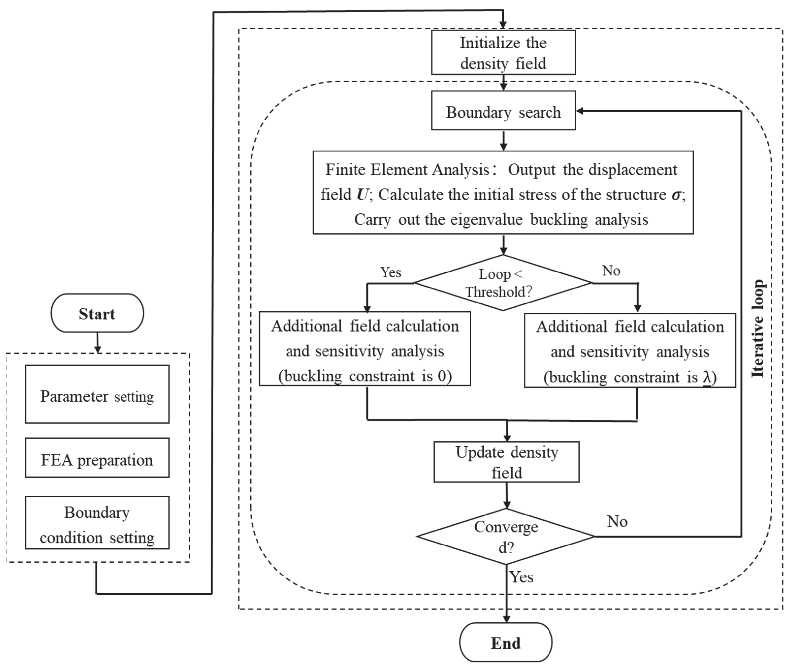
5. Optimization Algorithm

Based on the above finite element and sensitivity analyses, the topology optimization problem in Equation (1) can now be solved using a gradient-based optimization algorithm. In this research, the optimality criteria update optimization solver proposed by Ferrari et al. [13] and the parameters recommended by Ferrari et al. [13] were adopted. The flowchart of the proposed iterative solution algorithm is shown in Figure 5.
Step 1 Parameter setting: Define the number of finite elements in the design domain and the material properties, such as the Poisson’s ratio, elastic modulus, β, η, filter radius, volume constraints, and buckling constraints.
Step 2 Finite element preparation: Prepare the element stiffness matrix, node number of the geometric stiffness matrix, preparation matrix for density filtering, etc.
Step 3 Boundary condition setting: Set the boundary, load, and other conditions.
Step 4 Initialize the density field: Calculate the physical density by using linear density filters and projection filters.
Step 5 Boundary search: Based on the DRLSE loading surface search algorithm, search for the position where the force is applied and obtain the force vector.
Step 6 Finite element analysis: Perform finite element analysis.
Step 7 Sensitivity analysis: Calculate the sensitivities of the objective function, the K-S functions for the buckling constraints, and the material volume constraint.
Step 8 Update of the density field: Update the density field.
Step 9 Judgment of convergence condition: After judging whether the convergence condition is reached, the convergence automatically changes the buckling constraints to continue the optimization.
Step 10 Repeat or End: Repeat steps 4–10 and continue to iterate if not converged. Otherwise, end the loop and post-process the optimization results.

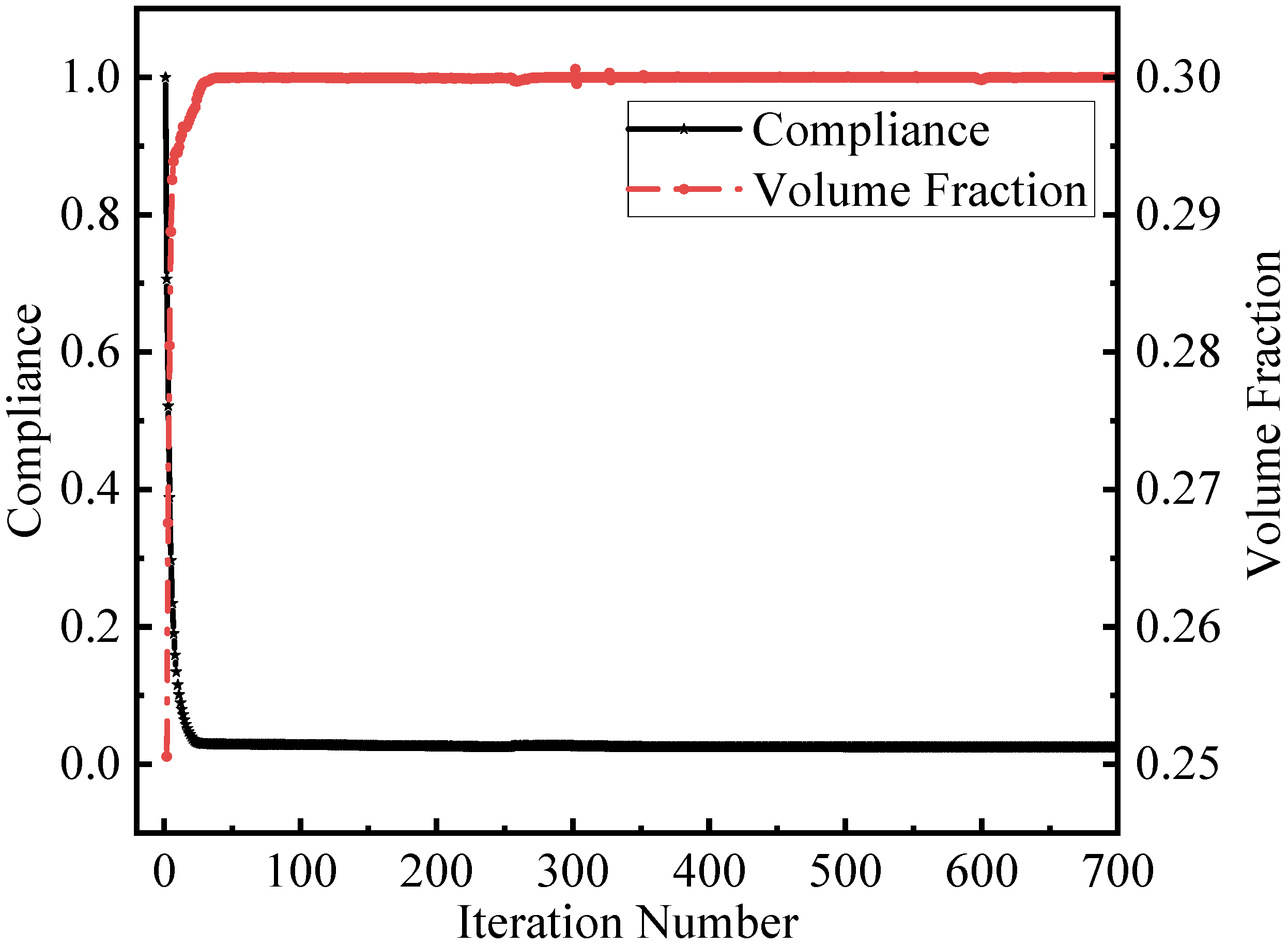
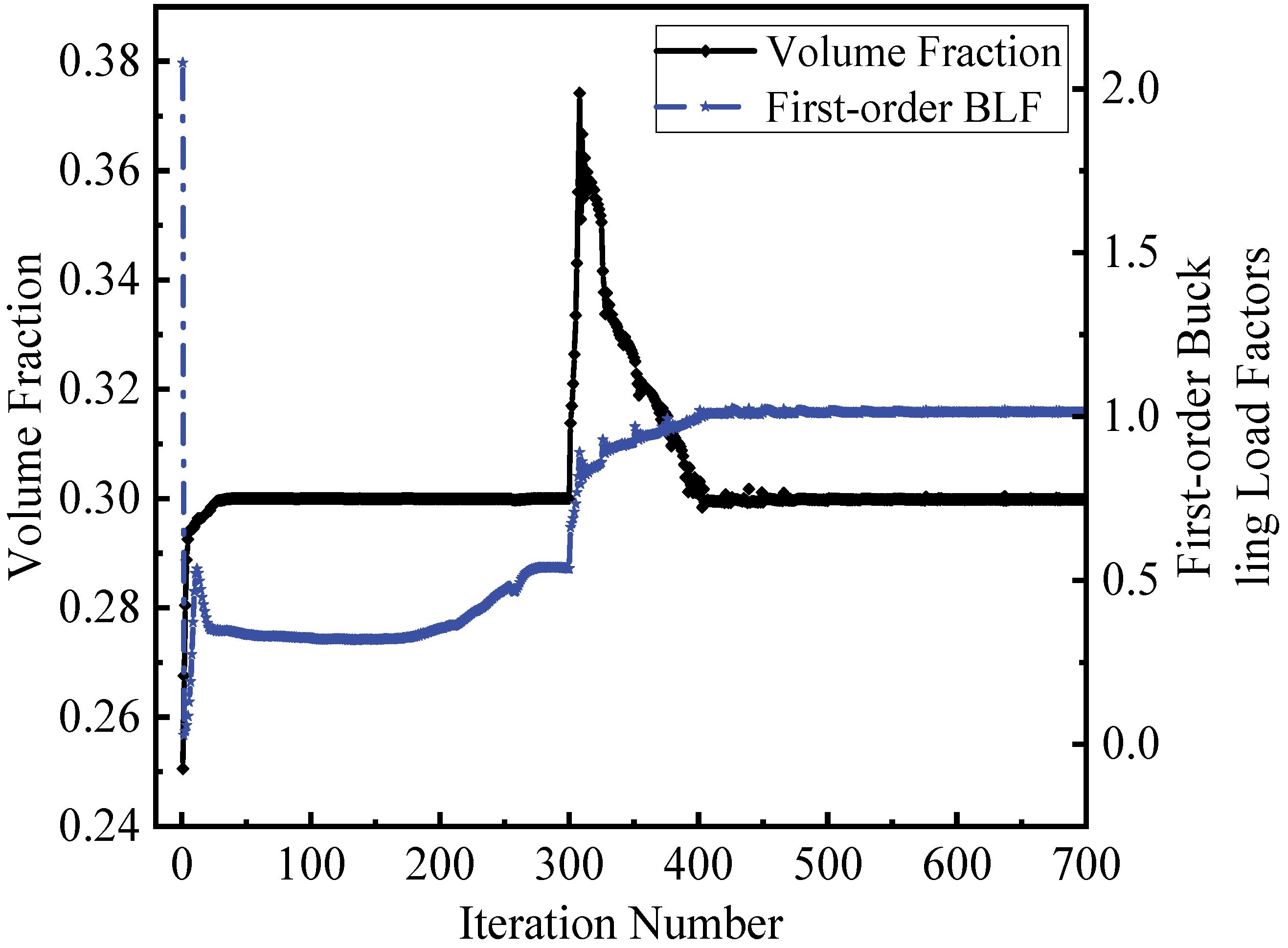
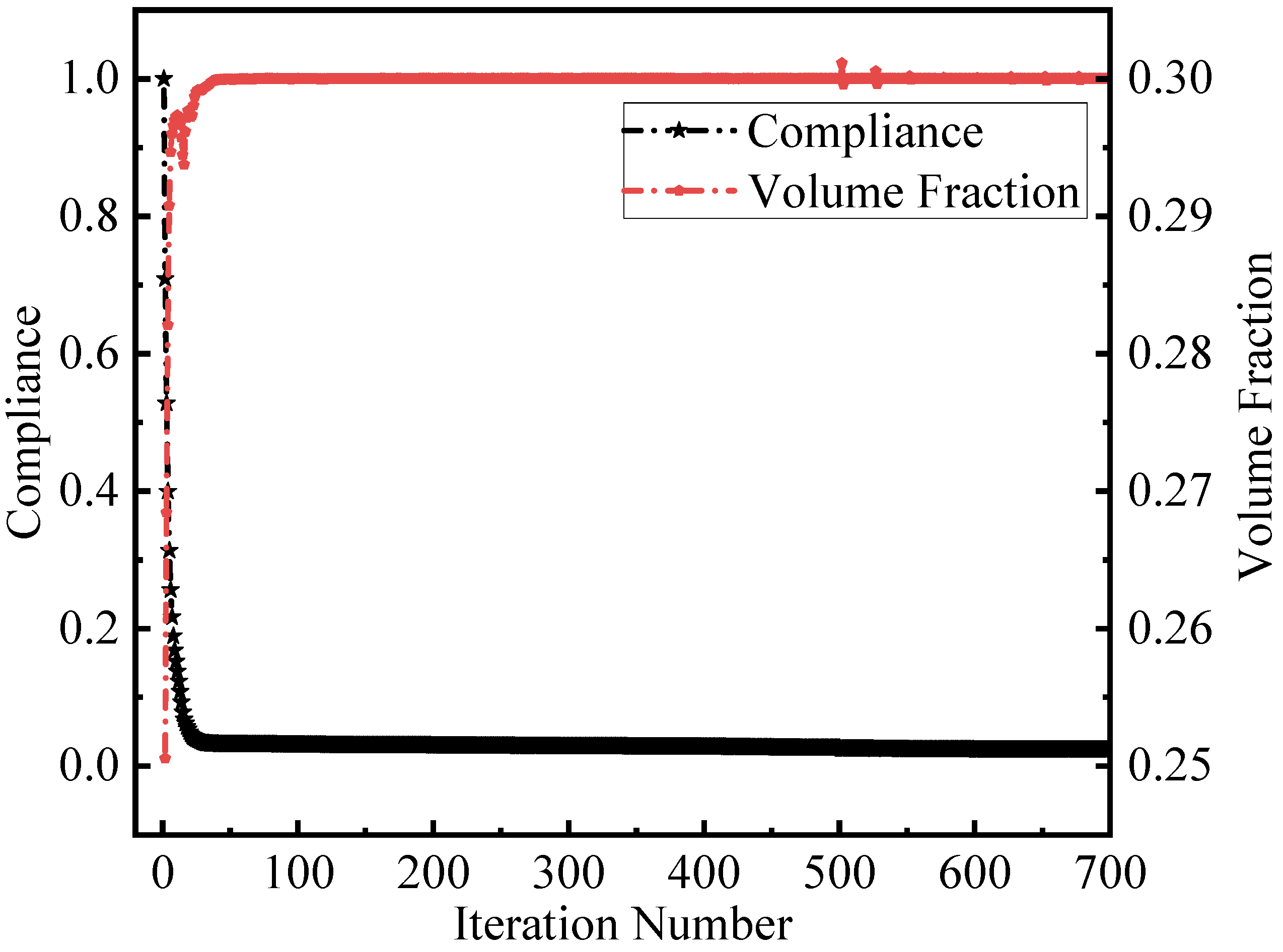
6. Numerical Examples

In this section, the effectiveness of the topology optimization model proposed in this paper is illustrated with numerical examples, such as arch structures subjected to external pressure. First, the initial solution was obtained with the compliance minimization model, which only considered volume constraints. Then, the buckling factor of the optimization result was used as a reference to determine the initial value of the buckling constraints when the topology optimization problem, with consideration of the buckling constraints, was performed. In the following numerical examples, Young’s modulus was set to 1, and Poisson’s ratio was set to 0.3. The optimization model was realized with MATLAB programming. The MATLAB version was R2020b. The eigs function in MATLAB was used to solve the structural eigenvalues and eigenvectors. The Lanczos algorithm was used to solve the symmetric matrix. The computer CPU used was an Intel(R) Xeon(R) E5-2678, the main frequency was 2.6 GHz, and the computer memory was 64 GB.

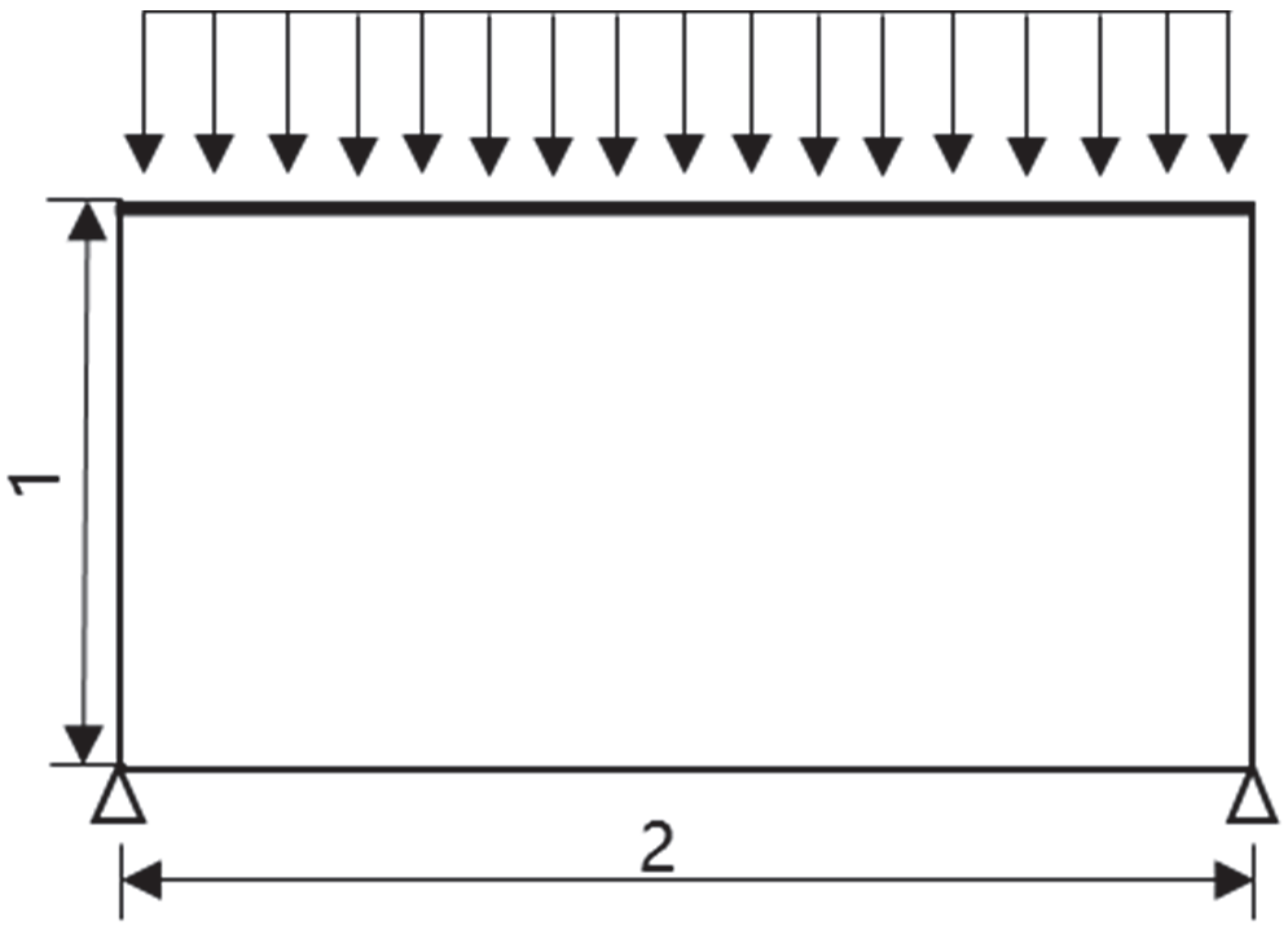
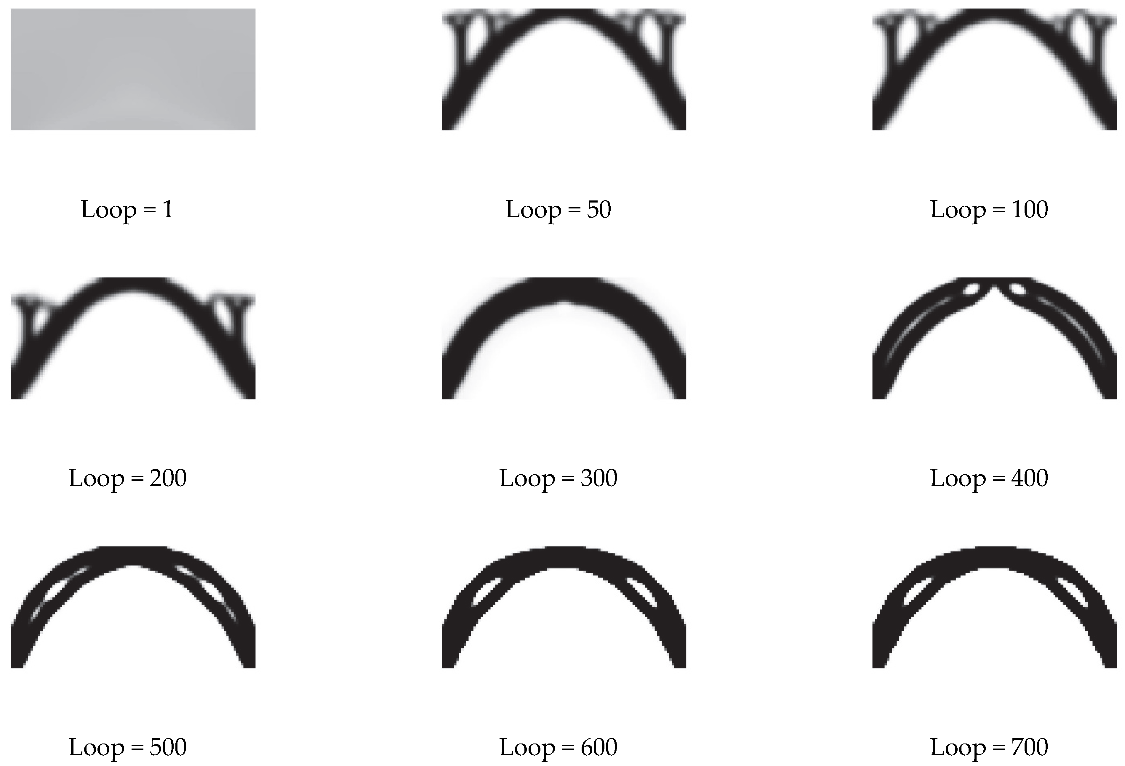
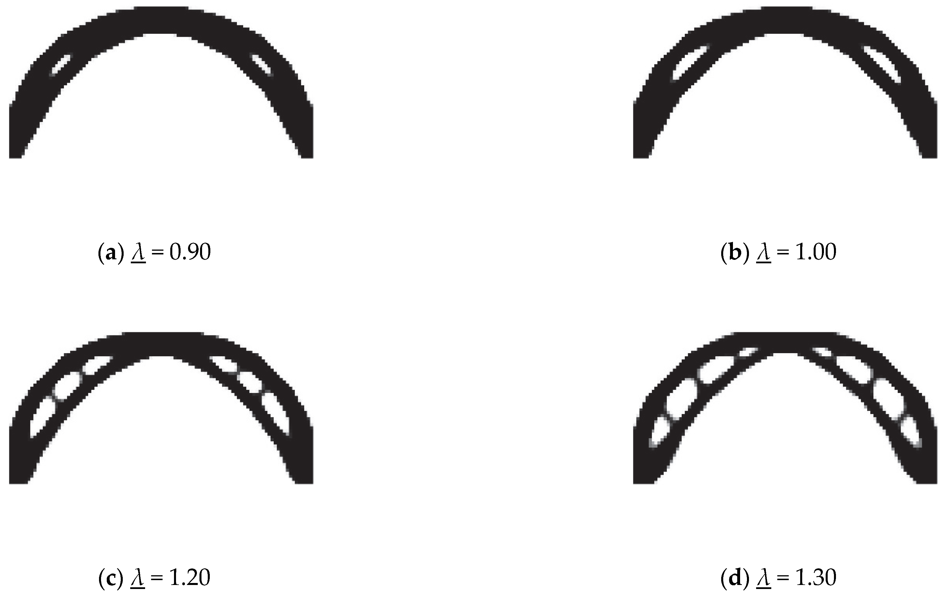
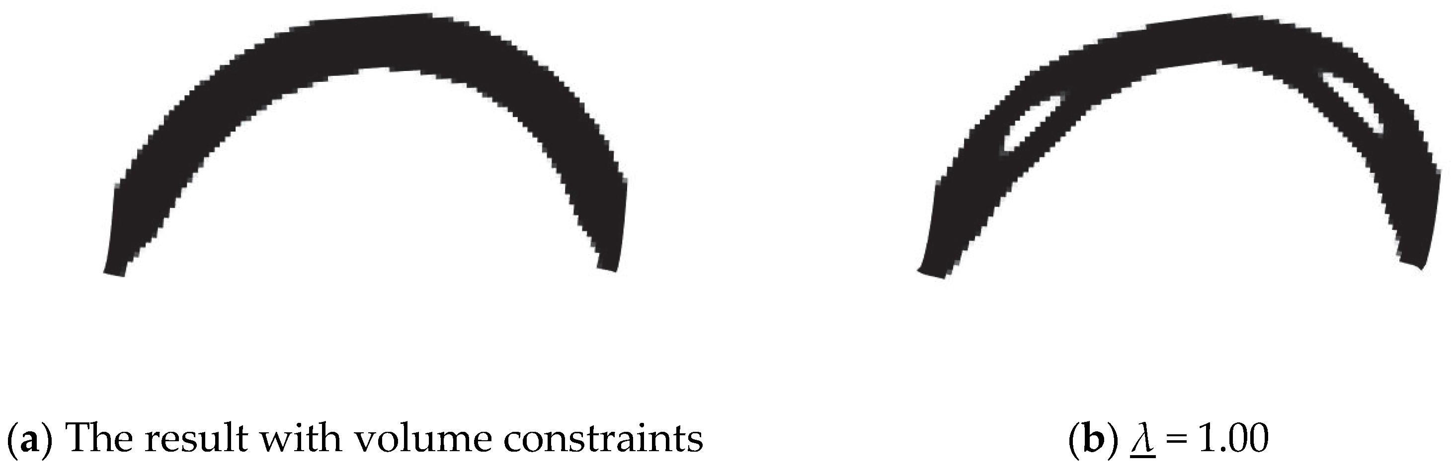
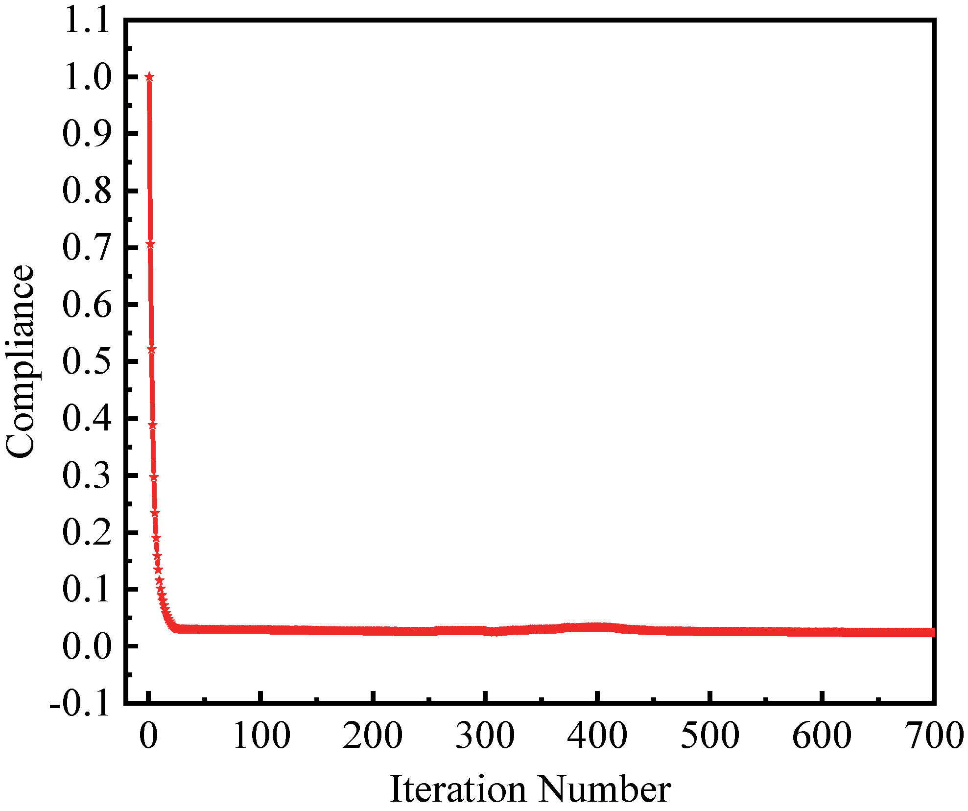
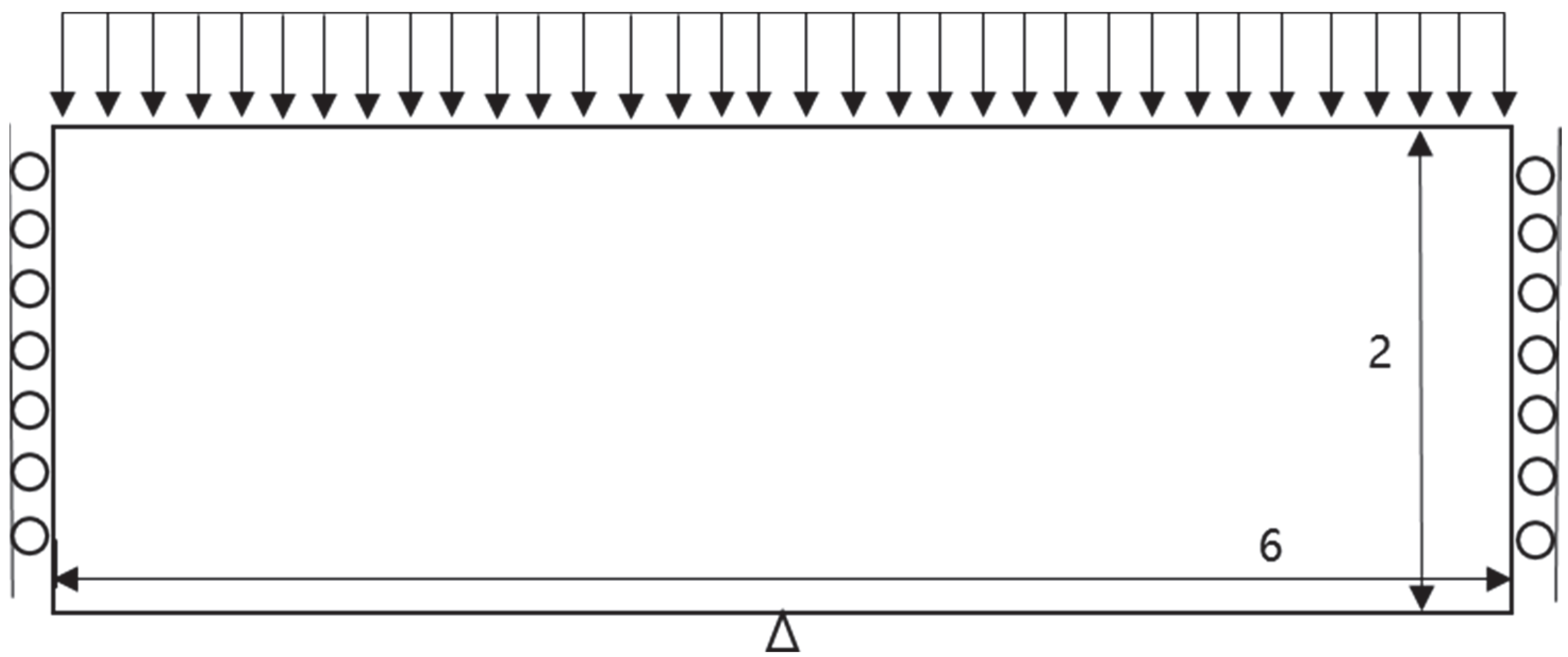
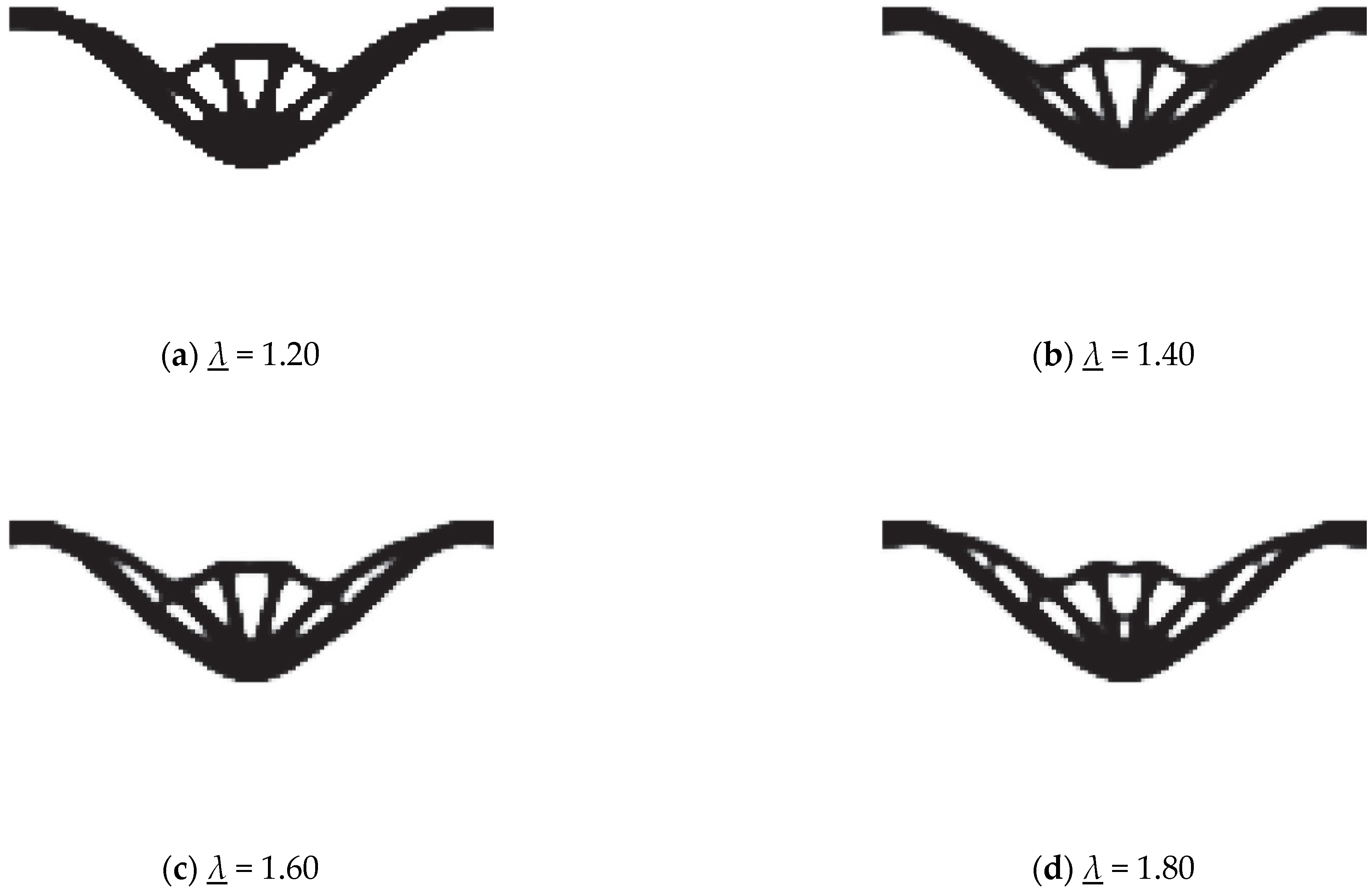
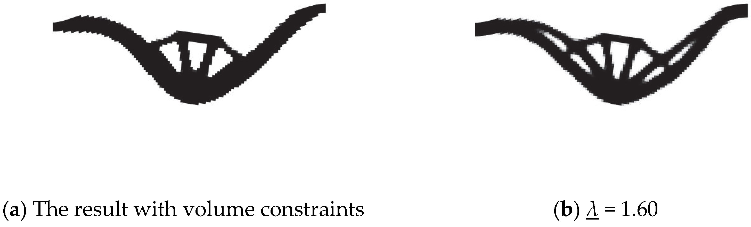
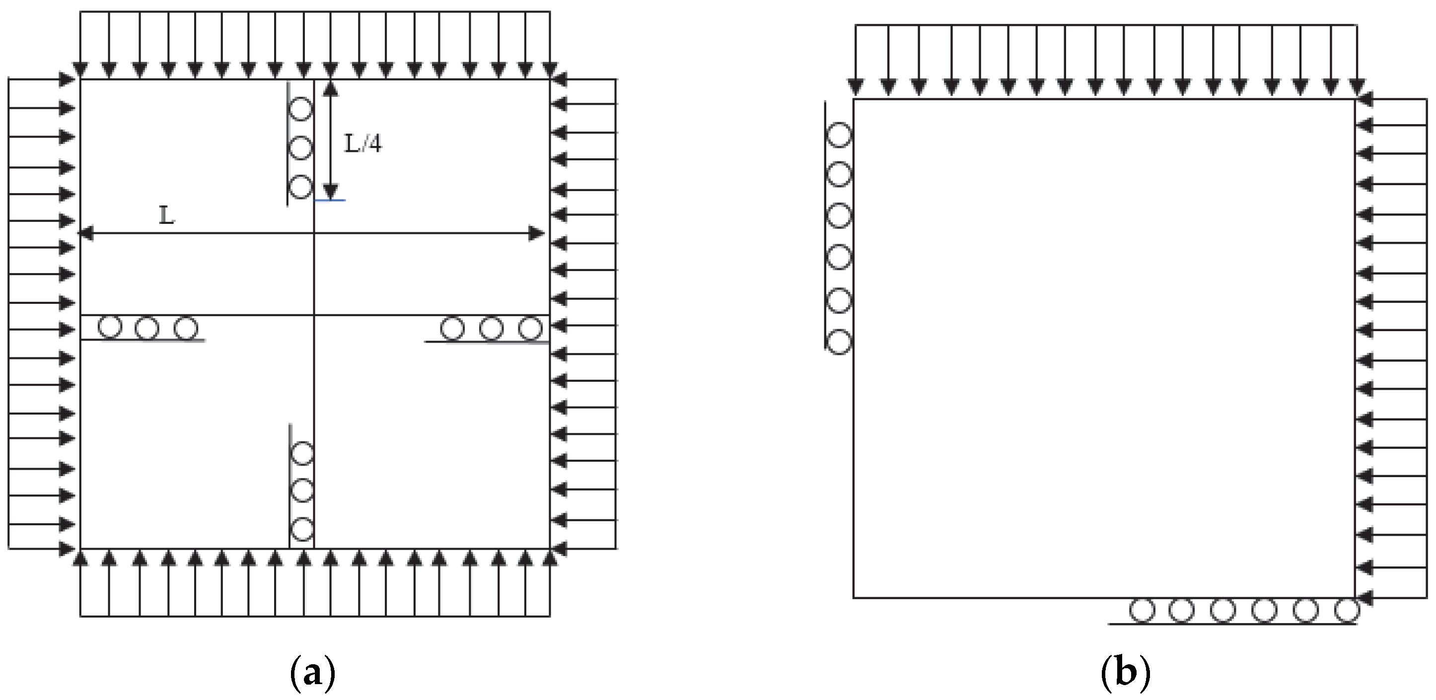
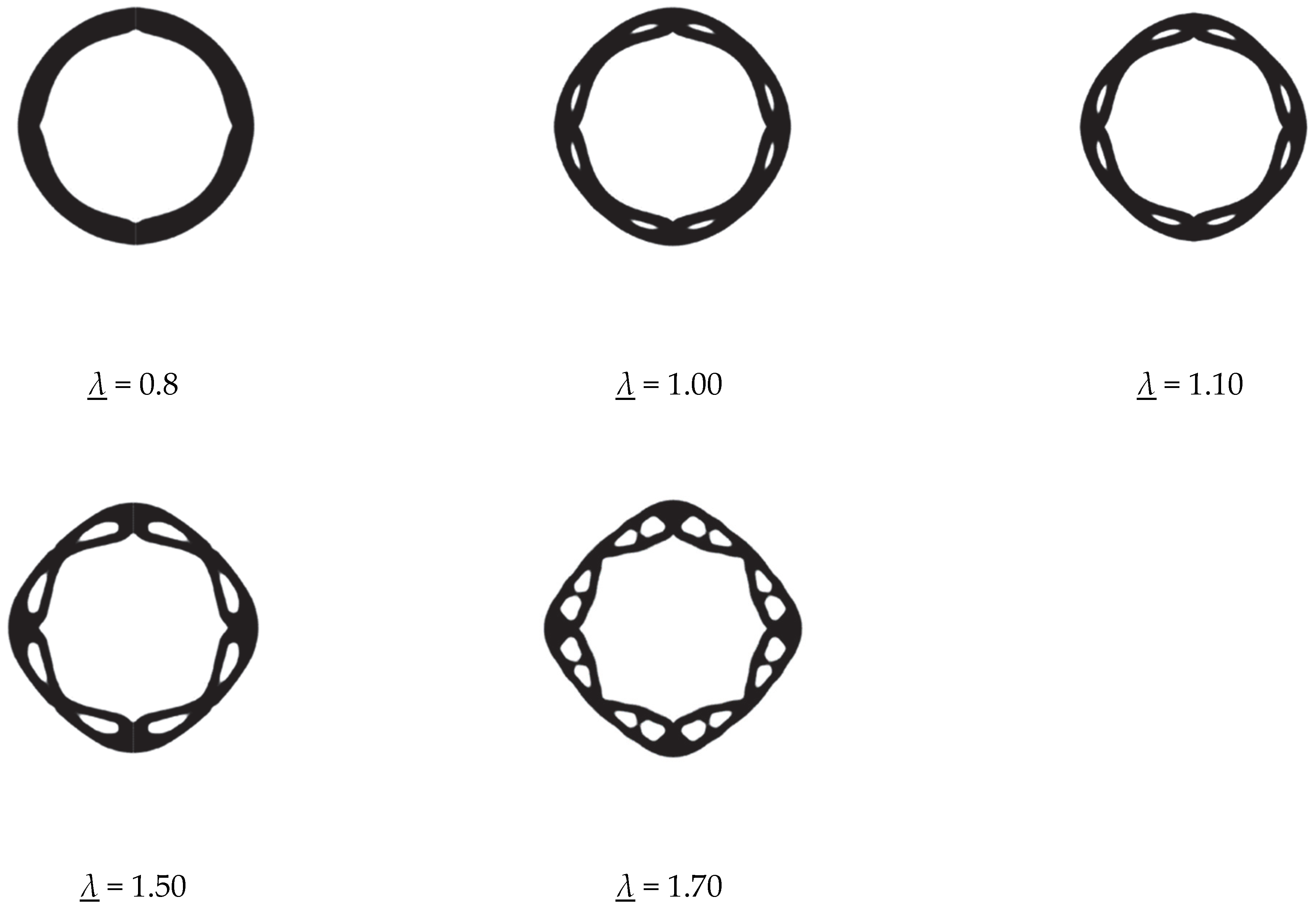
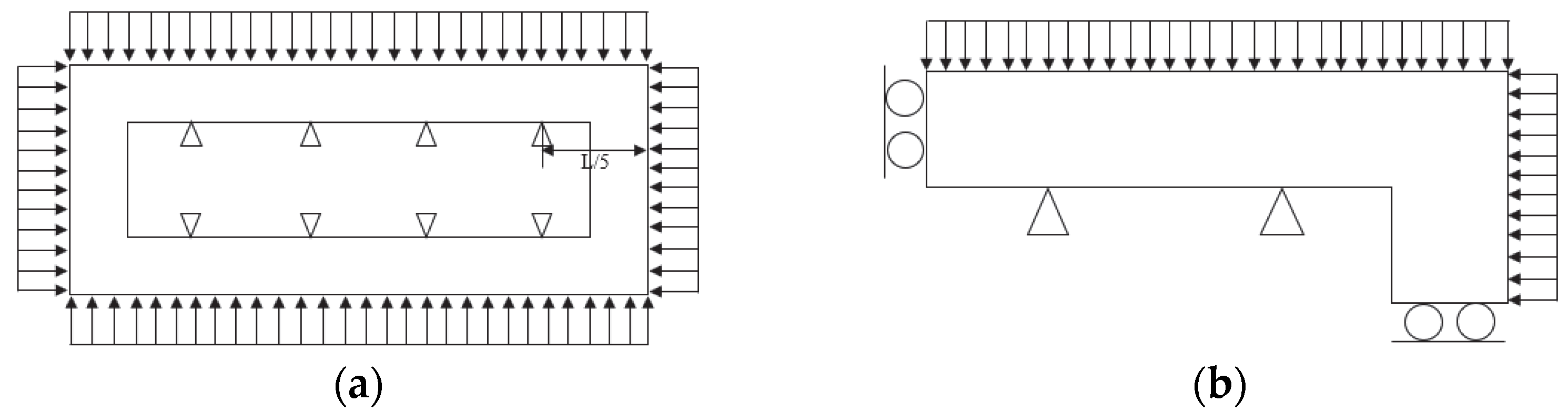
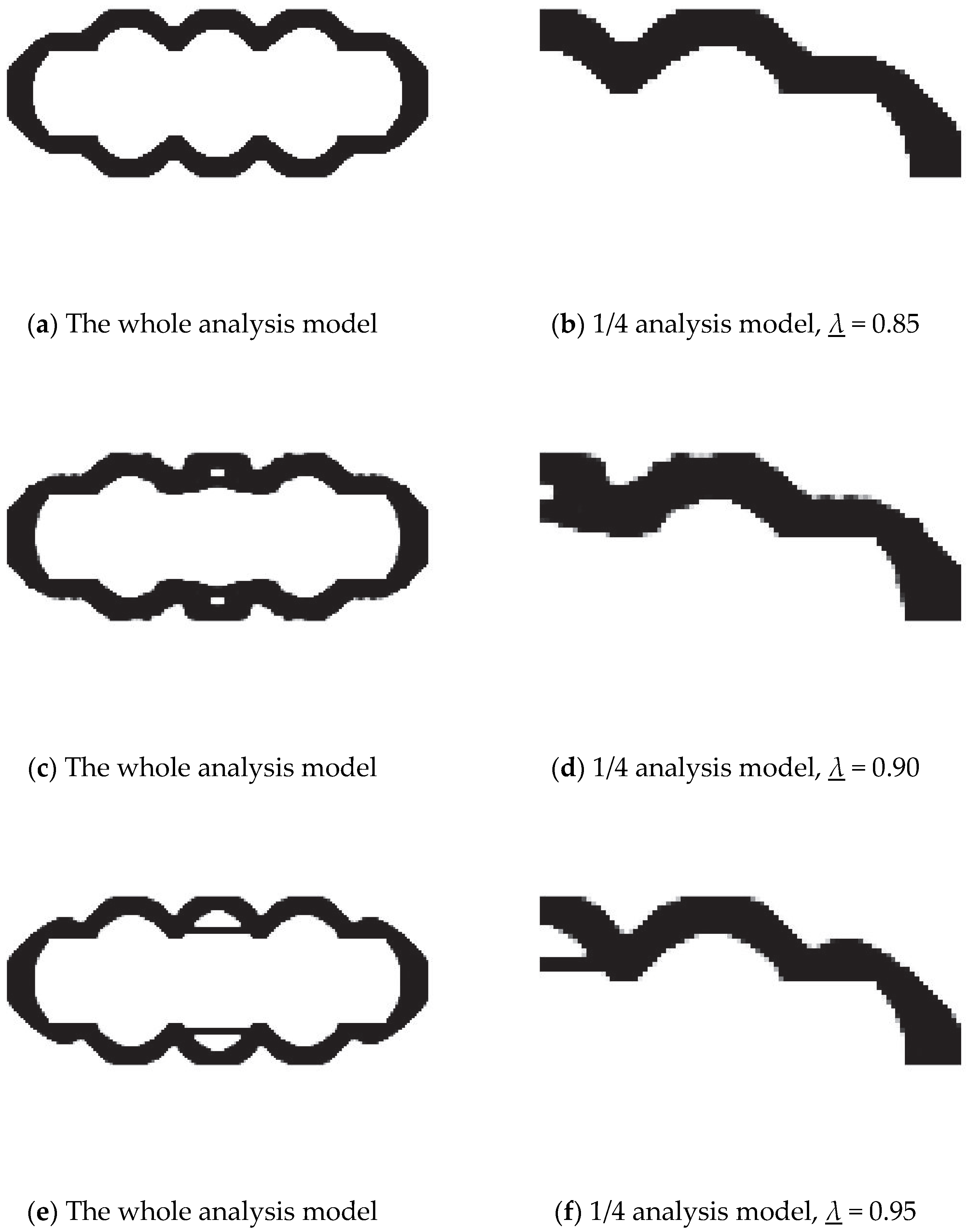
6.1. Arch Structure Subjected to External Pressure

First, a topology optimization design for the compliance minimization problem subjected to volume constraints was carried out. The final optimization result is shown in Figure 4. The area was divided into a 100 × 50 grid. The objective function value of the optimized structure was 2.44 × 10⁻², and the first-order buckling factor was 0.74. The corresponding convergence curve is shown in Figure 5.
Then, the topology optimization design subjected to buckling constraints was carried out, and the buckling constraints were taken as 0.9, 1.0, 1.2, and 1.3. The results are shown in Figure 6. The corresponding first-order buckling factors and compliance values were 0.91 and 2.30 × 10⁻², 1.01 and 2.35 × 10⁻², 1.21 and 2.58 × 10⁻², and 1.30 and 2.83 × 10⁻². In this numerical example, each iteration step lasted 0.8 s. To obtain the relationship between the first-order buckling factor and compliance, Table 1 was established.
Table 1 shows that when the volume fraction of the structural was constant, given the different buckling restraint values, the compliance of the structure increased with the increase of the buckling restraint value, which indicated that the improvement of the structural stability was at the expense of a small amount of structural stiffness. The above conclusion was the same as that in the literature 8. Figure 6 presents the intermediate topologies when the buckling constraint was 1.0. Figure 7 shows that when the buckling constraint was considered, the structure no longer maintained a complete arch structure, and the left and right supports expanded outward. When the buckling constraint was small, holes were generated inside. As the buckling constraint increased, the left and right supports on both sides changed into a porous structure, and there were more support rods to improve the stability of the structure, which was similar to Clausen et al. [10] using a porous filling structure to improve stability.
Figure 8 shows the optimization results for the compliance minimization subjected to the volume constraint and the first mode of the optimization results when the buckling constraint was 1.0. Since the low-order mode accounted for a large proportion of the response, and the low-order mode would be of more concern in engineering practice, only the first-order mode is given in this paper. Comparing the first-order modes of the two optimization results, it could be found that the stability was improved by expanding the left and right supports outward and adding holes when considering buckling constraints. Although the deformation region of the results considering buckling constraints was similar to the compliance minimization result, the buckling factor values were greatly increased, and the structure was more stable.
The final optimization results in this paper are consistent with the results of Mendes et al. [15], which are compared in Figure 9. Figure 10 and Figure 11 show the convergence history of the objective function, the structural volume fraction, and the first-order buckling factor when the buckling constraint was taken as 1.0. It can be seen from the convergence history that the proposed topology optimization model and the adopted optimization algorithm could stably converge when the topology optimization problem was solved with consideration of the stability constraints, which verified the feasibility of the model and algorithm.

6.2. Piston Design Subjected to Hydrostatic Pressure

A dam, also known as a piston structure, is a common structure under design-dependent loads. The initial design domain, initial pressure, and boundary conditions in this research are shown in Figure 12. The design area was a rectangular area of 6 m × 2 m. The structure was fixed in place at the midpoint of the bottom and horizontally fixed in place on the left and right sides. The value of the hydrostatic pressure was 6 × 10⁻³. The area was divided into a 120 × 40 grid. The design material volume fraction was 0.3 of the design area.
First, the topology optimization design of the compliance minimization problem subjected to volume constraints was examined. The final optimization result is shown in Figure 13. The objective function value of the optimized structure was 2.36 × 10⁻², and the first-order buckling factor was 0.84. The corresponding convergence curve is shown in Figure 14. In this numerical example, each iteration step lasted 1.8 s.
Then, the topology optimization design subjected to buckling constraints was examined. The results are shown in Figure 15. The corresponding first-order buckling factors and compliance values were 1.23 and 2.41 × 10⁻², 1.42 and 2.46 × 10⁻², 1.62 and 2.47 × 10⁻², and 1.82 and 2.53 × 10⁻², as shown in Table 2. From Table 2, one can obtain the same conclusion as that discussed in Section 6.1.
Figure 15 shows that the optimization results with consideration of the buckling constraint had a significant difference from the compliance minimization optimization results with consideration of the volume constraints. When the buckling constraint was 1.2, holes were generated at the left and right ends of the bottom, and the number of support rods increased. With the increase of the buckling constraint, the material at the rod connecting the bottom and the left and right ends expanded outward, the amount of base material decreased, the middle holes became wider, and the rods were slender. When the constraint value was increased to 1.6, new holes and small rod supports were generated. If it was further increased, more holes and small rods were generated on the left and right tie rods. This was the same as the change rule of the arched structure subjected to external pressure.
The final optimization results in this paper are consistent with the results of Mendes et al. [15], which are compared in Figure 16. Figure 17 shows the optimization results for compliance minimization subjected to the volume constraint and the first mode of optimization results when the buckling constraint was 1.6. Comparing the first-order modes of the two optimization results, we obtained the same conclusion as that discussed in Section 5.

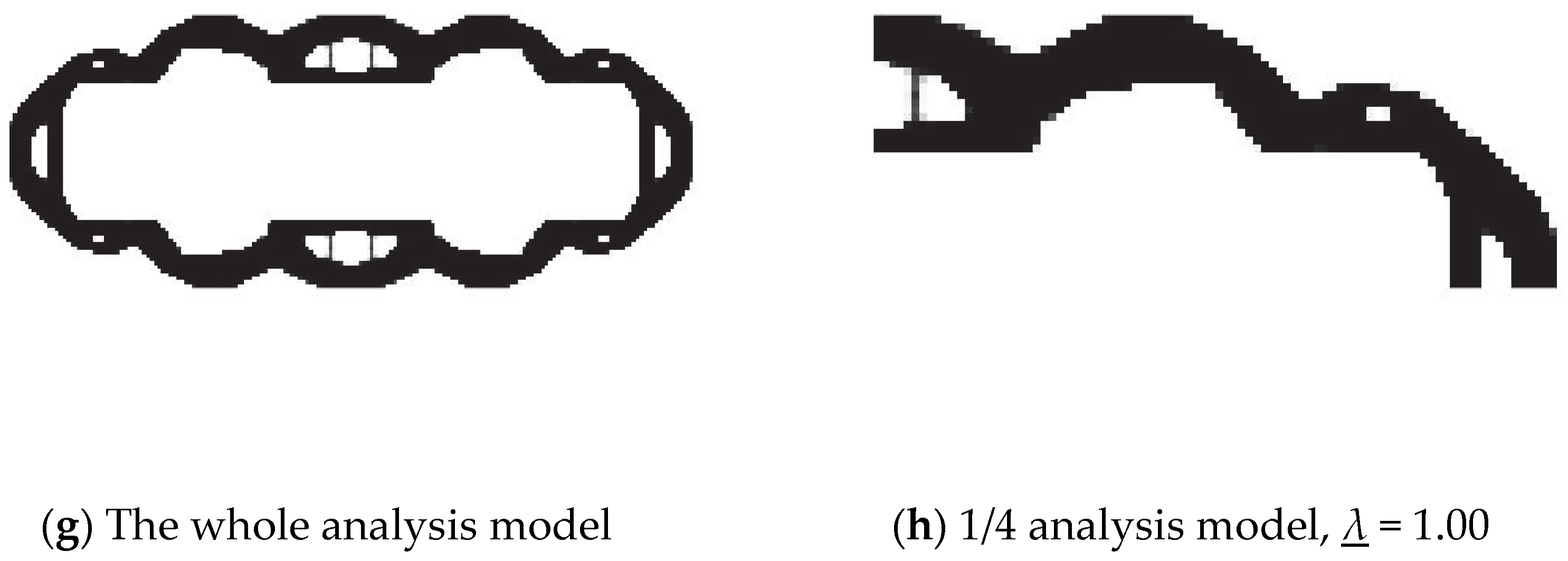
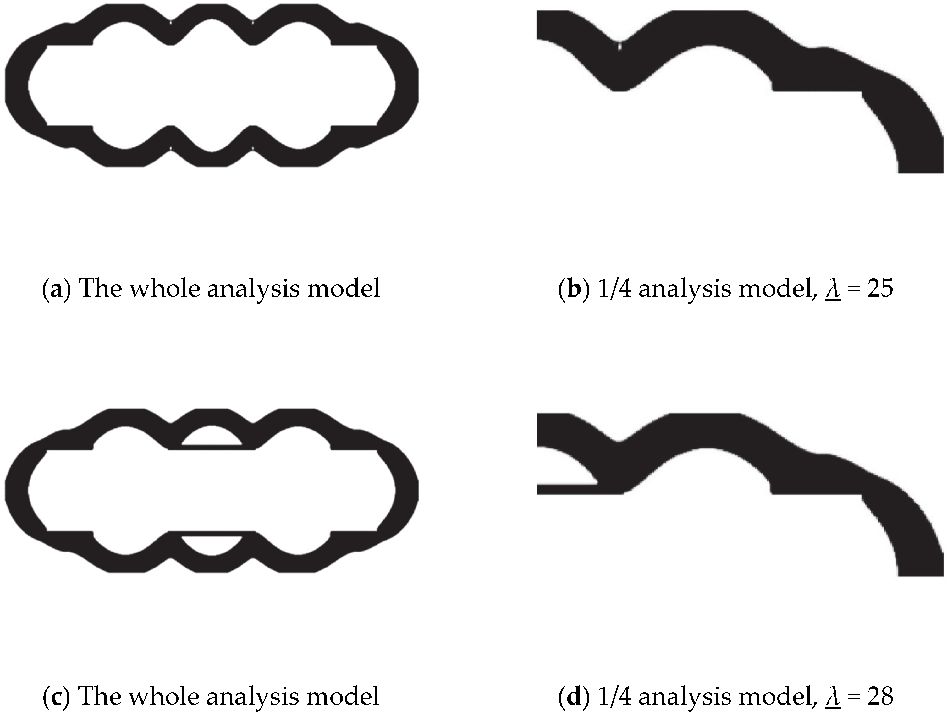
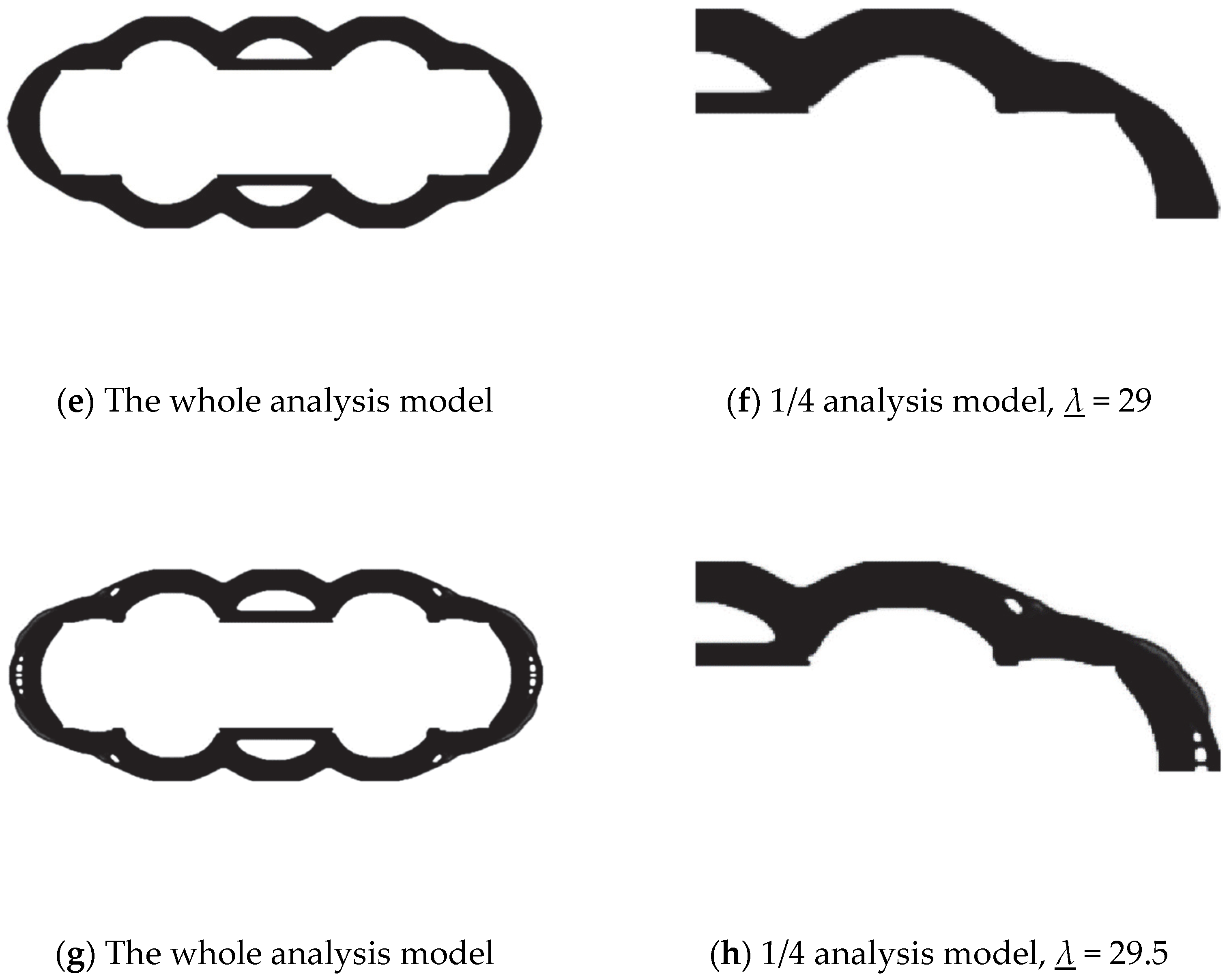
6.3. Structure Design Subjected to Hydrostatic Pressure

A ring-stiffened cylindrical hull is a commonly used pressure hull. Since the shape along the length of the cylinder is basically unchanged, in this research, a simplified plane strain model was adopted to study the optimal design of an underwater pressure hull. The initial design domain, initial pressure constraints, and boundary conditions are shown in Figure 18. To improve calculation efficiency, a 1/4 model was used for the calculation. The design area was a square area with dimensions of 1 m × 1 m. The value of the hydrostatic pressure was 6.5 × 10⁻³. The area was first divided into an 80 × 80 grid. The design material volume fraction was 0.1 of the design area.
First, a topology optimization design for the compliance minimization problem subjected to volume constraints was carried out. The final optimization result is shown in Figure 19. The first-order buckling factor of the optimized structure was 0.70. The optimization results subjected to different buckling constraints are shown in Figure 18.
Figure 20 shows that when the buckling constraints were considered, the result was significantly different from the structure for which compliance was minimized with only the volume constraints considered. When the buckling constraint was 0.80, the material moved toward the left and bottom constraints and toward the external expansion. When the buckling constraint increased to 1.7, a porous structure was formed on the left and right supports, and support rods were created to improve the stability of the structure. There were similarities in the arched structure subjected to external pressure.
The above final optimization structures were solved with 80 × 80 mesh grids, and the optimization results with large-scale mesh grids (300 × 300) subjected to different buckling constraints are shown in Figure 21. The results with the same buckling factor limit λ = 1.5 under different mesh resolutions were compared, and the four mesh grid divisions are 80 × 80, 200 × 200, 300 × 300, and 400 × 400, respectively. The optimization results are shown in Figure 22 and could prove the validity of the method under large-scale mesh grids.

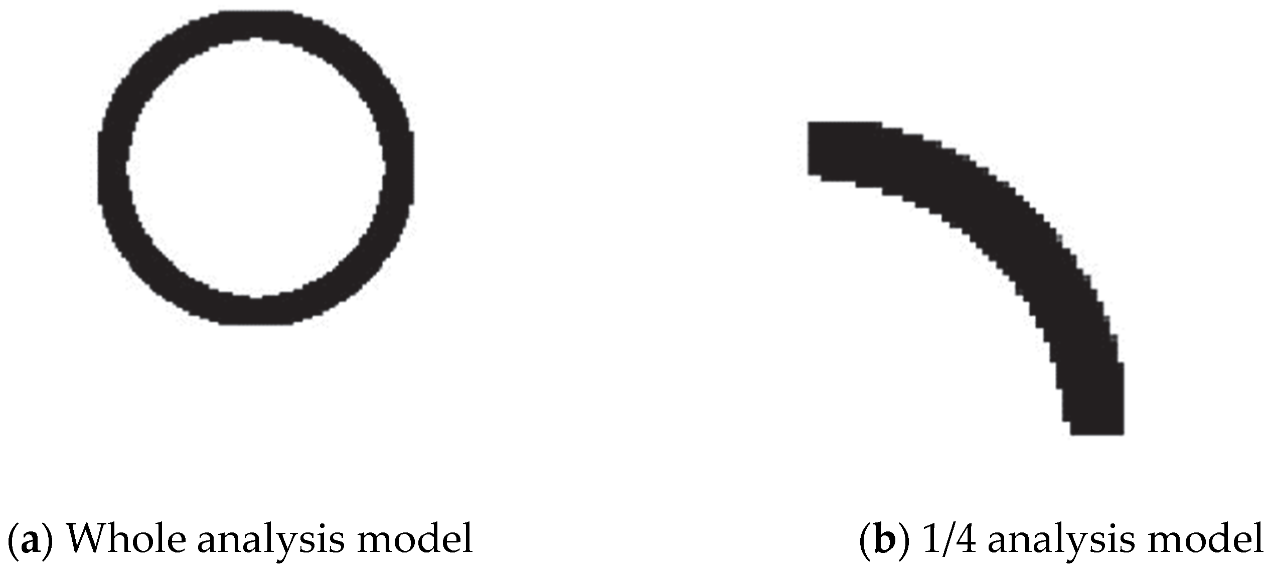
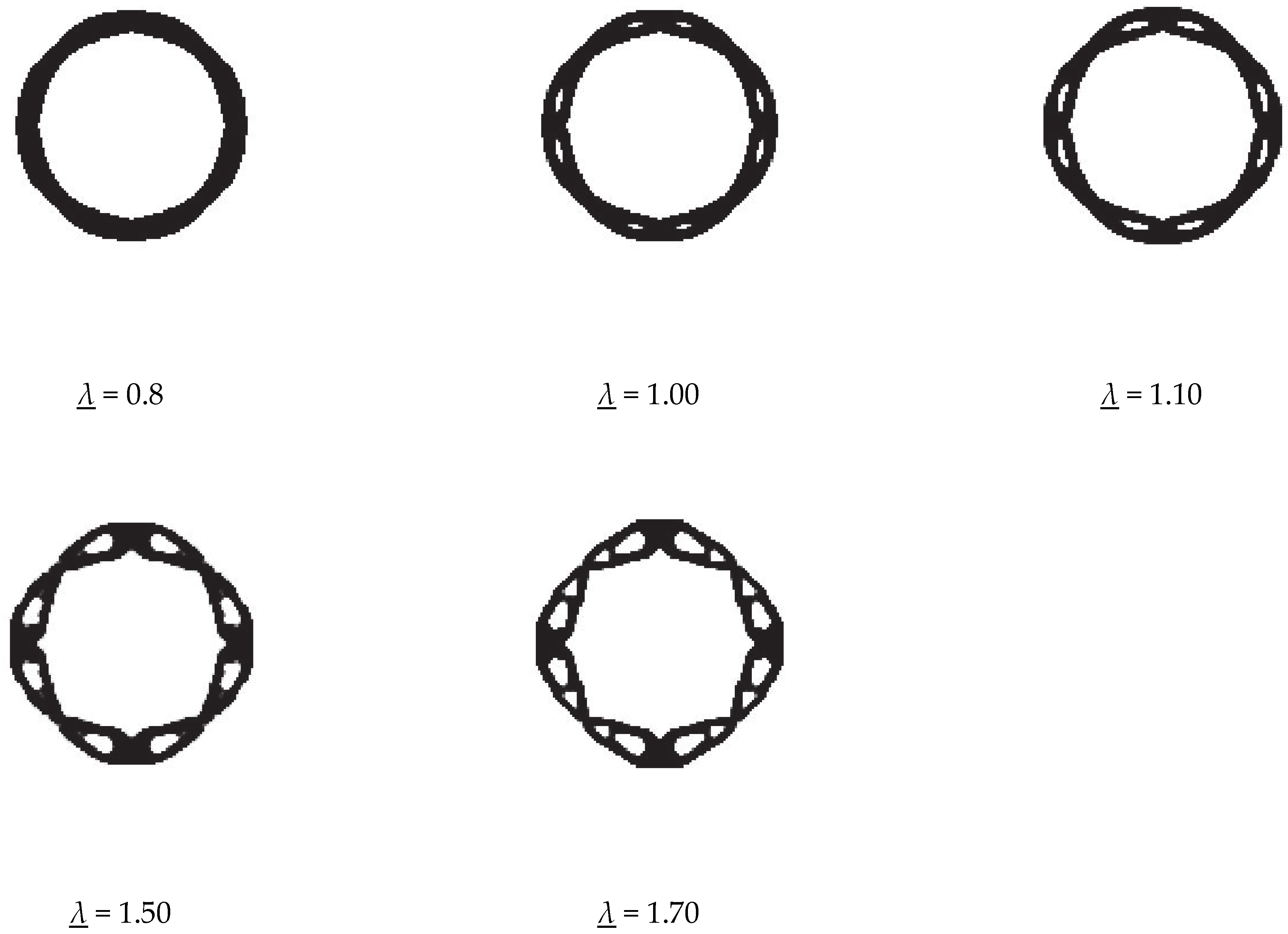
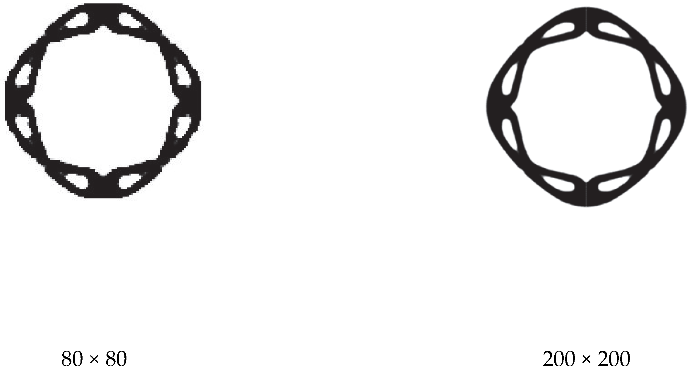
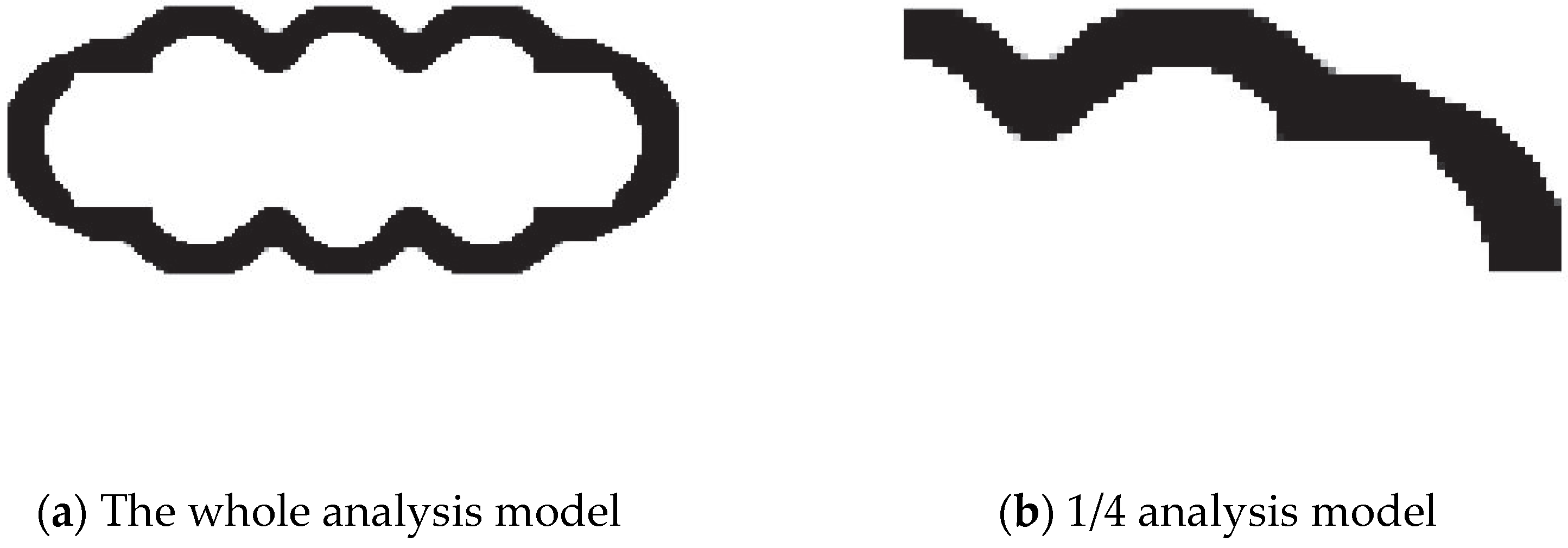
6.4. Multiple Intersecting Spherical Pressure Hulls

In practical applications, a pressure hull requires a certain intermediate blank area to be reserved for storing equipment and liquids [42]. Therefore, in this example, the optimal design of the axisymmetric model of the pressure hull was carried out. The initial design domain, initial pressure constraints, and boundary conditions are shown in Figure 23. To improve the calculation efficiency, the 1/4 model was used for the calculation. The design area was a rectangular area with dimensions of 2.5 m × 1 m. The value of the hydrostatic pressure was 2 × 10⁻². The area was divided into a 90 × 36 grid. The design material volume fraction was 0.3 of the design area.
First, the topology optimization design for the compliance minimization problem subjected to volume constraints was carried out. The final optimization result is shown in Figure 24. The first-order buckling factor of the optimized structure was 0.80. The optimization results subjected to different buckling constraints are shown in Figure 21.
The optimization results with different constraints are shown in Figure 25. When the buckling constraint was 0.85, the material moved to the constraint at the bottom. As the buckling constraint increased, the material gathered at the left constraint and generated holes or support rods. When the buckling constraint was increased to 1.00, two support rods were created, and a hole and a support rod were created at the bottom-right constraint, which was similar to the three previous examples.
The above final optimization structures were solved with 90 × 36 mesh grids, and the optimization results with large-scale mesh grids (270 × 108) subjected to different buckling constraints are shown in Figure 26. Because of the high concentrations of stress in the corners of the structures, with the increase in the scale of the mesh grid division, the stress in the corners increases. This results in an increase in the value of the determinant of the geometric stiffness matrix, so the values of the buckling factor become smaller. For a certain pressure structure, the critical buckling loads were constant and equal to the buckling factor, timing the hydrostatic pressure. Therefore, to highlight the clear change in the structures with increasing buckling factor values, hydrostatic pressure was set to 2 × 10⁻⁴ in this numerical example, and the buckling factor was set to 25–29.5.

7. Conclusions

In this paper, an algorithm for topology optimization for minimum compliance with material volume and buckling constraints under design-dependent loads was developed. The structural topology optimization problems were solved using the SIMP method along with a pressure boundary searching scheme based on the DRLSE model to deal with design-dependent loads. The K-S aggregation function was used to reduce multiple constraints to a single constraint and replace the original buckling constraints, which not only improved the smoothness of the original buckling constraints and caused the solution to converge to a certain extent but also reduced the number of constraints.
The numerical examples demonstrated the effectiveness and reliability of the algorithm. The results of the arch structure and piston examples showed that the compliance minimization problems subject to buckling and volume constraints and the compliance minimization problems subject to volume constraints could result in considerably different topologies. The compliance minimization subject to buckling and volume constraints generally resulted in a more fully stable design when compared to the compliance minimization with the same volume constraints for which buckling constraints were not considered. In engineering structure design, stability is a critical factor that cannot be ignored. Hence, the buckling constrained approach is of importance in topology optimization.
The application of the algorithm in practical engineering design is the design of underwater structures, and the optimal results with different buckling factor limits are shown in this work. The results showed that more sandwich support structures were produced with increasing buckling factor limits. In addition, the method could be used for designing multiple intersecting spherical pressure hulls that have complex boundary conditions. Therefore, the developed algorithm has better applicability.
The future direction of this research is to simultaneously consider more design constraints, such as stress constraints and buoyancy constraints. In addition, the topology optimization problem will be extended into three dimensions in future work.

Author Contributions

Conceptualization, M.Z.; methodology, K.Z.; software, K.Z.; validation, Y.J.; formal analysis, Y.J.; writing—original draft preparation, K.Z.; writing—review and editing, Y.J. and J.X.; supervision, M.Z. All authors have read and agreed to the published version of the manuscript.

Funding

The authors would like to deeply thank the National Natural Sciences Foundation of China (U2067220, 51779139), the Young Talent Project of China National Nuclear Corporation, and the Top Young Talents of Ten Thousand Talents Plan for support.

Institutional Review Board Statement

The article does not contain any studies with human participants or animals performed by any of the authors.

Informed Consent Statement

Not applicable.

Data Availability Statement

The authors state that all the data necessary to replicate the results are presented in the manuscript. Relevant parts of the code can be shared upon contacting the corresponding author.

Acknowledgments

The authors thank Sigmund for providing the 250-line MATLAB source code for considering buckling constraint topology optimization based on the SIMP method.

Conflicts of Interest

On behalf of all authors, the corresponding author states that there are no conflict of interest.

References

  1. Hoang, V.N.; Wang, X.; Xuan, H.N. A three-dimensional multiscale approach to optimal design of porous structures using adaptive geometric components. Compos. Struct. 2021, 273, 114296. [Google Scholar] [CrossRef]
  2. Hoang, V.N.; Nguyen, H.B.; Xuan, H.N. Explicit topology optimization of nearly incompressible materials using polytopal composite elements. Adv. Eng. Softw. 2020, 149, 102903. [Google Scholar] [CrossRef]
  3. Hoang, V.N.; Nguyen, N.L.; Tran, D.Q.; Vu, Q.V.; Xuan, H.N. Data-driven geometry-based topology optimization. Struct. Multidiscip. Optim. 2022, 65, 69. [Google Scholar] [CrossRef]
  4. Neves, M.M.; Rodrigues, H.; Guedes, J.M. Generalized topology design of structures with a buckling load criterion. Struct. Optim. 1995, 10, 71–78. [Google Scholar] [CrossRef]
  5. Neves, M.M.; Sigmund, O.; Bendsøe, M.P. Topology optimization of periodic microstructures with a penalization of highly localized buckling modes. Int. J. Numer. Methods Eng. 2002, 54, 809–834. [Google Scholar] [CrossRef]
  6. Zhou, M. Topology optimization for shell structures with linear buckling responses. In Proceedings of the WCCM VI in conjunction with APCOM’04, Beijing, China, 5–10 September 2004; pp. 795–800. [Google Scholar]
  7. Wang, W.; Ye, H.; Sui, Y. Lightweight Topology Optimization with Buckling and Frequency Constraints Using the Independent Continuous Mapping Method. Acta Mech. Solida Sin. 2019, 32, 310–325. [Google Scholar] [CrossRef]
  8. Gao, X.J.; Ma, H.T. Topology optimization of continuum structures under buckling constraints. Comput. Struct. 2015, 157, 142–152. [Google Scholar] [CrossRef]
  9. Gao, X.J.; Ma, H.T.; Chen, G.F. Improving the overall performance of continuum structures: A topology optimization model considering stiffness, strength and stability. Comput. Methods Appl. Mech. Engrg. 2020, 359, 112660. [Google Scholar] [CrossRef]
  10. Clausen, A.; Aage, N.; Sigmund, O. Exploiting additive manufacturing infill in topology optimization for improved buckling load. Engineering 2016, 2, 250–257. [Google Scholar] [CrossRef] [Green Version]
  11. Ferrari, F.; Sigmund, O. Revisiting topology optimization with buckling constraints. Struct. Multidiscip. Optim. 2019, 59, 1401–1415. [Google Scholar] [CrossRef]
  12. Ferrari, F.; Sigmund, O. Towards solving large-scale topology optimization problems with buckling constraints at the cost of linear analyses. Comput. Methods Appl. Mech. Engrg. 2020, 363, 112911. [Google Scholar] [CrossRef] [Green Version]
  13. Ferrari, F.; Sigmund, O.; Guest, J.K. Topology optimization with linearized buckling criteria in 250 lines of MATLAB. Struct. Multidiscip. Optim. 2021, 63, 3045–3066. [Google Scholar] [CrossRef]
  14. Zhang, W.; Jiu, L.; Meng, L. Buckling-constrained topology optimization using feature-driven optimization method. Struct. Multidiscip. Optim. 2022, 65, 37. [Google Scholar] [CrossRef]
  15. Mendes, E.; Sivapuram, R.; Rodriguez, R.; Sampaio, M.; Picelli, R. Topology optimization for stability problems of submerged structures using the TOBS method. Comput. Struct. 2022, 259, 106685. [Google Scholar] [CrossRef]
  16. Hammer, V.B.; Olhoff, N. Topology optimization of continuum structures subjected to pressure loading. Struct. Multidiscip. Optim. 2000, 19, 85–92. [Google Scholar] [CrossRef]
  17. Du, J.; Olhoff, N. Topological optimization of continuum structures with design-dependent surface loading—Part II: Algorithm and examples for 3D problems. Struct. Multidiscip. Optim. 2004, 27, 166–177. [Google Scholar] [CrossRef]
  18. Zhang, H.; Zhang, X.; Liu, S.T. A new boundary search scheme for topology optimization of continuum structures with design-dependent loads. Struct. Multidiscip. Optim. 2008, 37, 121–129. [Google Scholar] [CrossRef]
  19. Lee, E.; Martins, J.R.R.A. Structural topology optimization with design-dependent pressure loads. Comput. Methods Appl. Mech. Engrg. 2012, 233, 40–48. [Google Scholar] [CrossRef]
  20. Acar, O.; Saglam, H.; Saka, Z. Measuring curvature of trajectory traced by coupler of an optimal four-link spherical mechanism. Measurement 2021, 176, 109189. [Google Scholar] [CrossRef]
  21. Kuntoglu, M.; Acar, O.; Gupta, M.K.; Saglam, H.; Sarikaya, M.; Giasin, K.; Pimenov, D.Y. Parametric optimization for cutting forces and material removal rate in the turning of AISI 5140. Machines 2021, 9, 90. [Google Scholar] [CrossRef]
  22. Wang, C.F.; Zhao, M.; Ge, T. Structural topology optimization with design-dependent pressure loads. Struct. Multidiscip. Optim. 2016, 53, 1005–1018. [Google Scholar] [CrossRef]
  23. Li, C.; Xu, C.; Gui, C.; Fox, M.D. Distance Regularized Level Set Evolution and Its Application to Image Segmentation. IEEE Trans. Image Process. 2010, 19, 3243–3254. [Google Scholar] [CrossRef] [PubMed]
  24. Li, Z.-M.; Yu, J.; Yu, Y.; Xu, L. Topology optimization of pressure structures based on regional contour tracking technology. Struct. Multidiscip. Optim. 2018, 58, 687–700. [Google Scholar] [CrossRef]
  25. Chen, B.C.; Kikuchi, N. Topology optimization with design-dependent loads. Finite Elem. Anal. Des. 2001, 37, 57–70. [Google Scholar] [CrossRef]
  26. Bourdin, B.; Chambolle, A. Design-dependent loads in topology optimization. ESAIM-Control. Optim. Calc. Var. 2003, 9, 19–48. [Google Scholar] [CrossRef]
  27. Sigmund, O.; Clausen, P.M. Topology optimization using a mixed formulation: An alternative way to solve pressure load problems. Comput. Methods Appl. Mech. Engrg. 2007, 196, 1874–1889. [Google Scholar] [CrossRef] [Green Version]
  28. Picelli, R.; Vicente, W.M.; Pavanello, R. Bi-directional evolutionary structural optimization for design-dependent fluid pressure loading problems. Engrg. Optim. 2014, 47, 1–19. [Google Scholar] [CrossRef]
  29. Picelli, R.; Vicente, W.M.; Pavanello, R. Evolutionary topology optimization for structural compliance minimization considering design-dependent FSI loads. Finite Elem. Anal. Des. 2017, 135, 44–55. [Google Scholar] [CrossRef]
  30. Sivapuram, R.; Picelli, R. Topology optimization of binary structures using integer linear programming. Finite Elem. Anal. Des. 2018, 139, 49–61. [Google Scholar] [CrossRef]
  31. Guo, X.; Zhao, K.; Gu, Y.X. Topology optimization with design-dependent loads by level set approach. In Proceedings of the 10th AIAA/ISSMO Multidisciplinary Analysis and Optimization Conference, Albany, NY, USA, 30 August–1 September 2004. [Google Scholar]
  32. Jiang, Y.T.; Zhao, M. Topology optimization under design-dependent loads with the parameterized level-set method based on radial-basis functions. Comput. Methods Appl. Mech. Engrg. 2020, 369, 113255. [Google Scholar] [CrossRef]
  33. Xia, Q.; Wang, M.Y.; Shi, T.L. Topology optimization with pressure load through a level set method. Comput. Methods Appl. Mech. Engrg. 2015, 283, 177–195. [Google Scholar] [CrossRef]
  34. Emmendoerfer, H.; Fancello, E.A.; Silva, E.C.N. Level set topology optimization for design-dependent pressure load problems. Int. J. Numer. Methods Eng. 2018, 115, 825–848. [Google Scholar] [CrossRef]
  35. Picelli, R.; Neofytou, A.; Kim, H.A. Topology optimization for design-dependent hydrostatic pressure loading via the level-set method. Struct. Multidiscip. Optim. 2019, 60, 1313–1326. [Google Scholar] [CrossRef] [Green Version]
  36. Kumar, P.; Frouws, J.S.; Langelaar, M. Topology optimization of fluidic pressure-loaded structures and compliant mechanisms using the Darcy method. Struct. Multidiscip. Optim. 2020, 61, 1637–1655. [Google Scholar] [CrossRef] [Green Version]
  37. Ibhadode, O.; Zhang, Z.; Rahnama, P.; Bonakdar, A.; Toyserkani, E. Topology optimization of structures under design-dependent pressure loads by a boundary identification-load evolution (BILE) model. Struct. Multidiscip. Optim. 2020, 62, 1865–1883. [Google Scholar] [CrossRef]
  38. Wang, C.F.; Qian, X.P. A density gradient approach to topology optimization under design-dependent boundary loading. J. Comput. Phys. 2020, 411, 109398. [Google Scholar] [CrossRef]
  39. Bourdin, B. Filters in topology optimization. Int. J. Numer. Methods Eng. 2001, 50, 2143–2158. [Google Scholar] [CrossRef]
  40. Wang, F.W.; Lazarov, B.S.; Sigmund, O. On projection methods, convergence and robust formulations in topology optimization. Struct. Multidiscip. Optim. 2010, 43, 767–784. [Google Scholar] [CrossRef]
  41. Rodrigues, H.C.; Guedes, J.M.; Bendsøe, M.P. Necessary conditions for optimal design of structures with a non-smooth eigenvalue based criterion. Struct. Optim. 1995, 9, 52–56. [Google Scholar] [CrossRef]
  42. Wang, C.F.; Zhao, M.; Ge, T. Study on the topology optimization design of underwater pressure structure. Engrg. Mech. 2015, 32, 247–256. [Google Scholar]
Figure 1. Pressure boundaries. (a) Initial pressure boundary obtained with DRLSE. (b) Modified pressure boundary.
Applsci 13 00646 g001
Figure 2. Design domain.
Applsci 13 00646 g002
Figure 3. Compliance minimized results.
Applsci 13 00646 g003
Figure 4. Convergence curves for compliance and volume fraction.
Applsci 13 00646 g004
Figure 5. Algorithm flow chart of topology optimization method considering stability constraints.
Applsci 13 00646 g005
Figure 6. Topology changes during the iteration procedure for the three algorithms with λ = 1.00.
Applsci 13 00646 g006
Figure 7. Optimization results for different buckling constraints.
Applsci 13 00646 g007
Figure 8. First buckling mode of the two optimization results.
Applsci 13 00646 g008
Figure 9. Comparison of the two optimization results. (a) The results in this paper; (b) The results of Mendes et al. [15] (Reprinted with permission from Ref. [15]. 2021, Elsevier Ltd.).
Applsci 13 00646 g009
Figure 10. Convergence history of the objective function when the buckling constraint is 1.0.
Applsci 13 00646 g010
Figure 11. Convergence history of the volume fraction and first-order buckling factor of the structure when the buckling constraint is 1.0.
Applsci 13 00646 g011
Figure 12. Design domain.
Applsci 13 00646 g012
Figure 13. Compliance minimized result.
Applsci 13 00646 g013
Figure 14. Convergence curves of compliance and volume fraction.
Applsci 13 00646 g014
Figure 15. Optimization results with different buckling constraints.
Applsci 13 00646 g015
Figure 16. Comparison of the two optimization results. (a) The result in this paper; (b) The result of Mendes et al. [15].
Applsci 13 00646 g016
Figure 17. The first buckling mode for the two optimization results.
Applsci 13 00646 g017
Figure 18. (a) Design domain, (b) 1/4 boundary conditions.
Applsci 13 00646 g018
Figure 19. Compliance minimized result.
Applsci 13 00646 g019
Figure 20. Optimization results for different constraints with 80 × 80 mesh grids.
Applsci 13 00646 g020
Figure 21. Optimization results for different constraints with 300 × 300 mesh grids.
Applsci 13 00646 g021
Figure 22. Optimization results for different mesh grid divisions.
Applsci 13 00646 g022aApplsci 13 00646 g022b
Figure 23. (a) Design domain, (b) 1/4 boundary conditions of the axisymmetric model.
Applsci 13 00646 g023
Figure 24. Compliance minimized result.
Applsci 13 00646 g024
Figure 25. Optimization results with different constraints.
Applsci 13 00646 g025aApplsci 13 00646 g025b
Figure 26. Optimization results with different constraints.
Applsci 13 00646 g026aApplsci 13 00646 g026b
Table 1. Table for buckling constraints and structural compliance.
The Value of the Buckling RestraintThe First Order Buckling Factor of the Optimization ResultThe Compliance of the Optimization Result
0.900.912.30 × 10−2
1.001.012.35 × 10−2
1.201.212.58 × 10−2
1.301.302.83 × 10−2
Table 2. Table for the buckling constraint and structural compliance.
The Value of Buckling RestraintThe First Order Buckling Factor of Optimization ResultThe Compliance of Optimization Result
1.201.232.41 × 10−2
1.401.422.46 × 10−2
1.601.622.47 × 10−2
1.801.822.53 × 10−2
Disclaimer/Publisher’s Note: The statements, opinions and data contained in all publications are solely those of the individual author(s) and contributor(s) and not of MDPI and/or the editor(s). MDPI and/or the editor(s) disclaim responsibility for any injury to people or property resulting from any ideas, methods, instructions or products referred to in the content.

