Article

Settlement Analysis of Fractional-Order Generalised Kelvin Viscoelastic Foundation under Distributed Loads

Institute of Hydroelectric and Geotechnical Engineering, North China Electric Power University, Beijing 102206, China
*
Author to whom correspondence should be addressed.
Appl. Sci. 2023, 13(1), 648; https://doi.org/10.3390/app13010648
Submission received: 9 December 2022 / Revised: 27 December 2022 / Accepted: 27 December 2022 / Published: 3 January 2023
(This article belongs to the Section Civil Engineering)

Abstract

:
A solution is proposed for ground surface settlement induced in fractional-generalised Kelvin semi-infinite space by distributed loads, based on the fractional differential theory. The effects of four main parameters—the differential order, the two shear moduli and the coefficient of viscosity—on the settlements are analysed using a numerical example, and a parametric-sensitivity analysis is conducted. The results show that the fractional-order generalised Kelvin model is more flexible than the conventional integer-order generalised Kelvin model since it can account for the rate of the deceleration creep phase; therefore, a wider range of mechanical properties of viscoelastic materials can be described with fewer parameters, and the differential order has a higher sensitivity than the other three parameters. Finally, the model is used to identify and fit the parameters to the data of the field-bearing plate rheological tests. The fit results of the fractional-order generalised Kelvin model, unlike those of the integer-order generalised Kelvin model, are closer to the measured results and can more accurately describe the rock’s rheological behaviour at the test location.

1. Introduction

Both rock and soil have viscoelastic properties. The creep phenomenon of settlement increases with time under the action of long-term loads, such as building loads. Excessive settlement will compromise the building’s stability. Therefore, adopting a reasonable viscoelastic model is crucial to accurately calculate and predict their deformation. Various creep models have been adopted in previous studies to describe the rheological behaviour of rock and soil, such as the Kelvin, Maxwell and general Kelvin models [1,2,3,4]. These models are structurally simple, clear in mechanical parameters and easily solved. However, these models often have significant errors with the measured results when applied to displacement back analysis [5]. Researchers usually use more complex rheological models to obtain better fitting results. Based on the three-parameter generalised Kelvin model, Yang [6], Xiong [7] and Huang [8] connected a Kelvin body in series to form a five-parameter generalised Kelvin model, and the fitting curve they obtained overcame the disadvantage of rapid convergence compared with the fitting curve of the three-parameter generalised Kelvin model. Furthermore, more elements are combined to improve the fitting accuracy. However, the combined complex model will result in a more complex mathematical form of the creep equation, making it more difficult to solve and inconvenient for engineering applications. In addition, the physical meaning of some parameters becomes ambiguous when the number of parameters increases [9].
Recently, fractional-order models have been widely used to simulate the viscoelastic properties of materials [10,11,12,13,14]. Because fractional-order models have the advantages of fewer parameters, clear physical meaning and practicality, they have also been widely used in the field of geotechnical engineering [15]. The fractional-order model, unlike the traditional integer-order model, can describe a wider range of viscoelastic properties of geotechnical soils with fewer parameters, enabling the more accurate fitting of experimental data. Ding [16] and Sun [17] used the fractional-order Maxwell and Kelvin models, respectively, to fit the experimental creep data of tight sandstone and soft soil with higher accuracy. Zhou [18,19] and Wu [15] used a fractional-order Nishihara model to fit the rheological data of salt rocks with constant and multi-level loading with higher accuracy. Gao [20] used a fractal-order model of variable order to simulate the creep response of rock in the entire stage. The aforementioned studies are all based on the uniaxial compression tests of geotechnical soils, whereas the three-dimensional viscoelastic space problem is unaddressed. Therefore, Liu [21] and Qin [22] used the fractional-order Kelvin model to simulate a semi-infinite spatial body and obtained the viscoelastic solutions for the displacement when vertical and horizontal concentrated forces are applied to the surface of the semi-infinite spatial body. Li et al. [23] obtained the viscoelastic solution of the displacement in the horizontal and vertical directions when a vertical concentrated force acted on the interior of a semi-infinite space using Mindlin’s solution and the fractional-generalised Kelvin model. Zhu et al. [24] used the fractional-order Kelvin model to simulate the plane strain problem for semi-infinite foundations and obtained a viscoelastic solution for foundation settlements under concentrated vertical loads.
The loads involved in the aforementioned studies are relatively simple when solving the problems using fractional-order models. Therefore, the fractional-order generalised Kelvin model is used to model a half-space body under the action of vertically distributed loads in this study, and the viscoelastic solutions for the settlements of the ground surface are solved using the corresponding principle [25]. Then, the parametric and parametric-sensitivity analyses are provided to analyse the influence of each parameter on the rheological process in detail. Finally, based on the model’s theoretical solutions, the experimental results of the field-bearing plate creep tests [8,26] are fitted and analysed using the displacement inverse analysis method [27].

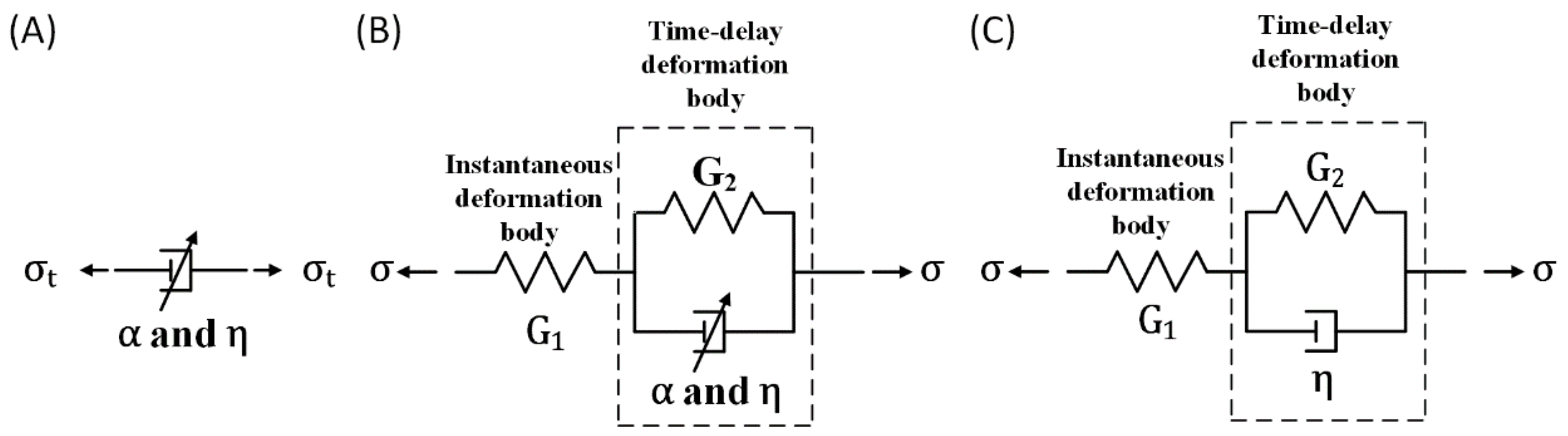
2. Fractional-Order Generalised Kelvin Model

The rheological element used to describe the fractional derivative is a damping element named Abel {Figure 1A} [28], whose constitutive relationship is as follows:
σ ( t ) = λ D α ε ( t ) 0 < α 1
where σ t and ε t are the stress and strain, respectively, at time t ; α is the order of fractional differentiation; λ = G 1 α η α , where G and η represent the shear modulus and the coefficient of viscosity, respectively; D represents the derivative operator with respect to time, t , D α = d α / d α t .
The fractional derivative element can be regarded as an ideal Newtonian liquid based on the assumption of α = 1 . Under the assumption of 0 < α < 1 , the fractional derivative element can be regarded as a fractional viscous body. This element can simulate the viscous behaviour of materials between ideal solids and liquids.
The fractional-order generalised Kelvin model {Figure 1B} is constructed by replacing the viscous element in the integer-order generalised Kelvin model {Figure 1C} with the Abel damping element, whose three-dimensional form of the constitutive equation is expressed as follows [23]:
P S i j = 2 Q e i j
σ i i = 3 K ε i i
where S i j ,   e i j ,   σ i i   and   ε i i are deviatoric stress tensor, deviatoric strain tensor, spherical stress tensor and spherical strain tensor, respectively; P   and   Q are viscoelastic differential operators, which are expressed as follows:
P = G 1 + G 2 + λ D α
Q = G 1 G 2 + λ G 1 D α
where G 1 and G 2 are the shear moduli; K is the bulk modulus and λ = G 2 1 α η α .

3. Viscoelastic Solutions for Surface Settlement under Vertically Distributed Loads

3.1. Elastic Solutions

The displacement of a half-space elastic body under a vertically distributed load on the boundary is calculated based on the Boussinesq displacement solution of a half-space elastic body under concentrated force [29]. When there is a normally concentrated force, P , acting on the surface origin 0 , 0 , the vertical displacement of the point x , y on the surface of ground is given as follows:
w M = ( 1 μ 2 ) P π E x 2 + y 2
where E is the modulus of elasticity and μ is the Poisson’s ratio.
By integration, the settlement, w x , y (vertical displacement), at any point x , y on the surface when the vertically distributed load, p ξ , ζ , is applied to the half-space elastomer and can be derived as:
w ( x , y ) = 1 μ 2 π E A p ( ξ , ς ) ( x ξ ) 2 + ( y ς ) 2 d ξ d ς
where A is the area where the load acts; p ξ , ζ is the load distribution function.
Let F x , y = A p ξ , ζ / x ξ 2 + y ζ 2 d ξ d ζ . When the distribution form of the load, p ξ , ζ , and the position of the point required to calculate the settlement are known, F x , y is only related to the coordinate position x , y , but unrelated to the elastic modulus, E , and the Poisson’s ratio, μ . Therefore, F x , y does not change when using the correspondence principle [25] to derive the viscoelastic solutions. Moreover, according to the correspondence principle, it is also necessary to express the elastic modulus, E , and Poisson’s ratio, μ , in Equation (7) in terms of the shear modulus, G , and bulk modulus, K :
w ( x , y ) = F ( x , y ) 4 π 1 G + 3 3 K + G

3.2. Viscoelastic Solutions

Applying the Laplace transform [25] separately to Equations (4) and (5):
L P = P ¯ s = G 1 + G 2 + λ s α
L Q = Q ¯ ( s ) = G 1 G 2 + λ G 1 s α
When the Laplace transform is performed on Equation (8), based on the requirements of the corresponding principle, G in Equation (8) should be replaced by Q ¯ / P ¯ , which can be expressed as follows:
w ¯ ( x , y , s ) = F ( x , y ) 4 π 1 G 1 s + 1 G 2 + λ s α s + 3 ( 3 K + G 1 ) s + 3 G 1 2 ( 3 K + G 1 ) [ 3 K ( G 1 + G 2 + λ s α ) + G 1 ( G 2 + λ s α ) ] s
where s is the parameter involved in the Laplace transform.
Applying the inverse Laplace transform to Equation (11), the settlement of any point x , y on the surface at a time, t , when the vertically distributed load, p ξ , ζ , acts on the fractional-generalised Kelvin half-space body is expressed as follows:
w ( x , y , t ) = F ( x , y ) 4 π 1 G 1 + 1 G 2 1 E α t α τ 1 + 3 3 K + G 1 + 3 G 1 2 ( 3 K + G 1 ) 3 K G 1 + 3 K G 2 + G 1 G 2 1 E α t α τ 2
where τ 1 = λ / G 2 , τ 2 = 3 K + G 1 λ / 3 K G 1 + 3 K G 2 + G 1 G 2 ; E · is the Mittag-Leffler function of a single parameter expressed as follows:
E α ( z ) = 0 z n Γ ( 1 + α n )
where Γ · is the Gamma function defined as Γ z = 0 t z 1 e t d t   and   R e z > 0 .

3.3. Analysis of Viscoelastic Solutions

F x , y > 0 when p ξ , ζ > 0 , if 0 < α 1 , the function, E α t α / τ , is completely monotonic for t 0 , , implying that d E α t α / τ / d t 0 and d 2 E α t α / τ / d t 2 0 [30]. Therefore, because d w x , y , t / d t 0 and d 2 w x , y , t / d t 2 0 , the settlement function, ω x , y , t , given by Equation (12), is a monotonically increasing and upwardly convex function at t 0 , . The instantaneous settlement, w x , y , 0 , at t = 0 is the minimum value:
w ( x , y , 0 ) = F ( x , y ) 4 π 1 G 1 + 3 3 K + G 1
Equation (14) is the same as Equation (8), and Equation (14) becomes Equation (8) when G 1 is replaced with G . This is because when t = 0 , the time-delay deformation body, which is composed of the Abel damping element and the elastic element, G 2 , connected in parallel, does not produce instantaneous deformation, and only the elastic element, G 1 , connected in series with it produces instantaneous elastic deformation. Thus, the instantaneous settlement is only related to the position coordinates x , y , G 1 and K , independent of α , G 2 and η .
Equation (12) shows that the settlement, w x , y , t , of each point also increases with an increase in t , and when t + , w x , y , + is a finite value that is the maximum value of settlement, whose value is as follows:
w ( x , y , + ) = F ( x , y ) 4 π 1 G 1 G 2 G 1 + G 2 + 3 3 K + G 1 G 2 G 1 + G 2
Equation (15) can be obtained by replacing G in Equation (8) with G 1 G 2 / G 1 + G 2 . This is because the Abel damping element does not work when t + , and only the two elastic elements G 1 and G 2 connected in series work, which is equivalent to an elastic element. When represented by an elastic element, G , it can be proved that G = G 1 G 2 / G 1 + G 2 . Therefore, the ultimate settlement is related to the elastic element’s G 1 and G 2 , which are independent of α and η in the damping element.

4. Parametric Analysis and Parametric-Sensitivity Analysis

The previous section shows that the creep described by the fractional-order generalised Kelvin model is the stable creep and Equations (14) and (15) show the functional relationship between instantaneous and ultimate settlements and each parameter; however, the influence of each parameter on the creep process cannot be intuitively observed from this function. Therefore, a specific example is used to analyse the influence of each parameter on the settlements at different moments.
Here, a rectangular area of a half-space viscoelastic surface is subjected to a uniform load of 1 MPa (Figure 2), and a set of basic parameters (Table 1) are selected according to the applicable parameters in the literature [24]. One of the parameters is increased by 20%, 40% and 60%, decreased by 20%, 40% and 60%, and the other parameters are kept constant, which allows the effect of each parameter on creep displacement to be studied.
For the given load distribution form in this example, the elastic and viscoelastic solutions of surface settlements are still calculated by Equations (8) and (12). F x , y in the equation is given as follows:
F ( x , y ) = p 0 a 1 l n a 3 + b 1 a 4 + b 3 + a 2 l n a 3 + b 2 a 4 + b 4 + a 3 l n a 1 + b 1 a 2 + b 3 + a 4 l n a 1 + b 3 a 2 + b 4
where a 1 = b / 2 x , a 2 = b / 2 + x , a 3 = a / 2 y , a 4 = a / 2 + y , b 1 = a 1 2 + a 3 2 , b 2 = a 2 2 + a 3 2 , b 3 = a 1 2 + a 4 2 , b 4 = a 2 2 + a 4 2 , where a and b are the lengths of the rectangle along the x and y axes, respectively; p 0 is the uniformly distributed load acting on the surface, which is 1   M P a for this example.
Because the viscoelastic solutions of the settlements, w x , y , t and F x , y , are linearly related, the settlements at different locations have the same variation law with time; for convenience, we only selected the settlements at the centre of the rectangle for analysis.

4.1. Effect of Differential Order
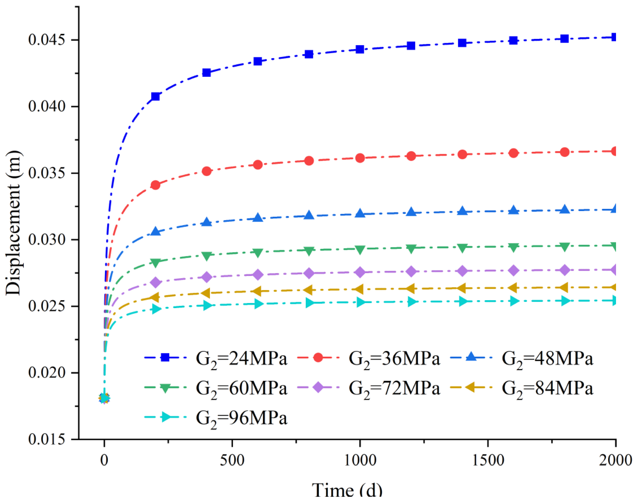
 α

First, the order α of the differential is increased by 20%, 40% and 60% and decreased by 20%, 40% and 60%, while other parameters are kept constant. Figure 3 shows the settlements at the centre of the rectangle with time for different α. The figure shows that the settlements contain two stages, instantaneous settlement and deceleration creep, and the change in order α has no effect on the instantaneous settlement at t = 0 and the ultimate settlement at t + , which is consistent with the law described in the analysis of viscoelastic solutions above. Moreover, Figure 3B shows that there is a demarcation point for different α that divides the creep curve into two stages: in the first stage, the settlement’s value decreases at the same moment as α increases; in the second stage, the settlement’s value increases at the same moment as α increases. The peculiar law is attributed to the Abel damping element, an intermediate between the ideal solid α = 0 and the Newtonian fluid α = 1 , which allows the fractional-order model to describe a wider range of rheological properties of the soil or rock than the integer-order model α = 1 . This phenomenon is consistent with the results of the literature [22,23,24]. The smaller the value of α , the longer the time required to reach a steady state. For α = 1, 0.8, 0.7, 0.6, 0.5, 0.4, 0.3 and 0.2, the times required for the basic stabilisation of settlements are 130 , 2 × 10 4 ,   10 5 ,   8 × 10 5 ,   10 7 ,   5 × 10 8 ,   2 × 10 11   and   4 × 10 16   d , respectively.

4.2. Influence of Shear Modulus ( G 1 )

The shear modulus, G 1 , is increased by 20%, 40% and 60% and decreased by 20%, 40% and 60%, while other parameters are kept constant. Figure 4 shows the settlements at the centre of the rectangle with time for different G 1 . The analysis of viscoelastic solutions in the previous section shows that G 1 influences the instantaneous and ultimate settlements, and Figure 4 shows that the larger G 1 is, the smaller the instantaneous and ultimate settlements. Moreover, in the creep deceleration stage of 0 < t < + , the settlement value and the change amplitude of settlements also decrease as G 1 increases, and the change amplitude of settlements is also related to the time, t. When G 1 increases from 24 to 96 MP, the instantaneous settlements are 0.0360, 0.0262, 0.0212, 0.0181, 0.0160, 0.0144 and 0.0131 m, while the amplitudes of the change in settlements are 54.14%, 27.62%, 17.13%, 11.6%, 8.84% and 7.18%, respectively. In addition, the ultimate settlements are 0.0475, 0.0379, 0.0331, 0.0302, 0.0282 m, 0.0268 and 0.0257 m, with corresponding amplitudes of the change in settlements of 31.79%, 15.89%, 9.60%, 6.62%, 4.64% and 3.64%, respectively.

4.3. Influence of Shear Modulus ( G 2 )

The shear modulus, G 2 , is increased by 20%, 40% and 60% and decreased by 20%, 40% and 60%, while other parameters are kept constant. Figure 5 shows the settlements at the centre of the rectangle with time for different G 2 . The analysis of viscoelastic solutions in the previous section shows that G 2 does not affect the instantaneous settlement but affects the ultimate settlement, and the larger G 2 is, the smaller the ultimate settlement value. Moreover, Figure 5 shows that in the creep deceleration stage of 0 < t < + , the settlement values and the amplitudes of the change in the settlement also decrease with the increase of G 2 . When G 2 increases from 24 to 96 MP, the ultimate settlements are 0.0475, 0.0379, 0.0331, 0.0302, 0.0282, 0.0268 and 0.0257 m, with corresponding amplitudes of the change in the settlement of 31.79%, 15.89%, 9.60%, 6.62%, 4.64% and 3.64%.

4.4. Effect of Viscosity Coefficient η

The viscosity coefficient, η , is increased by 20%, 40% and 60% and decreased by 20%, 40% and 60%, while other parameters are kept constant. Figure 6 shows the settlements at the centre of the rectangle with time for different η . The analysis of viscoelastic solutions in the previous section shows that η does not affect the instantaneous and ultimate settlements. However, Figure 6 shows that the viscosity coefficient, η, affects the settlement rate, and the smaller the value of η, the less the time it takes for the settlement to reach a steady state. The calculation shows that for η increasing from 400 to 1600   MPa · d , the time required to reach the ultimate settlement at t + are, respectively, 4 × 10 6 , 6 × 10 6 , 8 × 10 6 , 1.05 × 10 6 , 1.25 × 10 7 , 1.45 × 10 7 and 1.65 × 10 7   d . Moreover, the change in η has a lower influence on the change amplitude of settlement than other parameters. When t = 100   d , the settlements are 0.0285, 0.0282, 0.0279, 0.0276, 0.0274, 0.0273 and 0.0271 m, with corresponding amplitudes of the change in the settlement of only 1.25%, 1.01%, 0.86%, 0.76%, 0.67% and 0.61%.

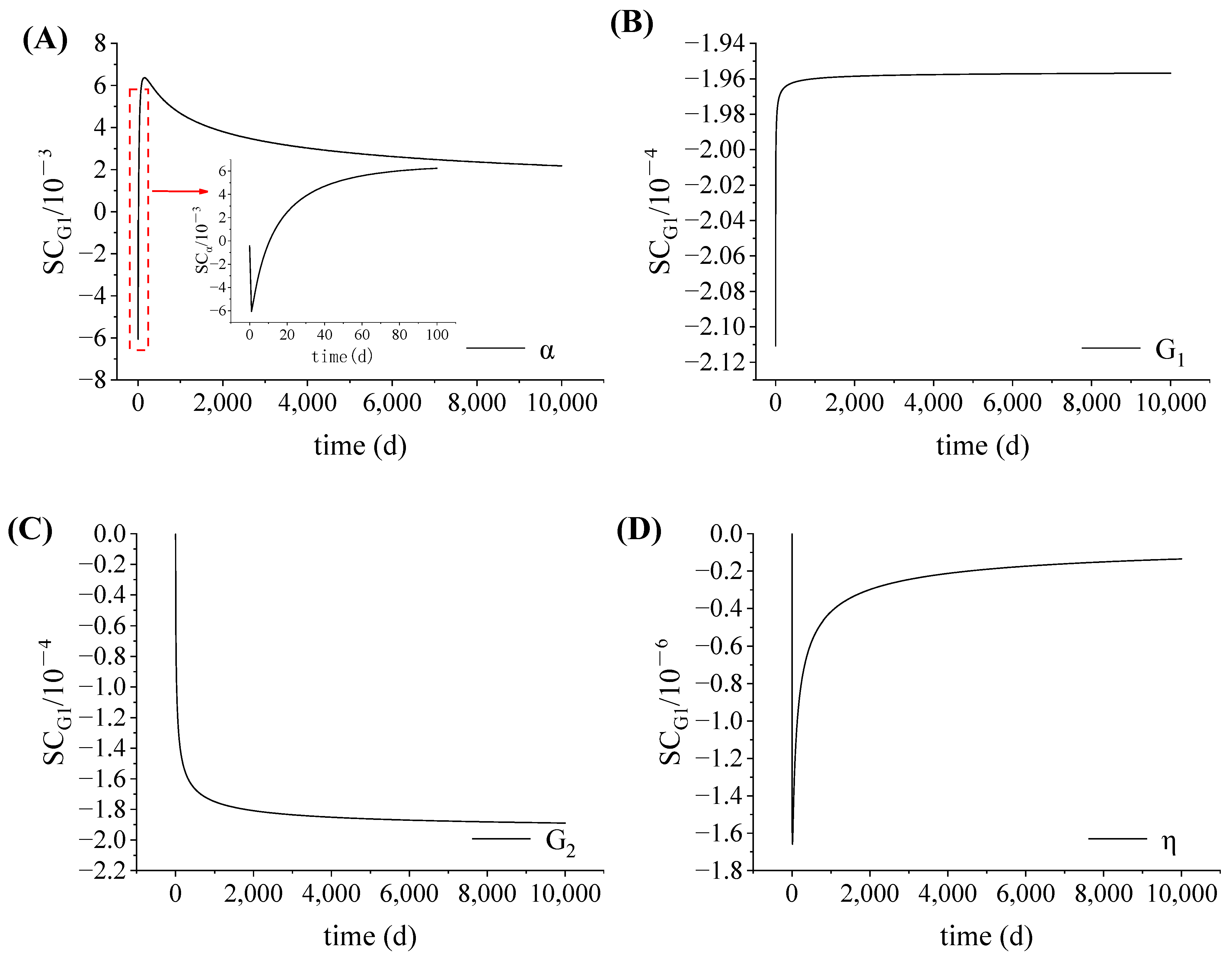
4.5. Parametric-Sensitivity Analyses

During the analysis of the aforementioned parameters, we discovered that the change in each parameter has a different amplitude of influence on the settlement. The sensitivity coefficient (SC) was used to analyse and compare the influence of each parameter on the settlement [31]. SC denotes the rate at which the model output value changes due to a slight change in the parameter value. In mathematics, SC is the partial derivative of the dependent variable for each independent variable, and it is therefore expressed in this study as a first-order partial derivative of the settlement function, w x , y , t , with respect to α , G 1 , G 2 and η :
S C α = w ( x , y , t ) α = F ( x , y ) 4 π 1 G 2 1 Ψ 1 + Φ 1 1 Ψ 2 S C G 1 = w ( x , y , t ) G 1 = F ( x , y ) 4 π 1 G 1 2 3 3 K + G 1 2 + Φ 2 1 E α t α τ 2 Φ 1 1 Ψ 3 S C G 2 = w ( x , y , t ) G 2 = F ( x , y ) 4 π 1 G 2 2 1 E α t α τ 1 α G 2 2 1 Ψ 4 Φ 3 1 E α t α τ 2 Φ 1 1 Ψ 5 S C η = w ( x , y , t ) η = F x , y 4 π 1 G 2 1 Ψ 6 Φ 1 1 Ψ 7
where Ψ 1 = n t α τ 1 n l n t G 2 η Γ 1 + α n n t α τ 1 n 0 t α n e t ln t d t Γ 1 + α n 2 , Ψ 2 = n t α τ 2 n l n t G 2 η Γ 1 + α n n t α τ 2 n 0 t α n e t ln t d t Γ 1 + α n 2 , Ψ 3 = t α τ 2 n Γ 1 + α n 9 n K 2 3 K + G 1 3 K G 1 + 3 K G 2 + G 1 G 2 , Ψ 4 = n t α τ 1 n Γ 1 + α n , Ψ 5 = n t α τ 2 n Γ 1 + α n α 1 3 K G 1 + 3 α K G 2 + α G 1 G 2 3 K G 1 + 3 K G 2 + G 1 G 2 G 2 , Ψ 6 = t α τ 1 n α n η Γ 1 + α n , Ψ 7 = t α τ 2 n α n η Γ 1 + α n , Φ 1 = 3 G 1 2 3 K + G 1 3 K G 1 + 3 K G 2 + G 1 G 2 , Φ 2 = 18 K G 1 2 G 2 + 27 K 2 G 1 2 + 54 K 2 G 1 G 2 3 K + G 1 3 K G 1 + 3 K G 2 + G 1 G 2 2 , Φ 3 = 3 G 1 2 3 K G 1 + 3 K G 2 + G 1 G 2 2 .
The SCs of the parameters solved by the first-order partial derivatives produce large errors after 100   d due to the influence of computational errors. Therefore, the SCs are calculated using this method for the first 100   d , and thereafter they are approximated using the differential method as follows:
S C j t = w t + Δ X j w t Δ X j
where w t is the creep displacement corresponding to the basic parameter; Δ X j is the j th mechanical parameter change in the base parameter; w t + Δ X j is the creep displacement corresponding to the change in the j th mechanical parameter.
Equation (18) is used to compute the four mechanical parameters after increasing them by 1%. Figure 7 shows the results of the SCs for each parameter.
Figure 7A shows that when 0 t < 13   d , SC < 0 and when t > 13   d , SC > 0, indicating that the settlements are negatively correlated with α before 13   d , and positively correlated with α after 13   d , which also proves the law obtained from the previous analysis of the effect of differential order α on settlement: there is a point on the creep curve that divides it into two stages, and the law of increase and decrease in settlements in the two stages is opposite to the increase in α . Moreover, S C α = 0 when t = 0 and t + , which also proved the law that the change in α has no effect on the instantaneous and final settlements.
Figure 7B,C show that S C G 1 < 0 and S C G 2 0 , indicating that the settlements are negatively correlated with G 1 and G 2 . Moreover, S C G 1 decreases gradually with time, t, and tends to be stable, whereas S C G 2 increases gradually with time, t, and tends to be stable, and when t + , S C G 1 = S C G 2 = 1.995 × 10 4 , thus the changes in G 1 and G 2 affect the final settlement. S C η = 0 when t = 0 and t + , thus the change in η does not affect the instantaneous and final settlement.
Figure 7D shows that S C η < 0 , indicating that the settlements are negatively correlated with η . In addition, S C η increases first and then decreases with time t , implying that the influence of η on settlements first increases and then decreases.
By calculation, 6.2 × 10 3 S C α 6.4 × 10 3 , 2.1 × 10 4 S C G 1 1.995 × 10 4 , 1.995 × 10 4 S C G 2 0 and 1.7 × 10 6 S C η 0 . Thus, α is the most sensitive to the settlement effects, followed by G 1 and G 2 , while η is the least sensitive. Therefore, significant attention should be given to α , G 1 and G 2 when the displacement inverse analysis method is used to invert the geotechnical parameters.

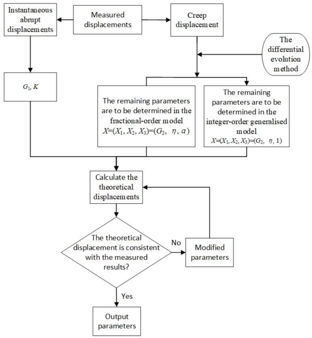
5. Method of Determining Parameters by Field Experiments

The field-bearing plate test is a method for determining the deformation parameters of rock masses, and it is also commonly used to execute field creep tests due to its simple test procedure and easy operation. The bearing plate test is theoretically based on Boussinesq’s solution for local forces on the surface of a uniform, continuous and isotropic semi-infinite elastomer [8].
The bearing plate test can be divided into rigid and flexible bearing plate tests according to the stiffness of the bearing plate and the size of the elastic modulus of the rock mass. In the rigid bearing plate test, the rock body is considered flexible while the bearing plate is rigid, and the vertical displacement generated at each point of the rock body below the contact with the bearing plate is the same; however, the normal pressure between the bearing plate and the rock body is not uniformly distributed. In the flexible bearing plate test, the bearing plate is considered flexible, and the normal pressure between the bearing plate and the rock mass is uniform; however, the vertical displacement produced by the rock mass below the bearing plate is not uniform.
The displacement solutions for the two cases of circular flexible and rigid bearing plates are derived below, based on the integer- and fractional-order generalised Kelvin models. The creep test results are then used to identify each parameter in the model using the displacement inverse analysis method.

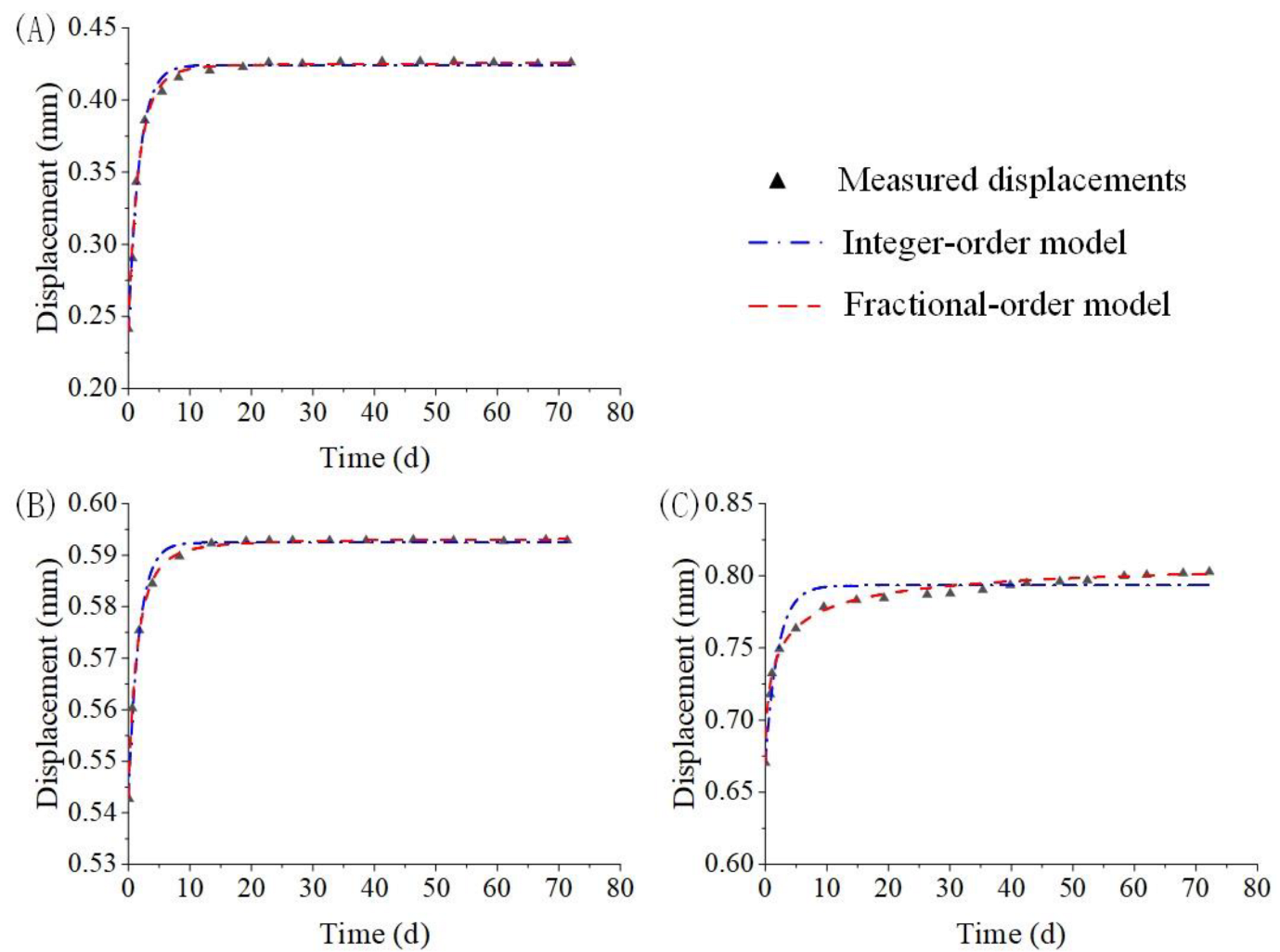
5.1. Parameter Identification of the Circular Flexible Bearing Plate Test

Jinping I Hydropower Station uses flexible bearing plates with a diameter of 105 cm (effective output size of 100 cm) at the dam site to conduct creep tests on the bearing plates on site [8].
A displacement measuring instrument was installed at the edge of a circular flexible bearing plate, and the elastic and viscoelastic solutions of settlement at the measuring point were calculated using Equations (8) and (12), in which F x , y is expressed in polar coordinates as follows:
F x , y = F r = R 0 = 4 p R 0
where R 0 is the radius of the pressure plate, r is the pole diameter, and p is the uniform load under the bearing plate.
Figure 8 shows the creep curves of the rock mass at different loading stages. The figure shows that the rock mass has obvious instantaneous abrupt displacement and tends to be stable after creep with a gradually decreasing rate. Therefore, the rock mass can be regarded as a viscoelastic body, and its deformation can be analysed using the fractional-order generalised Kelvin model, including instantaneous and creep deformations.
The process of parameter inversion is shown in Figure 9. First, based on the elastic displacement formula at the edge of a circular flexible bearing plate, the elastic modulus E 0 of the rock mass can be obtained from the instantaneous deformation, w 0 , at the edge of the bearing plate:
E 0 = 4 p R 0 ( 1 μ 2 ) π w 0
The shear and bulk moduli of the rock mass are then expressed as follows:
G 1 = E 0 2 ( 1 + μ ) , K = E 0 3 ( 1 2 μ )
Second, other parameters, G 2 , η and α , in the fractional-order model are inverted according to the measured creep displacement. The objective function is established by the residuals of the measured displacement, w t i , and the calculated displacement, w X , t i , at moment t i , and the objective function in the form of the sum of squares is expressed in this study as follows:
F ( X ) = i = 1 N [ w ( t i ) w X , t i ] 2
where X is the design variable expressed as follows:
X = ( X 1 , X 2 , X 3 ) = ( G 2 , η , α )
where N is the number of measured displacements.
In this study, the set of X that minimises Equation (22) is obtained using the differential evolution method [32], and X is the determined parameter. This degenerates to the case of using the integer-order generalised Kelvin model if α = 1 , and the parameters G 2 and η can be obtained using the differential evolution method.
In this study, the coefficient of determination, R 2 , is applied to evaluate the performance of the aforementioned two models.
R 2 = 1 i = 1 N w t i w X , t i 2 i = 1 N w t i w ¯ 2
where w ¯ is the average value of the measured displacements.
Table 2 and Table 3 show the parameters of the rheological models obtained under different loading conditions, based on the above two-step inversion analysis process. The theoretical displacement curves under different stress levels are then obtained by substituting the inversion analysis parameters into the corresponding analytical equations. Figure 10 shows the comparisons between the theoretical displacement curves based on the two rheological models and the measurements obtained under different stress levels.
Figure 10 shows that the creep curves described by the integer-order model have a faster growth rate in the deceleration creep phase, so it will quickly reach stability, and the results have a serious error when considered in the context of the field-measured data; moreover, the error increases with an increase in the stress level, and the calculated displacement of the final creep is smaller than the measured displacement. The creep curves in the deceleration creep stage for the fractional-order model are consistent with the measurements obtained at different stress levels, which can better describe the creep process of the rock mass. Because the fractional-order model has the additional parameter, α, which can adjust the rate of the deceleration creep phase compared with the traditional integer-order model, this enables the creep rate to be adjusted over a wider range. The determination coefficients of the integer-order model and the fractional-order model are shown in Table 2, and the fitting accuracy of the latter is significantly better than that of the former. Moreover, the coefficients of determination between the calculated displacements of the fractional-order model and measured displacements are all greater than 0.99 at different levels, with a high correlation; thus, the fractional-order model can also describe the creep behaviour of the rock well at high-stress levels.

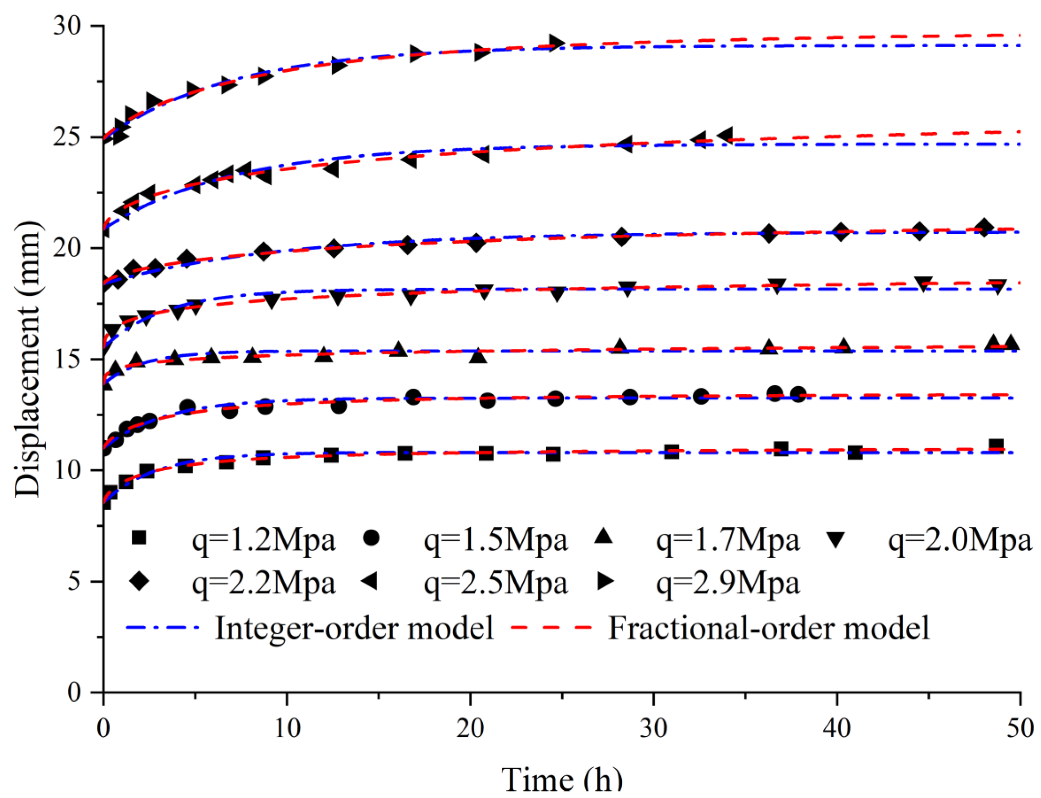
5.2. Parameter Identification of Circular Rigid Bearing Plate Test

A circular rigid pressure-bearing plate with an area of 2000 cm2 was used to test the shale section on the downstream side of the second stage hoist foundation of the Tectonic Beach Hydropower Station for compression creep [26]. The displacement measuring instrument was situated beneath the circular rigid bearing plate, and the load was applied by the jack above the bearing plate. The stress distribution transferred to the rock by the circular rigid bearing plate is as follows [33]:
p ( r ) = P 2 π r R 0 2 r 2
where P is the total pressure on the bearing plate, P = π R 0 2 q ; q is the normal uniform load applied by the jack. The elastic and viscoelastic solutions of settlement at the measuring point are calculated using Equations (7), (12) and (25), in which F x , y is expressed in polar coordinates as follows:
F x , y = F ( 0 r R 0 ) = π 2 R 0 q 2
The results of the rheological model parameter inversions of the rock are obtained using the same parameter inversion method as in the previous section (Table 4 and Table 5). Figure 11 also shows the comparisons between the theoretical displacement curves of the two models and the measurements obtained.
Figure 11 shows that both the calculated displacements based on the integer- and fractional-order models can be consistent with the measurements obtained at different stress levels; however, as time increases, the creep deformations predicted by the integer-order model are smaller than those of the fractional-order model. Table 4 and Table 5 show the coefficients of determination of the calculated displacements and the measurements obtained for the two models. The fractional-order model’s coefficients of determination are larger than those of the integer-order model at different stress levels, and the fractional-order model’s coefficients of determination are greater than 0.95. Therefore, the model’s theoretical displacements correlate highly with the measurements obtained and can better describe and predict the rock’s creep deformation.

6. Conclusions

This study develops the fractional-order generalised Kelvin model by replacing the viscous elements in the classical integer-order generalised Kelvin model with the Abel damping element. The viscoelastic solutions of a half-space viscoelastic body subjected to arbitrarily distributed loads are solved for the fractional-order model. In addition, the function of the settlement is a monotonically increasing function with upper and lower bounds, demonstrating that the model describes the stable creep and verifies the unity of the creep equation and the elastic deformation equation for t = 0 and t + .
The fractional-order generalised Kelvin model has one more parameter, the differential order, α , than the integer-order generalised Kelvin model that can regulate the rate of the decremental phase, according to the parametric and parametric-sensitivity analyses of the four parameters in the fractional-order generalised Kelvin model. Therefore, the model is more flexible and can describe a wider variety of rheological properties of viscoelastic bodies, and this parameter is more sensitive to displacement than the other three parameters.
The fractional- and integer-order generalised Kelvin models are used to fit the experimental results of the two groups of field-bearing plate creep experiments. The results show that the fractional-order generalised Kelvin model has a better correlation than the integer-order generalised Kelvin model and can better fit the rock’s creep curve.

Author Contributions

A.L. conceived and designed the study. B.H. derived the formulas and wrote the programs. B.H. wrote the paper. A.L. and N.Z. reviewed the edited manuscript. All authors have read and agreed to the published version of the manuscript.

Funding

The study is supported by the National Natural Science Foundation of China (U2106224, 51974124) and the Fundamental Research Funds for the Central Universities (2020MS027).

Institutional Review Board Statement

Not applicable.

Informed Consent Statement

Not applicable.

Data Availability Statement

Some or all data, models, or code generated or used during the study are available from the corresponding author by request.

Acknowledgments

We thank the staff at the same laboratory. We also would like to thank the reviewers for their constructive comments.

Conflicts of Interest

The authors declare no conflict of interest.

References

  1. Maheshwari, P.; Viladkar, M.; Kumar, A. Experimental evaluation of nonlinear Kelvin model constants from triaxial test data. Int. J. Geotech. Eng. 2011, 5, 363–371. [Google Scholar] [CrossRef]
  2. Zhao, D.; Jia, L.; Wang, M.; Wang, F. Displacement prediction of tunnels based on a generalised Kelvin constitutive model and its application in a subsea tunnel. Tunn. Undergr. Space Technol. 2016, 54, 29–36. [Google Scholar] [CrossRef]
  3. Huang, M.; Zhan, J.W.; Xu, C.S.; Jiang, S. New Creep Constitutive Model for Soft Rocks and Its Application in the Prediction of Time-Dependent Deformation in Tunnels. Int. J. Geomech. 2020, 20, 04020096. [Google Scholar] [CrossRef]
  4. Wei, Y.; Chen, Q.; Huang, H.; Xue, X. Study on creep models and parameter inversion of columnar jointed basalt rock masses. Eng. Geol. 2021, 290, 106206. [Google Scholar] [CrossRef]
  5. Li, Y.-P.; Wang, Z.-Y.; Ding, X.-L. Model identification for rheological load test curve and its application. J. Univ. Pet. China Nat. Sci. Ed. 2005, 29, 73–77. [Google Scholar]
  6. Yang, W.; Zhang, Q.; Li, S.; Wang, S. Estimation of in situ viscoelastic parameters of a weak rock layer by time-dependent plate-loading tests. Int. J. Rock Mech. Min. Sci. 2014, 66, 169–176. [Google Scholar] [CrossRef]
  7. Xiong, S.; Zhou, H.; Zhong, Z. Study of methodology of plate-loading creep test of rock mass. Chin. J. Rock Mech. Eng. 2009, 28, 2121–2127. [Google Scholar]
  8. Huang, S.; Ding, X.; He, J.; Xiong, S. Analytical solution for rock mass bearing plate rheological tests based on a novel viscoelastic combination model. Eur. J. Environ. Civ. Eng. 2022, 26, 3204–3218. [Google Scholar] [CrossRef]
  9. Zhou, F.-X.; Wang, L.-Y.; Liu, Z.-Y.; Zhao, W.-C. A viscoelastic-viscoplastic mechanical model of time-dependent materials based on variable-order fractional derivative. Mech. Time Depend. Mater. 2021, 26, 699–717. [Google Scholar] [CrossRef]
  10. Lewandowski, R.; Chorążyczewski, B. Identification of the parameters of the Kelvin–Voigt and the Maxwell fractional models, used to modeling of viscoelastic dampers. Comput. Struct. 2010, 88, 1–17. [Google Scholar] [CrossRef]
  11. Beltempo, A.; Zingales, M.; Bursi, O.S.; Deseri, L. A fractional-order model for aging materials: An application to concrete. Int. J. Solids Struct. 2018, 138, 13–23. [Google Scholar] [CrossRef]
  12. Meng, R.; Yin, D.; Yang, H.; Xiang, G. Parameter study of variable order fractional model for the strain hardening behavior of glassy polymers. Phys. A Stat. Mech. Its Appl. 2020, 545, 123763. [Google Scholar] [CrossRef]
  13. Liu, F.; Wang, J.; Long, S.; Zhang, H.; Yao, X. Experimental and modeling study of the viscoelastic-viscoplastic deformation behavior of amorphous polymers over a wide temperature range. Mech. Mater. 2022, 167, 104246. [Google Scholar] [CrossRef]
  14. Xiang, G.; Yin, D.; Cao, C.; Gao, Y. Fractional description of creep behavior for fiber reinforced concrete: Simulation and parameter study. Constr. Build. Mater. 2022, 318, 126101. [Google Scholar] [CrossRef]
  15. Wu, F.; Zhang, H.; Zou, Q.; Li, C.; Chen, J.; Gao, R. Viscoelastic-plastic damage creep model for salt rock based on fractional derivative theory. Mech. Mater. 2020, 150, 103600. [Google Scholar] [CrossRef]
  16. Ding, X.; Zhang, G.; Zhao, B.; Wang, Y. Unexpected viscoelastic deformation of tight sandstone: Insights and predictions from the fractional Maxwell model. Sci. Rep. 2017, 7, 11336. [Google Scholar] [CrossRef] [Green Version]
  17. Sun, H.-Z.; Zhang, W. Analysis of soft soil with viscoelastic fractional derivative Kelvin model. Rock Soil Mech. 2007, 28, 1983–1986. [Google Scholar]
  18. Zhou, H.W.; Wang, C.P.; Han, B.B.; Duan, Z.Q. A creep constitutive model for salt rock based on fractional derivatives. Int. J. Rock Mech. Min. Sci. 2011, 48, 116–121. [Google Scholar] [CrossRef]
  19. Zhou, H.W.; Liu, D.; Lei, G.; Xue, D.J.; Zhao, Y. The Creep-Damage Model of Salt Rock Based on Fractional Derivative. Energies 2018, 11, 2349. [Google Scholar] [CrossRef] [Green Version]
  20. Gao, Y.; Yin, D. A full-stage creep model for rocks based on the variable-order fractional calculus. Appl. Math. Model. 2021, 95, 435–446. [Google Scholar] [CrossRef]
  21. Liu, N.; Zhu, W.S.; Li, X.J. Analysis of finite element viscoelastic displacement based on Kelvin model. Adv. Mater. Res. 2008, 33, 413–420. [Google Scholar] [CrossRef]
  22. Qin, W. Deformation analysis of fractional derivative Kelvin model foundation under horizontal concentrated force. Chin. J. Appl. Mech. 2021, 38, 2132–2136. [Google Scholar]
  23. Li, X.-M.; Zhang, Q.-Q.; Feng, R.-F.; Qian, J.-G.; Wei, H.-W. Long-Term Deformation Analysis for a Vertical Concentrated Force Acting in the Interior of Fractional Derivative Viscoelastic Soils. Int. J. Geomech. 2020, 20, 04020040. [Google Scholar] [CrossRef]
  24. Zhu, H.-H.; Liu, L.-C.; Pei, H.-F.; Shi, B. Settlement analysis of viscoelastic foundation under vertical line load using a fractional Kelvin-Voigt model. Geomech. Eng. 2012, 4, 67–78. [Google Scholar] [CrossRef]
  25. Lee, E. Stress analysis in visco-elastic bodies. Q. Appl. Math. 1955, 13, 183–190. [Google Scholar] [CrossRef] [Green Version]
  26. Chen, J.; Jian, B.; Zuo, C.; Yu, X. In-situ rheological test and study of soft rock at Goupitan Hydropower Station. Yangtze River 2015, 46, 48–51. [Google Scholar]
  27. Sakurai, S. Back Analysis in Rock Engineering; CRC Press: Boca Raton, FL, USA, 2017. [Google Scholar]
  28. Koeller, R.C. Applications of Fractional Calculus to the Theory of Viscoelasticity. J. Appl. Mech. 1984, 51, 299–307. [Google Scholar] [CrossRef]
  29. Lurie, A.I.; Belyaev, A. Theory of Elasticity; Springer: Berlin/Heidelberg, Germany, 2010. [Google Scholar]
  30. Miller, K.S.; Samko, S.G. Completely monotonic functions. Integral Transform. Spec. Funct. 2001, 12, 389–402. [Google Scholar] [CrossRef]
  31. Gu, R.R.; Li, Y. River temperature sensitivity to hydraulic and meteorological parameters. J. Environ. Manag. 2002, 66, 43–56. [Google Scholar] [CrossRef]
  32. Opara, K.R.; Arabas, J. Differential Evolution: A survey of theoretical analyses. Swarm Evol. Comput. 2019, 44, 546–558. [Google Scholar] [CrossRef]
  33. Balakrishna, C.K.; Murthy, B.R.S.; Nagaraj, T.S. Stress distribution beneath rigid circular foundations on sands. Int. J. Numer. Anal. Methods Geomech. 1992, 16, 65–72. [Google Scholar] [CrossRef]
Figure 1. Schematic of the rheological models: (A) Abel damping element, (B) Fractional-order generalised Kelvin model, (C) Integer-order generalised Kelvin model.
Applsci 13 00648 g001
Figure 2. Load distribution range.
Applsci 13 00648 g002
Figure 3. Creep curves under different α: (A) 0 t 2000   d , (B) 0 t 80   d .
Applsci 13 00648 g003
Figure 4. Creep curves under different G1.
Applsci 13 00648 g004
Figure 5. Creep curves under different G2.
Applsci 13 00648 g005
Figure 6. Creep curves under different η.
Applsci 13 00648 g006
Figure 7. Sensitivity analysis: (A) SC of differential order, α , (B) SC of shear modulus, G 1 , (C) SC of shear modulus, G 2 and (D) SC of viscosity coefficient, η .
Applsci 13 00648 g007
Figure 8. Creep curves of rock mass at different loading stages of circular flexible pressure-bearing plates.
Applsci 13 00648 g008
Figure 9. The process of parameter inversion.
Applsci 13 00648 g009
Figure 10. Comparisons between the theoretical displacements based on the two rheological models and the measured results: (A) p = 2   MPa , (B)   p = 3   MPa and (C) p = 4   MPa .
Applsci 13 00648 g010
Figure 11. Comparisons between the theoretical displacements based on the two rheological models and the measured results.
Applsci 13 00648 g011
Table 1. Basic parameters of the fractional-order generalised Kelvin model.
ItemValue
Shear modulus G 1 (MPa)60
Shear modulus G 2 (MPa)60
Bulk modulus K (MPa)80
Viscosity coefficient η (MPa·d)1000
Fractional differential order α 0.5
Table 2. Inverse analysis results based on the integer-order model.
p   M P a K   G P a G 1   G P a G 2   G P a η   G P a · h R 2
23.30871.98521.80813.26820.9929
32.20101.318010.401017.96020.9938
42.37601.42285.550911.55280.9401
Table 3. Inverse analysis results based on the fractional-order model.
p   M P a K   G P a G 1   G P a G 2   G P a η   G P a · h α R 2
23.30871.98521.79193.28020.94120.9941
32.20101.318010.204217.58200.86800.9993
42.37601.42284.669615.52690.53300.9932
Table 4. Inverse analysis results based on the integer-order model.
q   M P a K   G P a G 1   G P a G 2   G P a η   G P a · h R 2
1.234.7720.8656.13160.090.9631
1.533.7720.2670.69237.650.9602
1.730.2918.18112.89270.780.8177
2.031.8919.1381.20275.010.9228
2.229.6117.77100.54900.400.9653
2.529.6817.8169.40496.770.9385
2.928.8217.2973.28525.610.9785
Table 5. Inverse analysis results based on the fractional-order model.
q   M P a   K   G P a   G 1   G P a   G 2   G P a   η   G P a · h   α R 2  
1.234.7720.8649.95171.040.7070.9913
1.533.7720.2662.81277.650.7570.9833
1.730.2918.1874.1910000.3890.9526
2.031.8919.1355.89557.660.4960.9944
2.229.6117.7788.5010000.7860.9855
2.529.6817.8143.4210000.6130.9858
2.928.8217.2961.48633.920.8520.9827
Disclaimer/Publisher’s Note: The statements, opinions and data contained in all publications are solely those of the individual author(s) and contributor(s) and not of MDPI and/or the editor(s). MDPI and/or the editor(s) disclaim responsibility for any injury to people or property resulting from any ideas, methods, instructions or products referred to in the content.

