1. Introduction
With the development of modern manufacturing, the industrial environment is becoming more dynamic and complex. The deployment of mobile robots in different industrial areas emphasizes the tracking of robot targets as one of the important functions for monitoring and coordination in an unknown environment. Different techniques have been proposed for robot tracking.
Camera lens distortion correction, non-uniform light compensation techniques, a modified non-linear state estimator and an improved Matrox Meteor Frame-grabber were proposed around the year 2000 in the field of mobile robot tracking [
1,
2,
3]. Monitoring objects against the cluttered moving background and dynamic objects/intrusions moving through the scene are huge challenges in partial occlusion. Hongxin Wang’s team [
4] proposed a novel visual system model (STMD+) for small target motion detection to discriminate small targets from small target-like background features (named fake features). A novel technique for background subtraction based on the dynamic autoregressive moving average (ARMA) model was raised by Jian Li’s team [
5]. A motion-planning framework for urban autonomous driving at uncontrolled intersections was presented by Jeong and Yi [
6]. However, processing speed and anti-blocking properties of these deep learning (DL) methods have not been paid enough attention in the mobile robot tracking area.
To solve the underlying optimization problems, neural network (NN) based models, especially convolutional neural network (CNN) models, recurrent neural network (RNN) and graph neural network (GNN) models, can be adopted [
7]. Most of the research approaches with NN-based methodologies in target tracking problems have focused on solving filtering in target tracking, target drift and target loss and improving the tracking precision, especially in low-quality videos [
8,
9,
10]. In a dynamic scenario, we only have initially knowledge of the robot we want to track. The data set of the target robot in the indoor and outdoor environment may be collected for training. The robot will then be deployed in an unknown environment. However, during the maneuver of the robots, fast target motion and unknown interference items present in the scene might cause severe occlusion of the robot target. This imposes the major challenge in NN-based target tracking.
Various solutions have been proposed to resolve the occlusion problem. Wang and Yuille [
11] designed an end-to-end deep occlusion network (DOC) for estimating occlusion relations which enable better training and testing of deep networks for occlusion estimation. Ren et al. [
12] developed a computational model for figure/ground assignment in a complex natural scene. The model provided a feasible approach to bottom-up figure/ground assignment in natural images. Hoiem et al. [
13] raised an approach to recover the occlusion boundaries and depth ordering of free-standing structures in the scene. The research pointed out a research direction for single-image occlusion reasoning and the broader 3D scene understanding problem. Kotsia et al. [
14] addressed the effect of partial occlusion on facial expression recognition. They analyzed the way in which partial occlusion affects the recognition of facial expressions by human observers. Weiwei Zhang et al. [
15] developed a novel vehicle detection based on vehicle part-based proposals generation and Part Affinity Fields (PAFs)-based combination algorithm to solve the visual detection problem of occlusion in complex backgrounds. The designed algorithm improves the performance of accuracy, especially when vehicles are heavily occluded. Yuille and Liu [
16] provided a review of the strengths and weaknesses of Deep Nets for vision from 2018 to 2020. It was proven that even though real-world image sets are infinitely large and any data set (no matter how big) is hardly representative of real-world complexity, using a DL model for visual problems can solve specific visual tasks and has the potential for practical applications.
In view of the previous research, the following research questions are addressed in this paper: (1) whether the deep learning model tracking methods, Faster RCNN, SSD and YOLOv5, can adapt to various occlusion conditions and (2) to what extent occlusion could be handled in a specific environment. To address these issues, a training data set of the robot target under designated mobility and occlusion conditions needs to be constructed in our research. Different testing data sets are also created. We then focus on three recent versions of DL models, You Only Look Once (YOLO) model—YOLOv5, Faster Region Proposal Convolutional Neural Network (R-CNN) and Single Shot MultiBox Detector (SSD), and compare the performance of the three DL models in the robot target tracking. A Random Erasing method is proposed to generate some testing data to mimic random interference items that block the view of the target. Different dynamic occlusion variation situations have also been tested where part of the targets is out of range. The missing portion is about 10% to 30% of the target. The environment contains indoor and outdoor environments with different backgrounds.
The contributions of the article are summed up as follows: (1) We build three evaluation data sets for training and algorithm verification under single target tracking scenarios. (2) We construct three recent object detection models, which are Faster RCNN, SSD and YOLOv5. Comprehensive experiments are conducted to evaluate the detection performance with our data sets. (3) We design a Random Erasing method to create a new testing data set with various partial occlusions to verify the system performance. (4) We use image views from different angles, distances and surrounding environments to test the model performance. (5) We numerically analyze the adaptivity of the models against different degrees of occlusions through experiments.
The paper is organized as follows. In
Section 2, the background of deep learning technologies used in the research is introduced. Comprehensive literature review has been carried out to demonstrate why the three DL models were chosen. In
Section 3, the Random Erasing method is presented. Three occlusion scenarios are also classified. In
Section 4, experimental settings, experimental results and discussions are presented. The conclusion and future work are included in
Section 5.
2. Literature Review
The main DL algorithms for target detection are CNN-based models and can be classified according to the number of stages: one or two stages. The two-stage approach contains the R-CNN algorithm, and the one-stage approach refers to YOLO or SSD. For the two-stage method, training data need to be generated in advance to obtain sparse data. These training candidate data are then well-tuned with classification and regression. The advantage of the two-stage method is its high accuracy. The one-stage method involves conducting dense sampling uniformly at different positions of the picture. Convolutional Neural Network (CNN) is a mathematical or computational model that mimics the structure and function of biological neural networks [
17]. In object detection, the image needs to be divided into multiple regions to detect objects in this area. Therefore, CNN is introduced to select regions. Region proposals Convolutional Neural Network (RCNN) is a model that uses CNN to improve the effect of target detection. The Faster RCNN is a single, unified network for object detection composed of two modules. One is a deep, fully convolutional neural network that generates candidate boxes. The other is the Faster RCNN detector based on the proposed regions. Both the SSD model and YOLOv5 model are deep learning models for target detection based on CNN [
18,
19,
20]. Different scales and aspect ratios can be used for sampling. After that, CNN can be used to extract features and directly carry out classification and regression. The whole process only needs one step. Therefore, the advantage of the one-stage method is the fast spread. However, an important disadvantage of uniform dense sampling is that it is difficult to train. This section describes the background of deep learning technologies used in this research.
The Faster RCNN model, SSD and YOLOv5 models are selected because they are the most recognized and novel deep learning models which can be applied to visual tracking. In 2015, the Faster RCNN model won many first-place prizes in ILSVRV and COCO competitions. The algorithm was initially based on a Faster RCNN and proposes a region proposal network (RPN) candidate box generation algorithm which greatly improves the speed of target detection. The algorithm proposed by Girshick [
18,
21] improves the comprehensive performance drastically, especially in terms of detection speed. The SSD model has the advantage in processing speed because the object classification and prediction anchor regression are done simultaneously. It utilizes CNN to extract features and densely and uniformly samples the feature map at different locations with different scales. In 2020, the Ultralytics released YOLOv5 [
20,
22,
23,
24,
25]. YOLO redefines object detection as a regression problem and applies a single convolutional neural network (CNN) to the entire image. Images are divided into grids, and the class probabilities and bounding anchors of each grid are predicted. Different from the previous version—YOLOv3 and YOLOv4—YOLOv5 can predict across layers, and is still being updated by Ultralytics.
2.1. Faster RCNN
The Faster RCNN is a single, unified network for object detection. It is composed of two modules. One is a deep fully convolutional neural network that generates candidate boxes. The other is the Faster RCNN detector based on the proposed regions [
18,
21]. Mai et al. [
26] presented a novel Faster RCNN model with classifier fusion to automatically detect small fruits. Nsaif et al. [
27] applied a cascading Faster RCNN with a Gabor filter and a naïve Bayes model to increase the precision of eye detection under conditions of reflection from glasses or occlusion. In addition, Kim et al. [
28] combined Faster RCNN with other models and achieved better performance for the detection of vehicles and pedestrians than conventional vision-based methods. The division of labor between the two stages of the Faster RCNN is clear, which brings about the improvement of accuracy, but the speed is relatively slow.
In our implementation, for an arbitrary size image, a reshaping to the size of 600 × 600 has been performed and imported into the web work. Resnet-50, a CNN model, includes convolution, batch norm, ReLU, max pooling and average pooling layers. It can extract features from the images and output feature maps. The feature maps are shared by the Region Proposal Network (RPN) network and fully-connected network. The RPN network generates proposed anchors directly, which increases the speed of the generation of proposed anchors significantly. After three convolutions of the feature map, anchors are classified into the foreground (positive) and background (negative) by the softmax classifier. Anchors that have over 0.7 Intersection over Union (IoU) overlap with truth ground anchors are assigned to a positive label while anchors that have less than 0.3 IoU overlap with truth ground anchors are assigned to a negative label. In the other branch, the offset values of anchors from the ground truth anchors are calculated to get an accurate proposal. In the final proposal layer, positive anchors and offset values are combined to achieve the function of object location. The multi-task loss function is as follows.
where
is the index of an anchor in a batch,
is the predicted probability of anchor
including an object,
is a vector representing coordinates of the predicted bounding box,
is a vector representing coordinates of the bounding box,
is the classification loss over background and foreground,
is the regression loss for positive anchors and
λ is a constant which is set to 10 in the simulation [
27].
The classification stage of the algorithm outputs the probability vector from the feature map through the fully-connected layer and softmax classifier. More accurate target detection anchors from region proposals are then generated at the regression stage. During the training, we calculated the IoU between all proposed anchors and the real grounding box followed by filtering. If the IoU is larger than 0.5, the proposed box is regarded as a positive sample. Otherwise, it is taken as a negative sample.
The training operation is divided into freeze and unfreeze training. To make use of the GPU memory, the batch size of freeze training is three. In unfreeze training, the backbone network is unfrozen, and all parameters are trained simultaneously. The batch size is set to one.
2.2. SSD
The SSD model detects objects from the images using a single deep neural network [
28]. SSD has been emphasized by many researchers [
22,
23,
24,
29]. The development procedure will be explained briefly. Wang et al. proposed SSD300 and SSD512 and demonstrated their superiority in image detection [
29]. Miao et al. [
22] applied SSD to implement the automatic feature learning process on the aerial image set. They pointed out that the model trained by SSD can extract high-level features and improve the detection speed. Yang et al. [
23] implemented SSD as the CNN detector with the Kalman filter. The Lightweight Feature Fusion Single Shot Multibox Detector (L-SSD) algorithm was proposed to improve the detection performance in a manual garbage sorting environment [
24]. The basic size and shape of the priority anchor in the SSD model cannot be obtained directly through learning, but need to be set manually which may lead to human error.
SSD has the advantage from the viewpoint of detection speed because the object classification and prediction anchor regression are implemented simultaneously. SSD utilizes VGG16 to extract features and samples the feature map at different locations with different scales densely and evenly. The weight parameters of VGG16 are trained in advance, so they can be loaded to the network directly. The input image is reshaped to a size of 300 × 300 pixels before being imported into the network. Six feature map layers are extracted and default anchors with different scales are constructed on every point of the feature maps. The feature maps of low layers have smaller receptive fields which can detect small objects. The feature maps of high layers are vice versa. The goal of the procedure is to detect objects with multiple scales. The principles of choosing scales and aspects for the default anchor are critical in implementation.
For the detection of the mobile robot, the size of the anchor is set to be and . The unit of the anchor size is one pixel. K is the number of convolution layers. The feature maps of Conv4_3, Conv7, Conv8_2, Conv9_2, Conv10_2 and Conv11_2 layers are extracted and six default anchors with different scales are constructed on every point of the feature maps. The feature maps of lower layers have smaller receptive fields which can detect small objects, while feature maps of higher layers have larger receptive fields that can detect large objects. The goal of the procedure is to detect objects with multiple scales. The principles of choosing scales and aspects for default anchors are important. Six feature maps have a different number of anchors on every point. For feature maps from Conv4_3, Conv10_2 and Conv11_2 layers, every point has four anchors. If the feature map k has four anchors, aspect ratios are denoted as , .
We can compute the width and height of the four anchors as:
For
, another square anchor is added whose size length is
. If feature map
k has six
anchors, aspect ratios are denoted as
,
. In training, the target object, the overall objective loss function is used [
19]. The overall objective loss function is a weighted sum of the localization loss of positive samples, the confidence loss of positive samples and the confidence loss of negative samples:
N is the number of matched default anchors,
is the overall objective loss function,
is the confidence loss of positive samples,
is the localization loss of positive samples and
is the confidence loss of negative samples [
19]. The possibility of each anchor which does not include objects and is not part of the background is calculated. Anchors that have the three highest possibilities are selected to be the negative samples because the three anchors are the most difficult to be classified.
2.3. YOLO v5
The YOLO model was proposed by Redmon et al. [
24] in 2015 for object detection. Later, the Ultralytics proposed YOLOv5 as the modified version, and it is still being updated by them [
20,
20,
25,
30,
31]. The YOLOv5 target detection network has four versions, which are the YOLOv5s, YOLOv5m, YOLOv5l and YOLOv5x models. In our experiment, YOLOv5s with the smallest depths and widths in the YOLOv5 series are adopted to consider the restriction by hardware for the IoT application scenarios. The network structure of YOLOv5 is built according to the one-stage structure. It can be divided into four sections: Input, Backbone, Neck and Prediction. YOLOv5 takes advantage of the Mosaic method to realize data enhancement, which meets the image’s arbitrary scaling, clipping and layout requirements from the bottom of the view. The adaptive anchor frame calculation is the initial length and width of various database anchor frames. The YOLO model has a low generalization rate in terms of the aspect ratio of objects which means it is unable to locate objects of unusual proportions. Meanwhile, the YOLO model’s inaccurate positioning is also a significant problem.
The parameter settings of YOLOv5 focus on two yaml files which are voc_car.yaml and YOLOv5s car.yaml in our experiment. The voc_car.yaml file’s function is mainly to declare the type to be recognized and decide the location of the name, training data set and testing data set. The YOLOv5s car.yaml file contains depth_multiple, width_multiple, anchor and head. Depth_multiple controls the number of submodules. Width_multiple controls the number of convolution kernels. The anchor size is set to 640 × 640. The size of the anchor frame under the image size realizes that large targets can be detected on the small feature map and small targets can also be detected on the large feature map. Heads in YOLOv5 include the two parts neck and detect_Head. The neck adopts the PANet mechanism. The structure of detecting is the same as that head in YOLOv3. Bottleneckcsp is set to false, which indicates that the residual structure is not used. It uses Conv in the backbone.
In the process of model training, the network completes the output of the prediction framework according to the parameters of the initial anchor framework. The data of the predicted frame is extracted and compared with the real frame to reverse the data update cycle. During the process, the network parameters are iterated and optimized continuously. The adaptive picture zooming is an improved section of YOLOv5, which reduces the effect of black padding due to image scaling on model training. At the input of the experiment, the parameter of the size is 610 × 610.
From the view of the Backbone, focus structure and CSP structure are equipped and cooperate with each other to coordinate the processing of images. With the assistance of Focus, the image is sliced to construct the corresponding feature map. Meanwhile, the CSP structure particularly points to the CSP1_X structure. For the structure of Neck, YOLOv5 adopts FPN and PAN architecture, which improves the basic convolutional operation on the one hand and strengthens the ability of network feature fusion on the other hand. It is worth mentioning that CSP_X is equipped and used in this section.
As discussed in [
32], the three models of Faster RCNN, SSD and YOLO are popular for industrial applications. There was no perfect algorithm or model for all the applications. Careful model selection should be made to fit a typical application [
31].
This paper focuses on comparing these latest deep learning models for target tracking with interference and partial occlusion. We use a unified operating hardware environment to avoid errors caused by the hardware. The data set is diversified to cover different environmental and motion settings.
3. Method
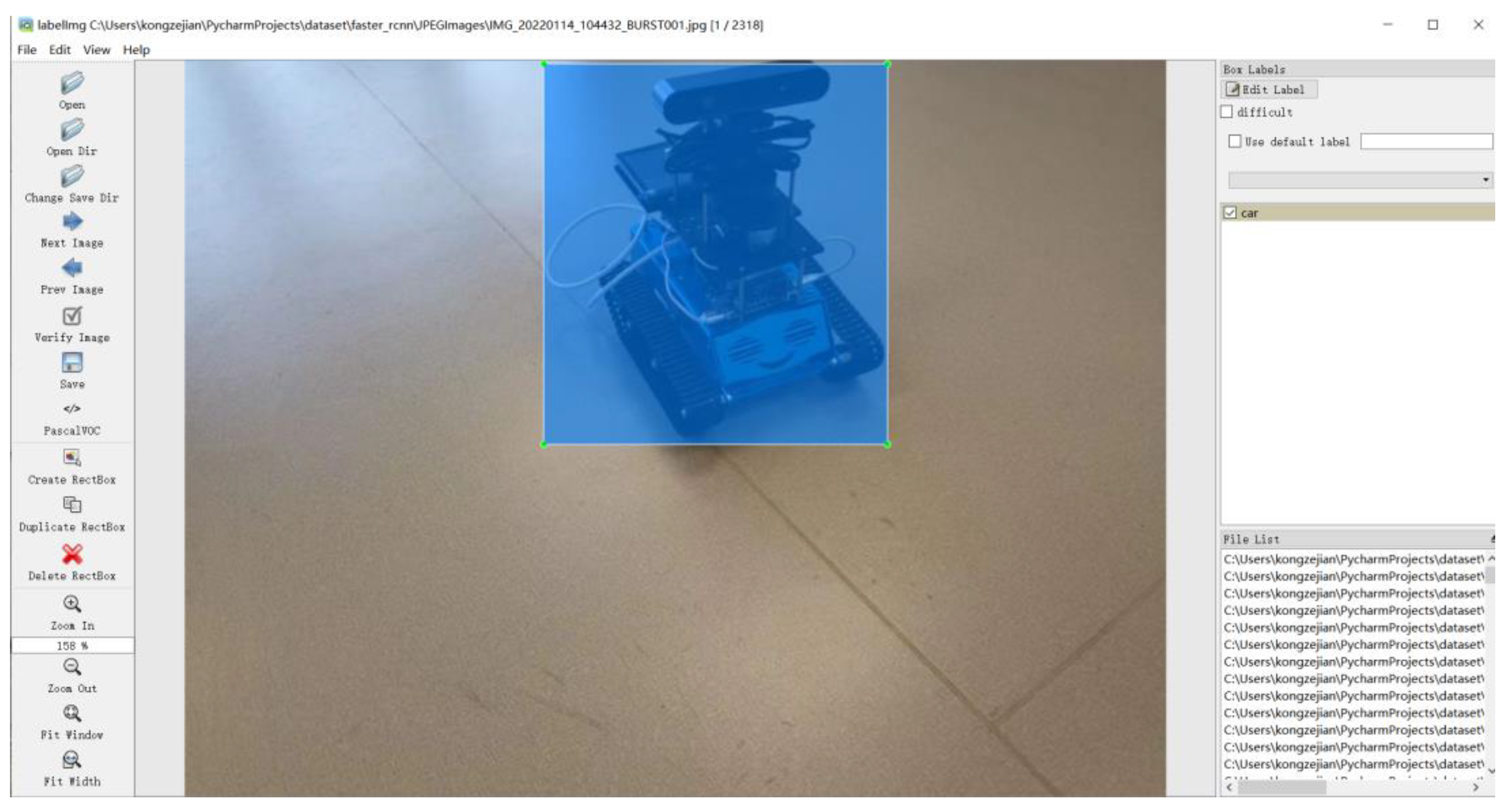
In this paper, we provide clear implementation procedures to verify the anti-occlusion performance of the three models for single target detection. Specific data sets are generated to facilitate the algorithm evaluation. The format of the data set is Visual Object Class (VOC) type. The images for training are imported to “labeling”—a deep learning annotation tool embedded in Anaconda 3. The ground truth anchors, including the classes and coordinates, are drawn manually. All images are collected from the different distances and angles of the target robot. Some images are obtained under unclear lighting and noisy conditions.
A computer program is designed to read the information of the ground truth anchors from “XML” files and generate two “txt” files for training and validation. An example can be seen in
Figure 1: Manual annotation of the object in Labeling. The graphical user interface contains three key areas which are tool bar, labeling and file list. A toolbar is located at the edge of the screen, and the image waiting to be labelled is displayed in the center of the interface. There is a file list at the low right corner edge. It illustrates the file information of the selected images.
The main parameters for the performance evaluation in the three deep learning methods include confidence, nms_iou and anchors_size. The confidence is set to 50% to balance the tradeoff and the nms_iou is set to 0.7. The setting of the anchor size is based on the traditional average value in similar cases.
Three categories of occlusion simulations are tested. One is a simulation based on data augmentation. In the second simulation, test data set two was created. The image in test data set two does not belong to the images in the target robot data set and test data set one. The targets in these images come from different angles and distances. At the same time, some targets are out of range. The occlusion is about 10% to 30% of the target. In the third simulation, we test whether these models can adapt to the change of occlusion.
3.1. Experimental Setting
The target robot data set is first created. Each image has a dimension of 4160 × 3120 pixels. All images are collected from different distances and angles of the target robot. For example, we take photos at a certain distance from the robot, and then move around to ensure that photos from different angles of the robot are collected. The distance between the robot and the camera varies under mobility. The photos are taken accordingly. The images also contain the ones taken under bad lighting conditions or noisy conditions. When the distance or angle changes, the background of the image may change as well.
The operating workspace environment includes Windows 10, CUDA 11.4, cuDNN 7.6.5, and Visual Studio 2022. The hardware used in the experiment is an NVIDIA GeForce GTX 1650 with 4096 MiB (Santa Clara, CA, USA).
The Faster RCNN, SSD and YOLOv5 models are all fast deep learning methods. To make the comparison between them as fair as possible, much attention was paid to the settings of these three models.
For the Faster RCNN model, we adopt non-maximum suppression (NMS) on the proposal regions in the RPN network and set the IoU threshold for NMS as 0.7. In the Region of Interest (ROI) pooling layer, both the numbers of the positive and negative samples are balanced to 128. Due to the different sizes of the proposed anchors, the ROI pooling obtains the output of a fixed size via the method of mapping and max pooling. For YOLOv5, there are three main steps to set up the model. First, the file train.py is called. Then in the voc_ball.yaml file, there is only one target in our experiment. The target name is called robot. The training data set and the verification data set are in the local location. Finally, settings in the yolov5s_ball.yaml file are responsible for most of the parameters. It contains a number of categories of objects in the data set, the coefficient controlling network depth, the coefficient controlling network width and the batch size. All these parameters are separately well set based on the specific experiments. For the SSD model, the steps of the matching strategy are as follows: each default anchor should be sorted according to the confidence score. The confidence threshold is set to be 0.5, which means that default anchors that have scores higher than 0.5 will be retained. After that, one object may have several default anchors, and box position and score for non-maximal suppression are used to filter anchors. The IoU for non-maximal suppression is set to 0.7. The training is divided into freeze training and unfreeze training. In freezing training, the network backbone is frozen, and more resources are used to train the posterior network parameters. For more efficient use of the GPU memory, the batch size of freeze training is 16. In the unfreeze training, the backbone network is unfrozen, and all parameters are trained at the same time. The batch size of the part is set to 4.
3.2. Data Sets
Several data sets are created. Images are collected by an 8-megapixel camera (Leica, Wetzlar, Germany) with F/2.0 aperture and a fixed focal length. All images in our data sets are collected in two environments, an indoor environment and an outdoor environment. We designed the following data sets:
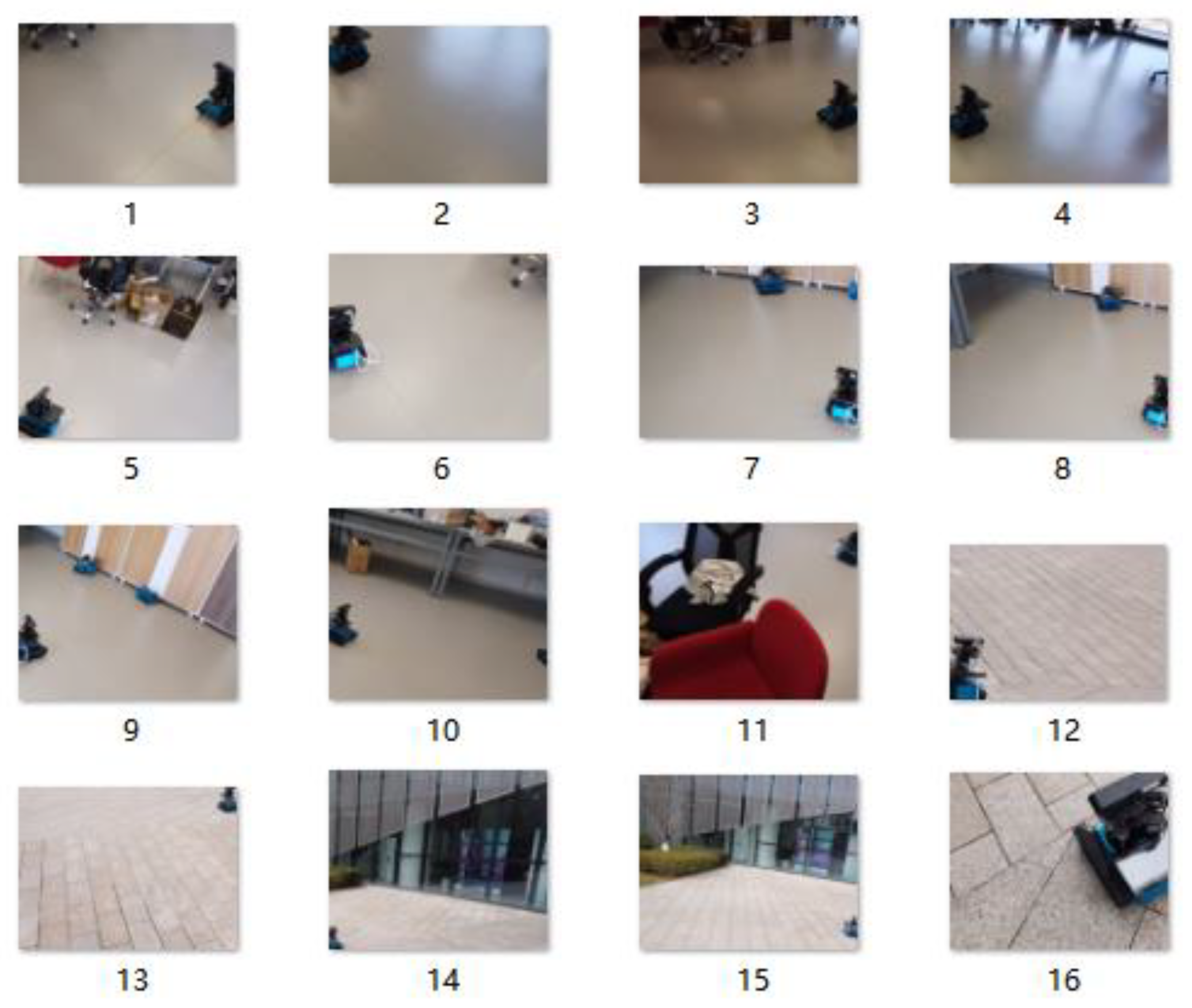
(1) A training data set. A data set containing 2993 images is created. The images are 4160 × 3120 pixels. All images have been carefully annotated and used as the training set. There is a whole target in the image. The target is captured from different distances, different angles and different circumstances. (2) Testing data set one. It contains 1718 images which are different from the training data set. All images have the same pixel as the training data set. (3) Testing data set two. The second testing data set with 661 images is also created. Images in testing data set two are chosen from the images which are not put in the target robot data set and testing data set one. The targets in these images are seen with different angles and are from different distances. Meanwhile, part of these targets is out of range. The target is missing about 10% to 30% of itself; some examples can be seen in
Figure 2: Examples of testing data set two. (4) Testing data set three. A testing data set with 599 images is created by a random erasing method.
There are some advantages to our designed data sets. First, the environments of the created data sets are different. To ensure the diversity of the environments, we take a series of actions which contain the exposure of the picture, use a random erasing method and so on. In addition, the target is captured from different distances, different angles Furthermore, some occlusion condition testing data sets are created. However, there exist some limitations of our designed data sets which should be improved in further studies. Second, the environments of the created data sets are not complicated enough. Moreover, the created data sets are relatively small. Besides, the images of the data sets keep the target from a bot close distance from the camera.
3.3. Data Augmentation
The designed program first acquires the length and width of the collected images in the data set. It then obtains the pixel points of each coordinate of the picture to facilitate the combination of pixel points. Based on the information mentioned above, the program can rearrange the pixels to create flipped images. The key point of random erasing is to select a rectangular region in an image and erase its pixels with random values [
7]. The RGB value of −3,947,833 representing grey is used for erasing. The coverage area is set as the threshold size, which can be selected according to the specific experimental needs. The test data set simulates the occlusion effect by randomly erasing the target features. It also improves the generalization ability of the model. The random erasing enables the model to recognize the target through local features in the training process. It also enhances the model cognition of the local features of the target and weakens the model’s dependence on all the features of the target. The model trained by these data is more robust to noise and occlusion. All deep learning models perform well, the random erasure method is used to create test data sets to judge the ability of these models.
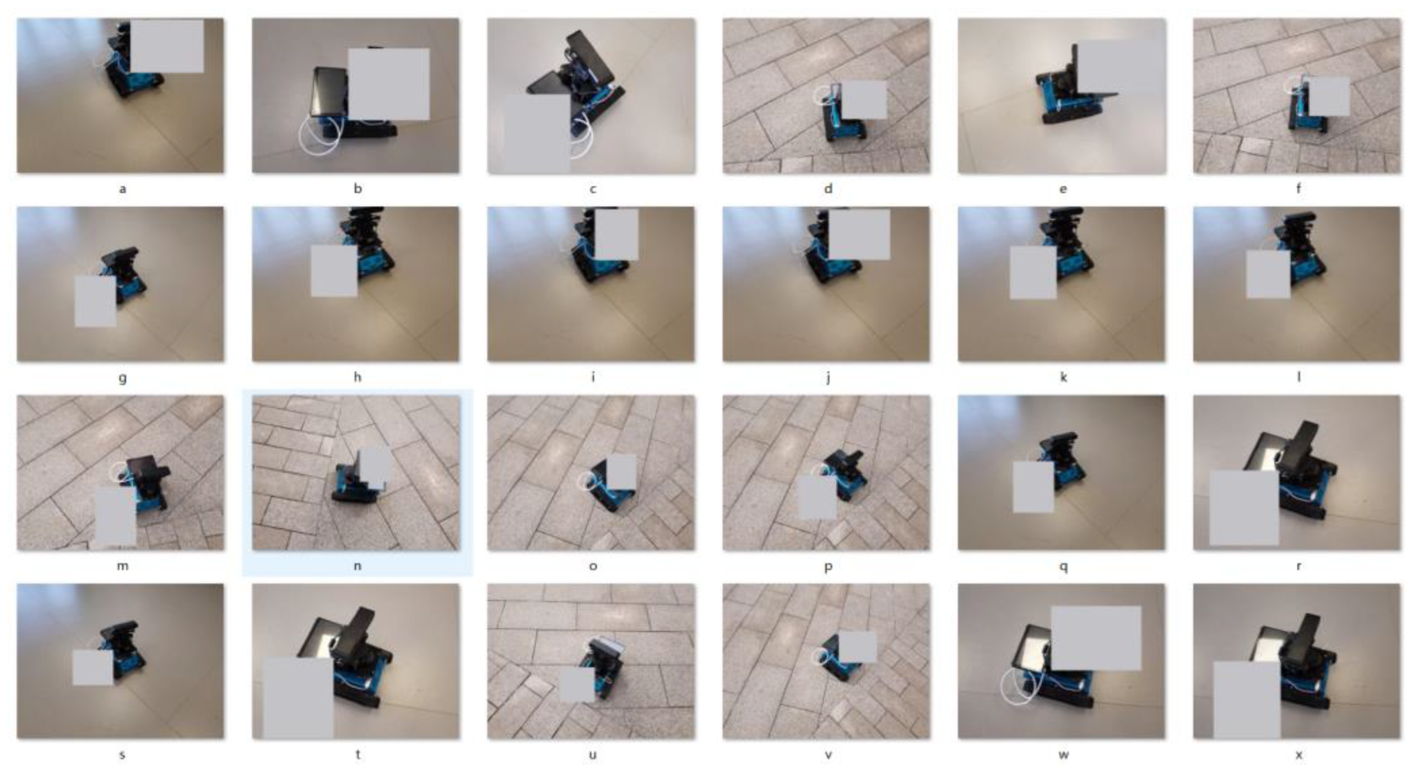
A testing data set with 599 images is constructed by a random erasing method. This set is called testing data set one and is shown in
Figure 3: Screenshot of the erased data set. These images are selected from images that have never been placed in the target robot data set. This data set depicts targets in the test set undergoing different degrees of random erasure in different environments. The data set is composed of car images in indoor and outdoor environments. These images are covered so that the light and shade change to a certain extent. Random numbers are added to enrich the data set based on the coordinate parameters selected by the label box and data enhancement operations such as erasing. We specifically designed a program to generate the test data set using this random erasure method. The area erased by the program is in accordance with the size of the target in the image. According to the label marked in the image, the program can ensure that an area of the target is identified. A starting point is then randomly created in this area. A random erasure area, which is smaller than the target area and has a random size, is generated. Therefore, all erasure areas can erase some target areas with different sizes, so as to ensure that the test data set has sufficient generalization ability.
3.4. Different Environments
The second test data set containing 661 images is created and defined as test dataset two. The images in test data set two have never been selected from the images in the target robot data set and test data set one. The targets in these images are captured from different angles and distances to simulate different mobilities. Practical occlusion is simulated for out-of-range scenarios. The images of the data set also contain images taken under harsh lighting or noisy conditions. The practical occlusion is about 10% to 30% of the target.
Furthermore, the deep learning models have different performances in detecting the object at different light intensities which can be seen in
Table 1: Testing results for deep learning models’ brightness. One image was selected from our testing data set. Then we change the exposure of the image from −5 to 5. The Faster RCNN and the SSD models can detect the object in the darkest and lightest environment. However, the Faster RCNN model produces multiple detection results for the same target. The YOLOv5 model can detect the object in the lightest environment, but it cannot detect the object in the darkest environment.
3.5. Occlusions Variation
To make a judgement on whether the SSD model, the Faster RCNN model and the YOLOv5 model are adaptive to different degrees of occlusion, we identified an image as the testing sample. The size of the image is 4160 × 3120. The upper-left and lower-left corners of the target are (1,991,811) and (2752 × 1730) respectively. We then cut the image step by step to ensure that varying occlusion of the target can be measured. The precision is controlled to the range of 1%. The experiments demonstrate that the Faster RCNN and the SSD models can handle occlusion of up to 95% under a relatively simple background. The YOLOv5 model works under up to 96% occlusion. The experiments demonstrate that the Faster RCNN can handle an occlusion of 91%. The SSD models can handle occlusion of about 80%. The YOLOv5 model works under 82.5% occlusion.
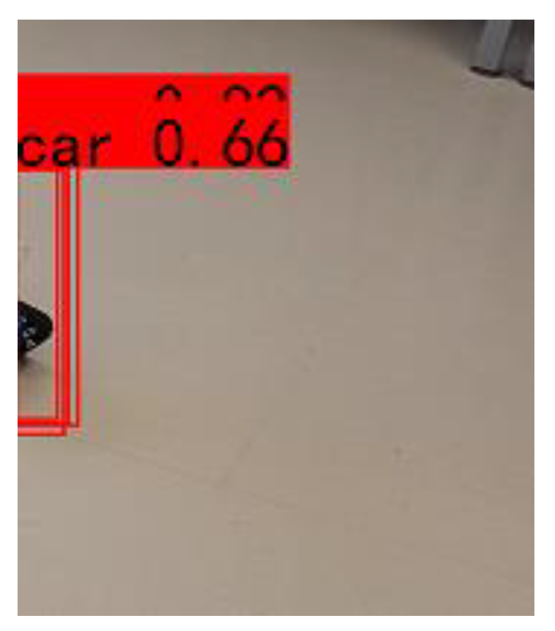
It is worth noting that the Faster RCNN model has a problematic result in the experiments. It usually marks the local features with multiple anchors on the same object during our experiments because the model is based on the candidate box extracting. This can be seen in
Figure 4: Duplicate detection in Faster R-CCN. Local features make target detection a problem for multi-scale and small targets. Multi-scale problems means that the problem studied involves multiple orders of magnitude. The feature maps extracted by Faster RCNN are all monolayers, so it is not suitable with this problem. In addition, in order to avoid re-detection, the method used by the Faster RCNN model is unfriendly to the occluded target. If the threshold is set too large, the model will result in missed detection. If the threshold is set too small, the model will re-detect. When the target only shows local features, the model will not miss detection because only a small part of the field of vision is the target. However, within this small local feature, the model will continue to subdivide, causing re-detection. For example, our data set detects one target, and the color feature is relatively simple. After the lower left corner is identified as a target, similar features inside the target will also be detected to cause re-detection for the target as shown in
Figure 4.
All three models can generally adapt well to the practical occlusion. The detection methods of these deep learning models are based on the local features of the target. Therefore, it also leads to some limitations. For example, if the training data set is not large enough, the model cannot distinguish objects of similar features from the target. However, if the training data set can provide enough possible interference and possible similar objects, the deep learning model can be more adaptive to occlusion. More details on the experiments and discussions are provided in
Section 4.
4. Results and Discussion
In this section, more numerical experimental results are presented to demonstrate the anti-occlusion performance of the deep learning models with the generated data set. YOLOv5, Faster RCNN and SSD are chosen as the benchmarks. Labeling was used to label images in the data set. The target object is the robot vehicle. After labeling the images, the model is fine-turned according to the training data set. Training time, F1 Score, Precision and Recall are adopted as evaluation metrics. Score_threshold is the threshold of confidence. Prediction results greater than this value are retained.
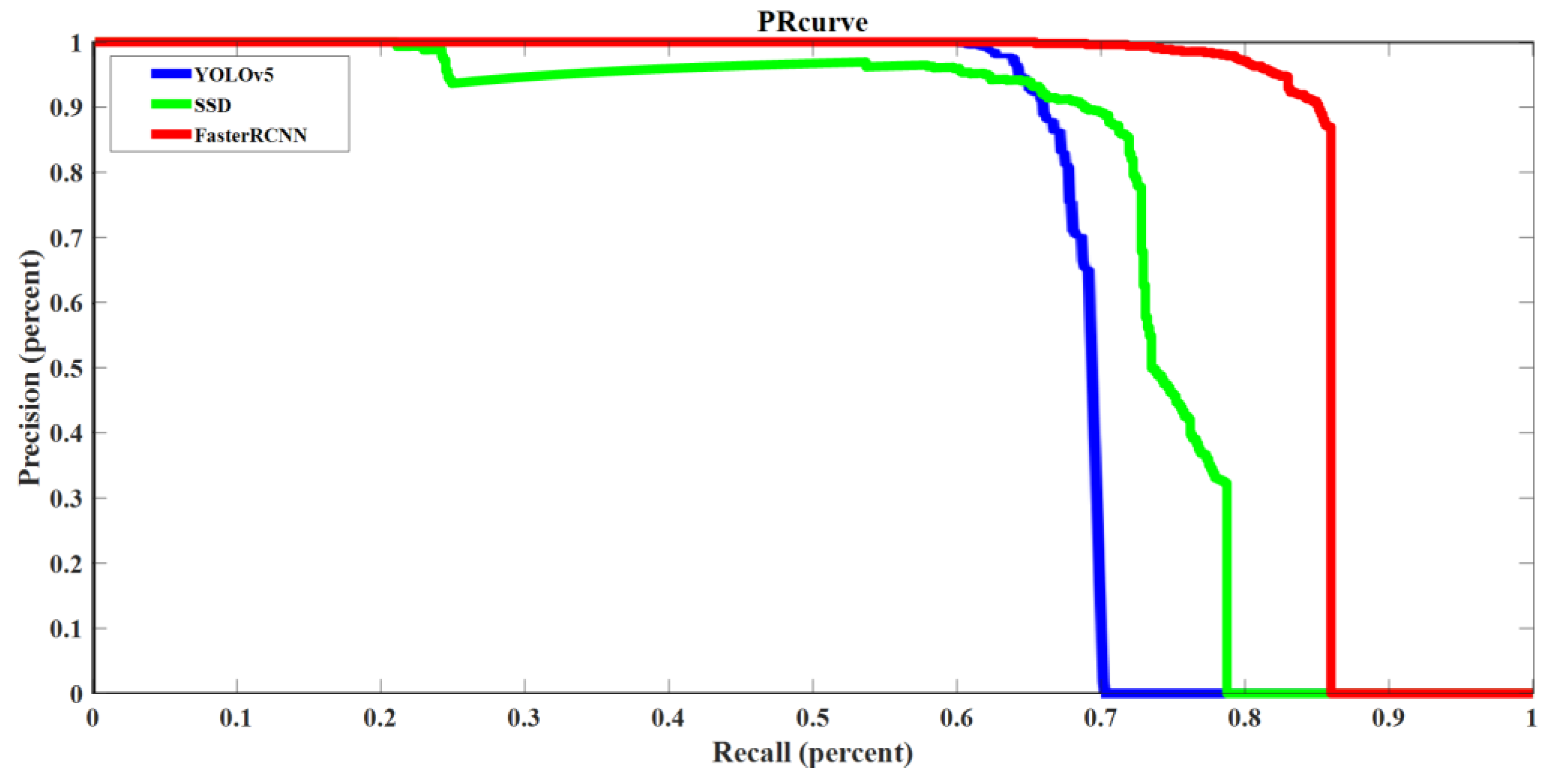
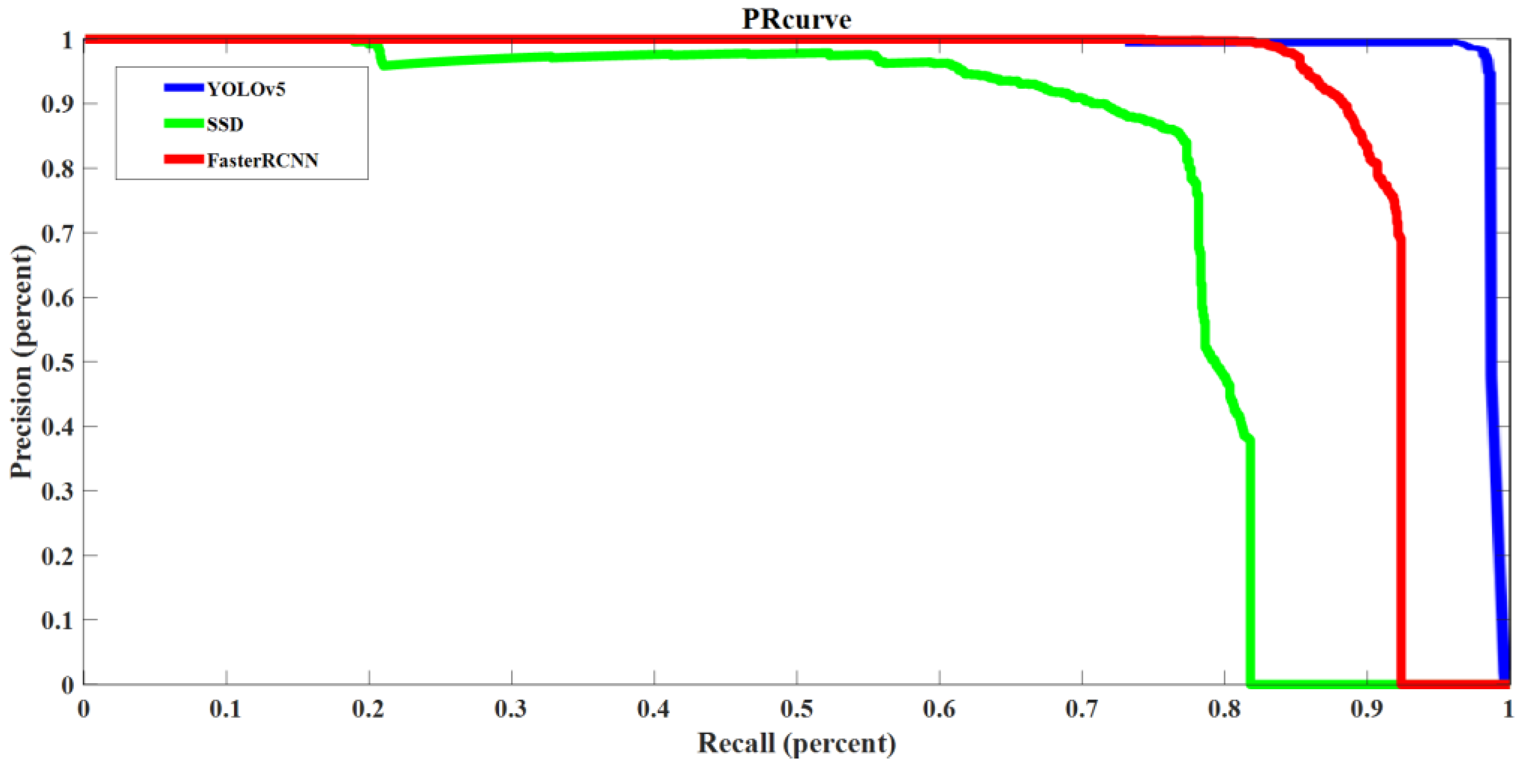
The training times of the three models are also tested. The test data set is created using the images and videos of the target robot at different angles indoors and outdoors. Initially, the random erasure method is not applied. The three models all provide perfect results with 100% accuracy and recall. When more challenging situations are simulated, i.e., when the random erasure method is adopted, the PR curves of the three models for testing data set one and testing data set two are shown in
Figure 5 and
Figure 6, respectively. As shown in
Figure 5, the Faster RCNN model has a PR curve most close to the upper right corner. The YOLOv5 has the best performance for test data two, as shown in
Figure 6. The values of precision and recall are also different under different confidence levels. The data in this project use the specified value when the confidence is set to 0.5. We need to use other testing parameters to further judge which model has the best performance.
According to
Figure 5 and
Figure 6, it is observed that the SSD model is the most stable one. For example, the Faster RCNN model reaches 0.85 recall in
Figure 5 and 0.92 recall in
Figure 6 when the precision is 0. The YOLOv5 model reaches 0.7 recall in
Figure 5 and 1 recall in
Figure 6 when the precision is 0. The SSD model maintains about 0.8 recall in
Figure 5 and
Figure 6 when the precision is 0. Therefore, the SSD model is the most stable model when dealing with different testing data sets. The reason is that the size and position of the prior frame of SSD are set in advance, which makes it simple and is less affected by the environment.
The configuration files of the models are also modified to train the data set. Accuracy quantifies the correlation of detection targets. Recall refers to the ratio of detected targets to all existing targets. The F1 score is an index used to measure the accuracy of the binary classification model in statistics. It takes into account the accuracy and recall of the classification model. The training time of these models is also tested.
As shown in
Table 2: Testing Results for testing data set one, Faster RCNN and SSD have a comparable performance of 0.87 and 0.89 respectively in the F1 score, which is much better than 0.54 with the YOLOv5 model. The SSD model achieves the highest F1 score. The precision of Faster RCNN, SSD and YOLOv5 are 93.38%, 97.72% and 97.69%. The SSD model achieves the highest precision value. The recall values of Faster RCNN, SSD and YOLOv5 are 77.62%, 81.16% and 63.66%, respectively. Again, the SSD model achieves the highest value. As shown in
Table 3: Testing Results for testing data set two, the F1 score for three models are 0.89, 0.81 and 0.98. The Faster RCNN model achieves the highest F1 score. The precision of Faster RCNN, SSD and YOLOv5 is 91.55%, 76.96% and 98.18%. The YOLOv5 model achieves the highest precision value. YOLOv5 also achieves a high score of 98.18% for the recall, which is better than the recall scores of 87.54% and 81.99% for Faster RCNN and SSD, respectively. Meanwhile, the Faster RCNN model spends about 48.25 h on training. The SSD model spends the least training time, about 15.16 h. The YOLOv5 model spends about 20.25 h on training. The detection speed of Faster RCNN is about 1.6 frames per second. For SSD and YOLOv5 models, the detection speeds are about 6.6 and 3 frames per second, respectively.
According to the values in
Table 2: Testing Results for testing data set one and
Table 3: Testing Results for testing data set two, it is difficult to decide which model has the best overall performance. In order to further judge the performance of these models, we defined a variable called
P which stands for the performance of the model in the designed experiments. The F1 score is regarded as an index to measure the accuracy of the binary classification model in statistics. It takes into account both the accuracy and recall of the classification model. F1 score can be regarded as the weighted average of model accuracy and recall rate. Its maximum value is 1 and its minimum value is 0. In general, the larger the F1 score is, the better the model’s performance. The training time is the time spent by the model to train the data set. The detection speed is how many frames the model can detect per second. As the values of the F1 score and the detection speed should be as high as possible and the value of the training time should be as low as possible, the performance of the model can be determined accordingly. The function of
P can be formulated as follows:
The higher the value of
P, the better the model performance will be. Based on
Table 2, it can be calculated that
,
and
. Based on
Table 3, the three values can be derived as
,
and
. According to the results, it can be concluded that the SSD model has the best performance.
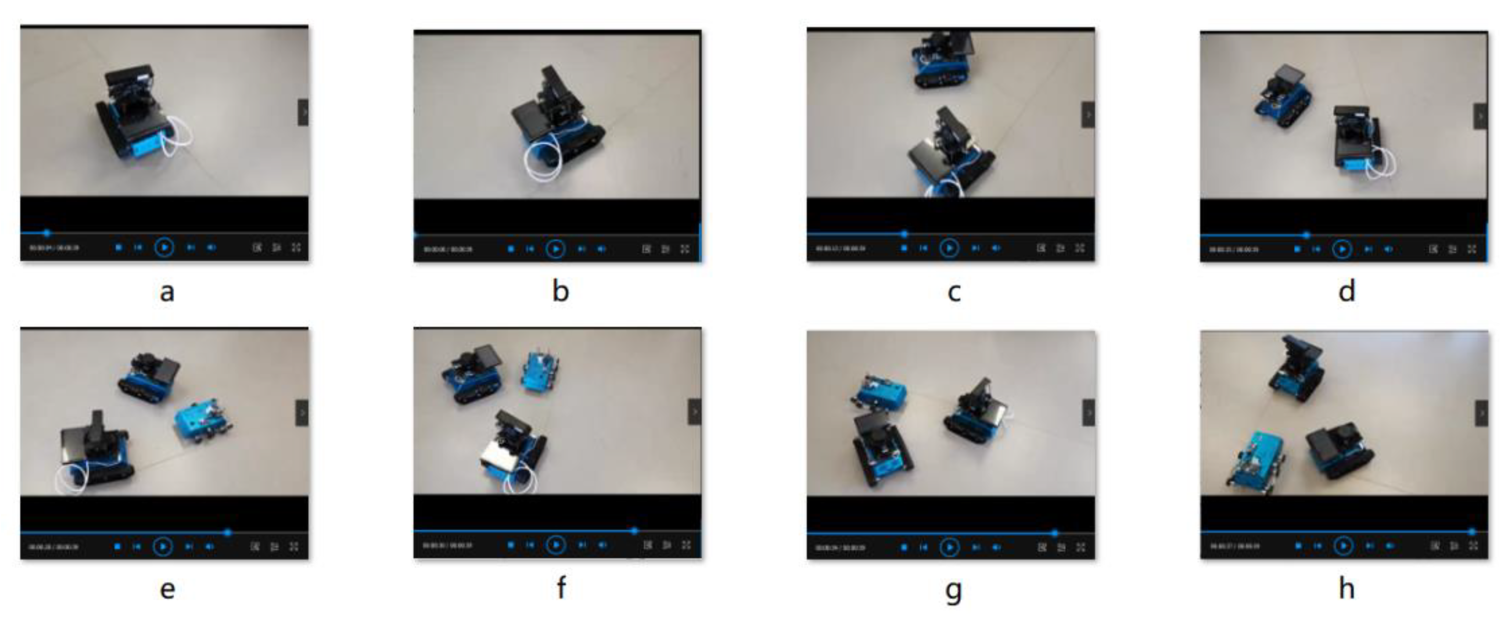
For further analysis of whether classic deep learning model tracking methods can adapt to various occlusion conditions and to what extent occlusion could be handled in a specific environment, a video containing our target and two similar objects was created to test the performance of the Faster RCNN model, SDD model and YOLOv5 model. This is a thirty-nine second-long video with thirty frames per second. An example of the video can be seen in
Figure 7: Screenshot of the testing video. At first, the target is located on the screen as shown in
Figure 7a,b. Then, a similar object is placed in the screen as shown in
Figure 7c,d. After that, a third similar object is placed on the screen, as shown in
Figure 7e. While filming the target, the photographer constantly changes the angles and keeps a relatively close distance to the target which can be seen in
Figure 7f–h.
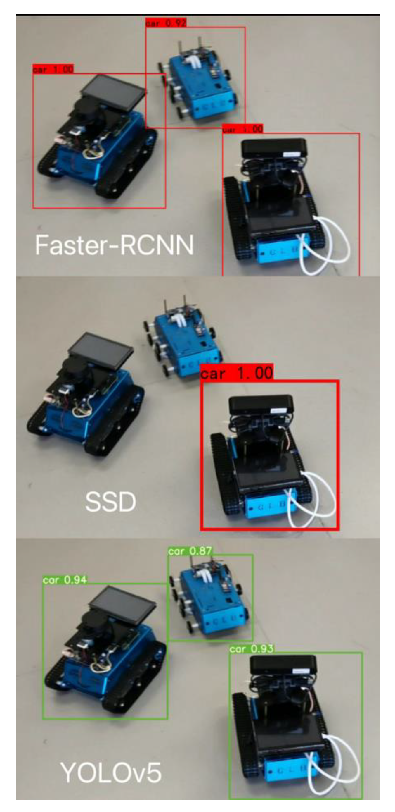
The testing results can be seen in
Figure 8: Three models’ testing results in the same frame.
In
Figure 8, the object in the lower right corner is the target. The other two objects are interferents.
Figure 8 shows that in the same frame, the Faster RCNN model detected the target, but also incorrectly identified the similar objects. The SSD model successfully detected the target and ignored the similar objects. The YOLOv5 model detected the target, but incorrectly identified the similar objects and gave one of the similar objects a higher possibility than the true target.
Based on the results, it can be concluded that the SSD model has the best performance in the designed experiments. The SSD model has the lowest training time, the highest F1 score, the highest precision, the highest recall and the fastest detection speed. The SSD model achieves the highest performance score in two testing data sets. Such experiments and dataset design methods can be applied to other specific circumstances. However, the some limitations still exist in the experiments. First, the environments of the created data sets are not complicated enough. Second, the created data sets are relatively small. Third, the images of the data sets keep the target from a bot with a close distance from the camera. Those limitations should be improved in further research.
5. Conclusions
This paper provided a comparative study of Faster RCNN, SSD and YOLOv5 for mobile robot tracking. All three deep learning models are adaptive to partial occlusion of different degrees as analyzed. We apply these models to specific experiments including erased situations, darkest environment, brightest environment, clear environment, complex environment and variation of occlusions. The performance of the models was demonstrated in terms of F1 score, precision, recall, floating points of operations and training time. A variable P was created to compare the performance of the models. Four high-quality data sets were generated to facilitate the performance evaluation. The random erasing method and occlusion from different angles were applied to augment the data sets covering various scenarios of partial occlusion.
Experimental results showed that the SSD model has the best performance and is most promising for the addressed application. The P score of the SSD model achieved 0.387 in the first testing experiment which is higher than the Faster RCNN method by about 14 times. The P score of SSD was higher than the YOLO model by about four-fold in the first testing experiment. In the second testing experiment, the P score of SSD also had a consistent performance. It achieved a score of 0.353, which is higher than the Faster RCNN by about 12 times. It was also higher than the YOLOv5 model by about threefold.
The analysis revealed different features of the implementation of the three models. The performance of the models differs in terms of the anti-interference ability, detection speed and the ability to determine the object according to the detection of local features. The analysis results may serve as a reference for the model selection to meet specific design metrics. There is also much room for improvement with the current algorithm design and performance evaluation. For example, the images of the current robot data set contain a single robot target. Further tests can be carried out to include more robots in the scene.
In the future work, we will improve our data sets. The size of current data sets is small and the diversity of the backgrounds should be expanded. The performance of the current deep learning algorithms is not satisfactory in the detection of small objects. To address the issue, the deeper layers and shallower layers can be concatenated to enrich the semantic information of the shallower layers. In addition, some deep learning models have the structure of a single stage. They can be developed into a multi-stage solution which can increase the precision of detection and localization of small objects.


 ,
, 


