In-Structure Response Spectra of an Auxiliary Building in a Nuclear Power Plant Considering Equipment–Structure Interaction

Abstract

A two-degree-of-freedom (two-DOF) equation of motion was derived in the frequency domain using a substructuring technique for efficiently calculating the in-structure response spectrum (ISRS) considering equipment–structure interaction. The model of the primary structure was condensed into a mechanical impedance function and combined with the equipment represented by a single-degree-of-freedom oscillator in the frequency domain. This condensed two-DOF system is applied to the efficient calculation of the ISRS considering the equipment–structure interaction without repeated analysis of the coupled model with full DOFs. This coupled analysis procedure was applied to a finite element model of an auxiliary building in a nuclear power plant to validate both the accuracy and impact on the equipment response. Finally, the adequacy of three representative decoupling criteria on the necessity of coupled analysis was investigated by applying those criteria to the auxiliary building example.

1. Introduction

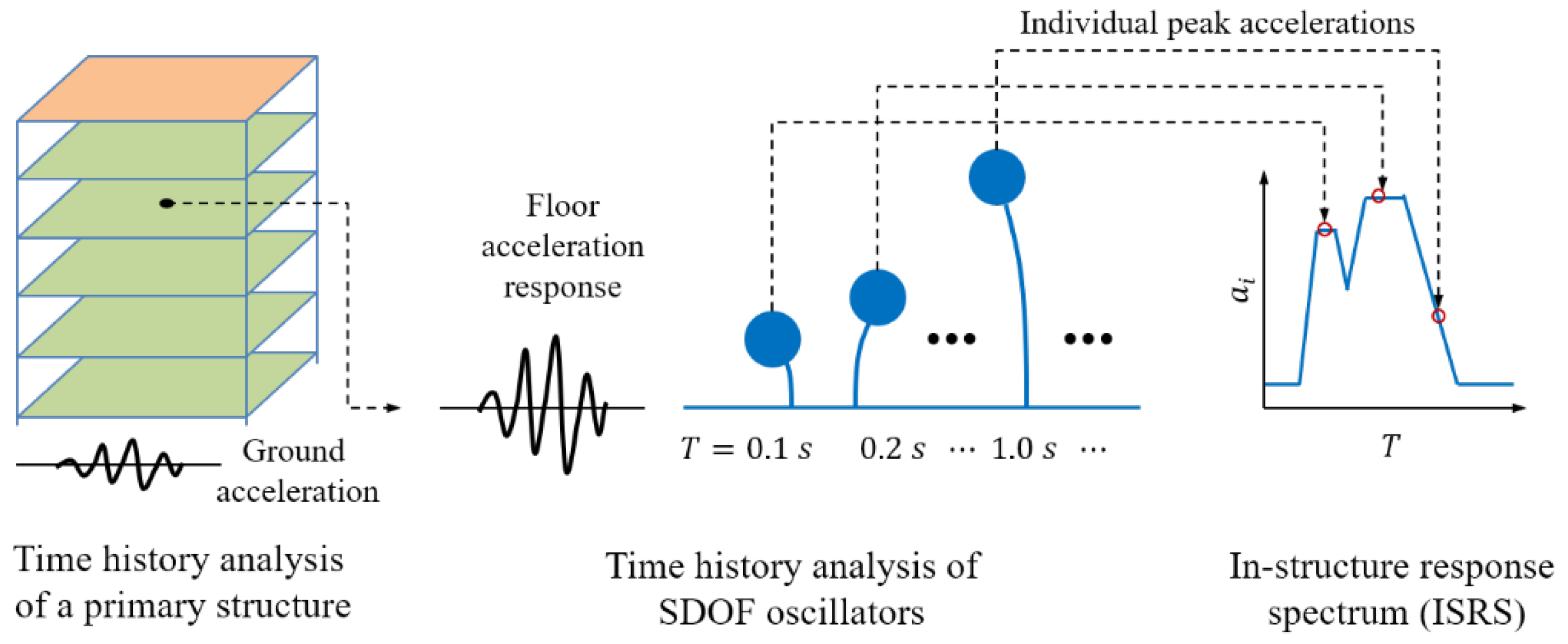
In nuclear power plants (NPPs), a primary system, usually a building or non-building structure, and many secondary systems, usually composed of equipment, are connected to each other. In the design or seismic fragility assessment of equipment installed in a structure, an in-structure response spectrum (ISRS) is used as the input motion for the equipment. The ISRS represents the peak acceleration response of a single-degree-of-freedom oscillator located in a structure excited by ground motions. The ISRS is computed for different natural frequencies of the oscillator and plotted in the form of acceleration versus natural frequency. The procedure for calculating ISRS is presented in Figure 1. The ISRS is important in the safety evaluation of equipment located in an NPP structure because various equipment has different natural frequencies and the uncertainty in natural frequency is necessary to be considered in the probabilistic safety assessment [1].

The ISRS is usually computed based on the response acceleration at individual equipment locations obtained using a structural model decoupled from the equipment. Relatively heavy equipment was considered in the analysis by adding only the mass of the equipment to the structural model. However, the ISRS computed based on decoupled analysis may have excessive conservatism compared with coupled analysis, particularly when the equipment and structure interact in resonance [2]. Therefore, excessive conservatism in the ISRS by decoupled analysis leads to a conservative design of the equipment, which increases rigidity and causes more frequent vibrations, making the components of the equipment more vulnerable to fatigue failure [3]. In addition, the ISRS obtained from the decoupled analysis has a limitation in that it can yield inaccurate equipment responses that may be non-conservative [4]. ASCE/SEI 4–16, which addresses the seismic analysis of NPPs, requires a coupled analysis when the structural response differs by more than 10% and provides graphical criteria based on the mass and frequency ratios between the primary and secondary systems to determine whether a coupled analysis is required [5]. The USNRC allows decoupled analysis under several conditions, such as highly flexible support connecting the structure and equipment [6]. Apart from the dynamic characteristics of the primary structure, soil parameter uncertainty may influence significantly the ISRS [7]. In the case of more general building structures, the influence of the inelastic structural behavior on the ISRS was investigated [8].

To obtain the ISRS through flexible analysis, it is necessary to analyze many coupled systems, each comprising the same primary system and a single degree of freedom (SDOF) oscillator representing the secondary system. The natural frequency of the oscillator differs for each coupled system and corresponds to the frequency in the abscissa of the ISRS. The fundamental methodology of the coupled analysis considering the equipment–structure interaction was established in the past. Gupta (1996), and Gupta and Gupta (1995) proposed an analytical method for transforming the eigenvalues and eigenvectors of multi-degree-of-freedom (MDOF) subsystems to obtain the modal characteristics of the coupled system [3,4]. Jiang et al. (2015) and Li et al. (2015), Wang et al. (2022) developed and validated a direct-spectra-to-spectra method to compute the ISRS directly from the response spectrum of the ground motion based on the modal combination of the coupled system [9,10,11]. These methods have the disadvantage of being limited to modal analysis. As the modal characteristics of the coupled system change whenever the natural frequency of the secondary system change, the response of the entire system must be recalculated correspondingly. On the other hand, Tseng (1989) derived a transfer function between the acceleration response of the decoupled primary structure and that of the secondary system comprising a coupled system [12]. Choi and Lee (2005) validated Tseng’s method by comparison with the coupled analysis result for an NPP containment building connected to an SDOF oscillator [13]. Tseng’s method was derived by serially connecting the dynamic stiffnesses of the primary structure and the secondary system, but the acceleration response of the decoupled primary structure is not applied to the connection between the secondary and primary systems but to the boundary between the primary system and ground. So, the analytical model is difficult to explain physically.

Recently, the interaction impact on the response of equipment in NPPs has been investigated. It was reported that the ISRS computed through decoupled analysis significantly increased in the proximity of the dominant natural frequency of the primary structure, a containment building in this case, compared to the coupled analysis [13]. Perez et al. (2015) computed ISRSs at different locations of a reinforced concrete building using a finite element (FE) model and investigated the difference between the ISRSs computed by coupled and decoupled analysis, respectively [2]. Cho and Gupta (2020) applied the methodology of Gupta (1995) to the lumped mass stick (LMS) model of an NPP structure to investigate the reduction of the ISRS by coupled analysis [3,14]. Kwag et al. (2022) build a coupled analysis model based on the LMS model of an NPP containment building and investigated response reduction effects obtained by coupled analysis [15]. Jayarajan compared the responses of coupled and decoupled analyses for petrochemical facilities [16]. Dubey et al. (2019) investigated the response reduction effect of coupled analysis at various locations and equipment masses in an NPP auxiliary building using a three-dimensional FE model [17]. In EPRI 3002009429, Tseng’s coupled analysis method using transfer functions was applied to an idealized structure in which only slabs have flexibility while the other components are rigid [18]. The coupled analysis effect was greater in the vertical direction than in the horizontal direction because the mass ratio of the equipment to the modal mass was large in the local vibration mode of the slabs. Model fidelity makes difference in the accuracy of ISRS [19]. Some researchers utilized shaking table test results to validate model adequacy and ISRS. Jha et al. (2017) investigated the influence of inelastic deformation on the ISRS and showed that an equivalent linear model of a shaking table test specimen produced an ISRS matching test results [20]. Rahman et al. (2022) investigated the influence of location on the floor response using a three-dimensional FE model updated to fit the shaking table test result of a reinforced concrete building specimen [21]. Although they considered equipment-structure interaction in the analysis, their approach was based on the repeated analysis of a model with entire DOFs.

In this study, a two-degree-of-freedom (two-DOF) equation of motion was derived in the frequency domain using a substructuring technique for efficiently calculating ISRS considering the equipment–structure interaction. The ISRS of the auxiliary building was efficiently calculated using only a single calculation of the impedance function and structural response conducted for the decoupled primary system. Repeated analyses of the coupled model for different equipment frequencies were conducted using the model with only two DOFs, instead of analyzing the coupled model with full DOFs. Compared to the transfer function method, the proposed two-DOF model enables clear physical interpretation and computes the response of the primary structure at once in addition to the secondary system response.

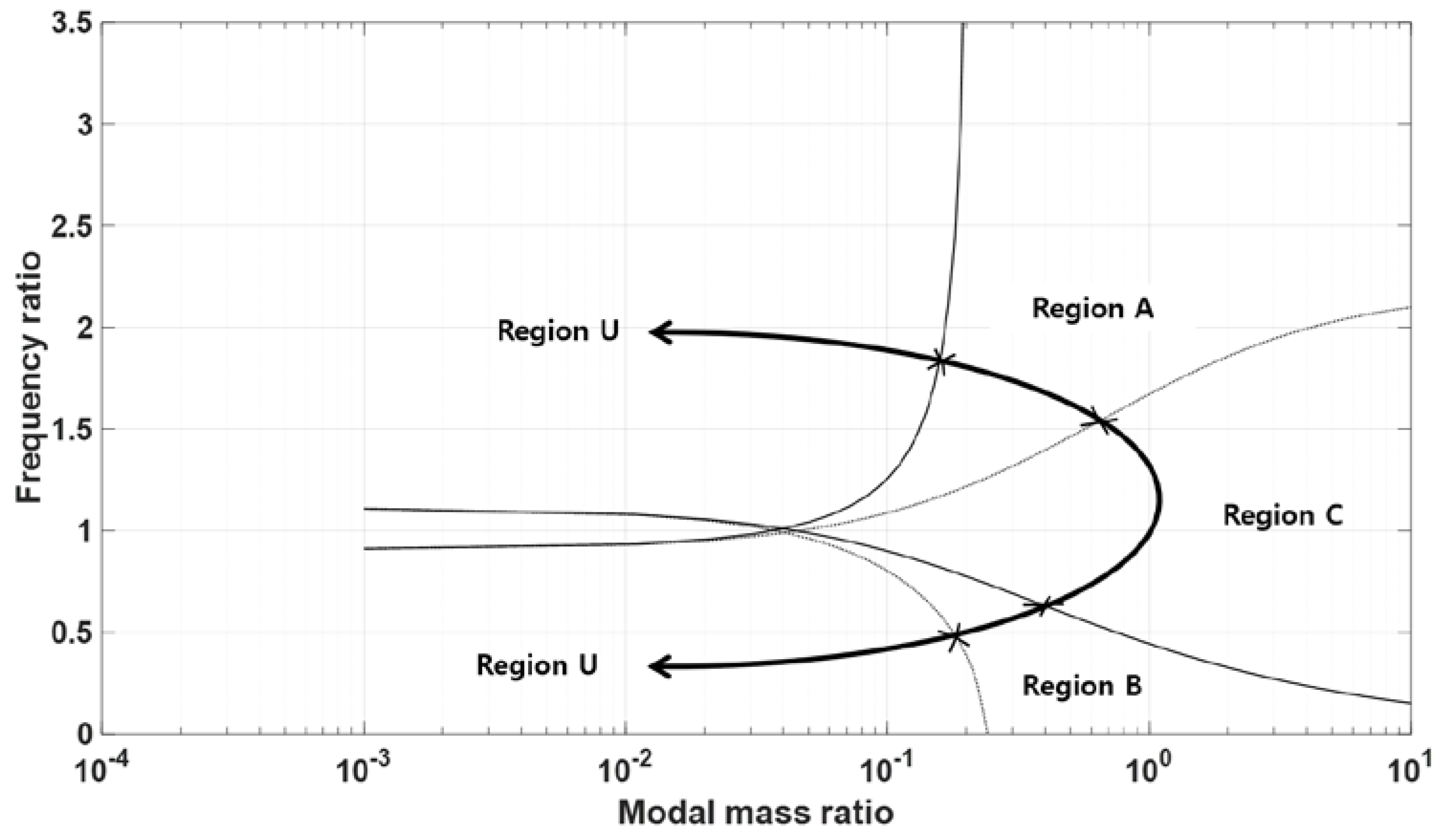
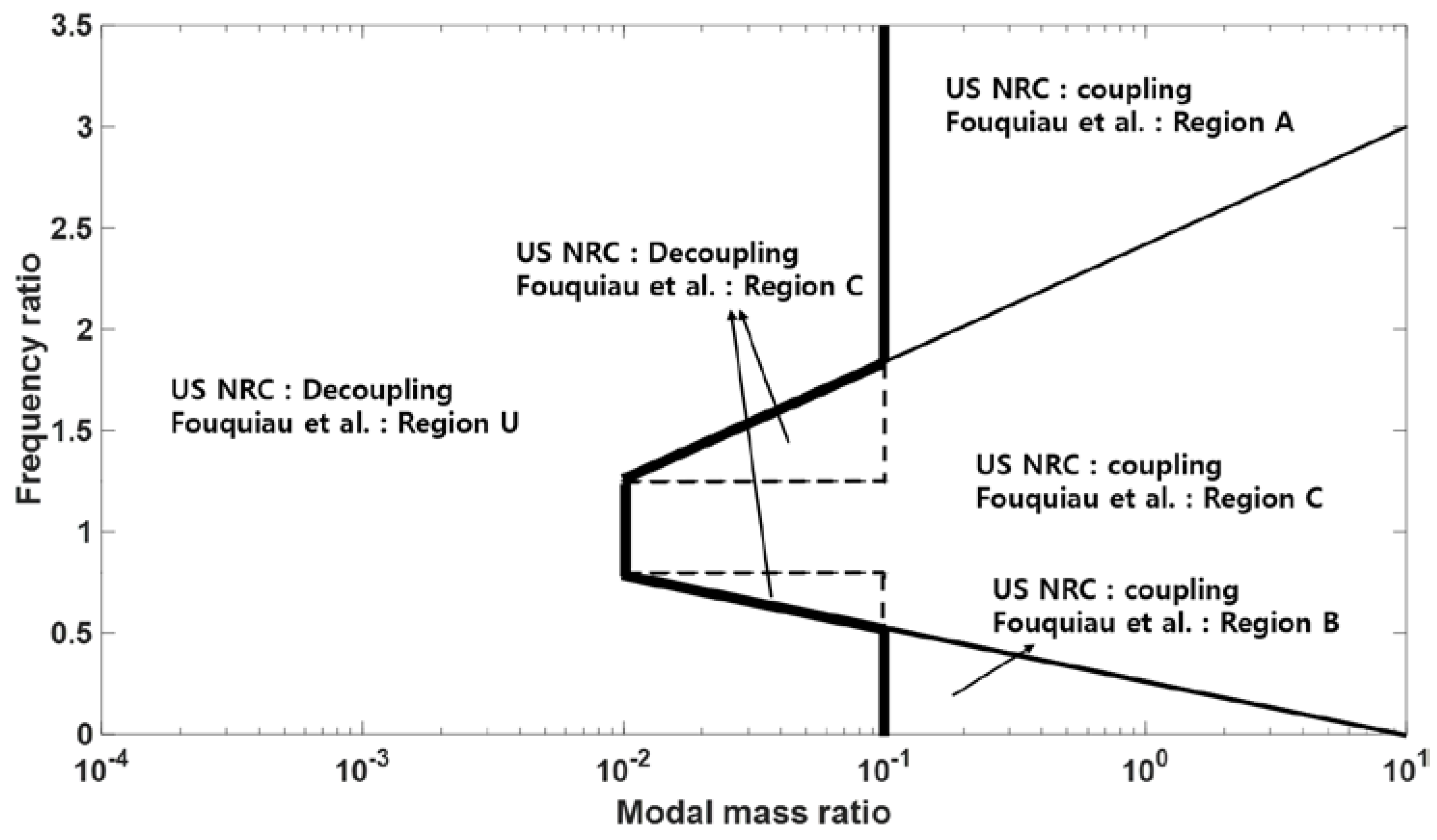
Apart from the coupled analysis technique, decoupling criteria is another important issue in equipment-structure interaction. Therefore, the adequacy of the three decoupling criteria was investigated in this study. Two representative decoupling criteria adopted in ASCE/SEI 4–16 and NUREG-75/087, respectively, were applied to the design of NPP and the other criteria recently developed by Fouquiau et al. (2018) were adopted in this study [5,22,23]. All the criteria were developed based on the simplified coupled systems of which both primary system and secondary systems are modeled with SDOF systems. However, the validation of those criteria using complex NPP structures is hard to find. A recent study by Jung et al. (2020) investigated all three criteria but their study was limited to simple systems with only a single DOF [24]. This study investigated the adequacy of those three decoupling criteria using an auxiliary building model and the proposed coupled analysis technique and proposed improved criteria by combining two of those.

In Section 2, the coupled analysis method using the two-DOF equation of motion is presented in the frequency domain. In Section 3, the FE model of an auxiliary building in an NPP is built using commercial FE analysis software for validating the proposed method to calculate ISRS and investigating the equipment–structure interaction effect on the ISRS of NPP structures with a large mass. In Section 4, ground motions applied to the numerical analysis are described in detail. In Section 5, the ISRS obtained using the proposed coupled analysis method and the analysis using the coupled model with full DOFs were compared for verification. The impact of the equipment–structure interaction on the ISRS was investigated through a parametric study, in which the location of the equipment, the direction of the equipment motion, the mass ratio between the equipment and building structure, the damping ratio of the equipment, and stiffness change due to cracking were considered. Finally, in Section 6, the adequacy of the three representative criteria using the modal mass ratio and frequency ratio to determine the necessity of coupled analysis was investigated by applying the criteria to the example auxiliary building and combined criteria are proposed.

2. Equation of Motion for a Structure Coupled with an Equipment

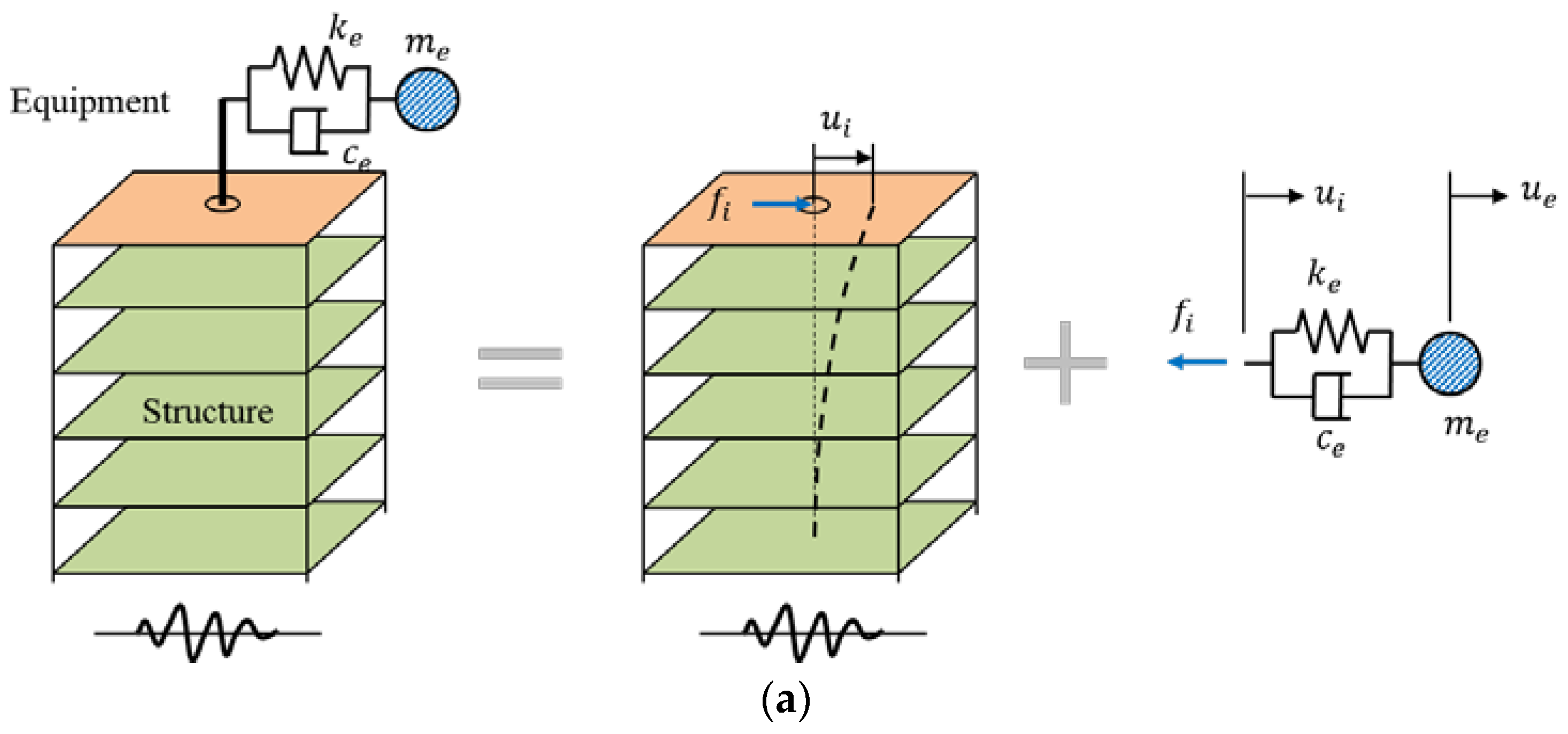
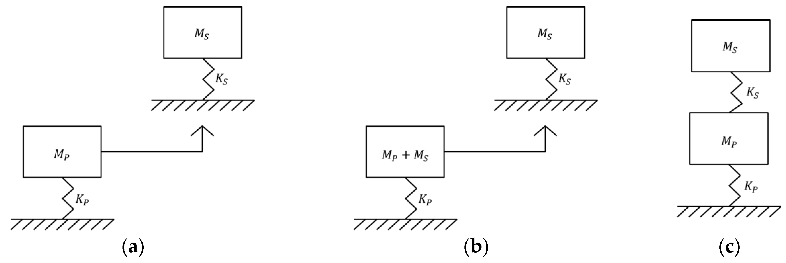
The equations of motion for a structure coupled with equipment are formulated assuming that the primary system is an MDOF structure, and the equipment is represented by an SDOF oscillator, as shown in Figure 2a. The equations of motion for the equipment and structure are expressed by Equations (1) and (2), respectively, as follows:

$$\left[\begin{array}{cc}0& 0\\ 0& m_e\end{array}\right]\left\{\begin{array}{c}{\ddot{u}}_i\\ {\ddot{u}}_e\end{array}\right\}+\left[\begin{array}{cc}{c}_e& -c_e\\ -c_e& c_e\end{array}\right]\left\{\begin{array}{c}{\dot{u}}_i\\ {\dot{u}}_e\end{array}\right\}+\left[\begin{array}{cc}{k}_e& -k_e\\ -k_e& k_e\end{array}\right]\left\{\begin{array}{c}{u}_i\\ u_e\end{array}\right\}=-\left\{\begin{array}{c}0\\ m_e\end{array}\right\}{\ddot{u}}_g-\left\{\begin{array}{c}{f}_i\\ 0\end{array}\right\}$$

(1)

$$\left[\begin{array}{cc}{\mathit{m}}_{\mathit{s}\mathit{s}}& \mathbf{0}\\ {\mathbf{0}}^T& m_{ii}\end{array}\right]\left\{\begin{array}{c}{\ddot{\mathit{u}}}_s\\ {\ddot{u}}_i\end{array}\right\}+\left[\begin{array}{cc}{\mathit{c}}_{\mathit{s}\mathit{s}}& -{\mathit{c}}_{\mathit{s}\mathit{i}}\\ -{\mathit{c}}_{\mathit{i}\mathit{s}}& c_{ii}\end{array}\right]\left\{\begin{array}{c}{\dot{\mathit{u}}}_{\mathit{s}}\\ {\dot{u}}_i\end{array}\right\}+\left[\begin{array}{cc}{\mathit{k}}_{\mathit{s}\mathit{s}}& -{\mathit{k}}_{\mathit{s}\mathit{i}}\\ -{\mathit{k}}_{\mathit{i}\mathit{s}}& k_{ii}\end{array}\right]\left\{\begin{array}{c}{\mathit{u}}_s\\ u_i\end{array}\right\}=-\left\{\begin{array}{c}{\mathit{m}}_{\mathit{s}}{\mathit{l}}_{\mathit{s}}\\ m_{ii}\end{array}\right\}{\ddot{u}}_g+\left\{\begin{array}{c}0\\ f_i\end{array}\right\}$$

(2)

where $u_i$ is the displacement at the interface between the equipment and structure; $u_e$, ${\mathit{u}}_{\mathit{s}}, f_i$ and ${\ddot{u}}_g$ are the displacements of the equipment and structure, interaction force between the equipment and structure, and ground acceleration, respectively. In addition, ${\mathit{m}}_{\mathit{e}}$, ${\mathit{c}}_{\mathit{e}}$ and ${\mathit{k}}_{\mathit{e}}$ are the mass, damping coefficient, and stiffness of the equipment, respectively; ${\mathit{m}}_{\mathit{s}\mathit{s}}$, and $m_{ii}$ are the mass of the structure; ${\mathit{c}}_{\mathit{s}\mathit{s}}$, ${\mathit{c}}_{\mathit{s}\mathit{i}}$, ${\mathit{c}}_{\mathit{i}\mathit{s}}$ and $c_{ii}$ are the damping of the structure; ${\mathit{k}}_{\mathit{s}\mathit{s}}$, ${\mathit{k}}_{\mathit{s}\mathit{i}}$, ${\mathit{k}}_{\mathit{i}\mathit{s}}$ and $k_{ii}$ are the stiffness of the structure; and the subscripts $i$ and $s$ indicate the DOFs at the interface of the equipment and the structure, and the other DOFs in the structure, respectively.

Equations (1) and (2) can be transformed into Equations (3) and (4), which are defined in the frequency domain using Fourier transform.

$$\left(\left[\begin{array}{cc}{k}_e& -k_e\\ -k_e& k_e\end{array}\right]-{\omega }^2\left[\begin{array}{cc}0& 0\\ 0& m_e\end{array}\right]+j\omega \left[\begin{array}{cc}{c}_e& -c_e\\ -c_e& c_e\end{array}\right]\right)\left\{\begin{array}{c}{U}_i\\ U_e\end{array}\right\}=-\left\{\begin{array}{c}0\\ m_e\end{array}\right\}{\ddot{U}}_g-\left\{\begin{array}{c}{F}_i\\ 0\end{array}\right\}$$

(3)

$$\left(\left[\begin{array}{cc}{\mathit{k}}_{\mathit{s}\mathit{s}}& -{\mathit{k}}_{\mathit{s}\mathit{i}}\\ -{\mathit{k}}_{\mathit{i}\mathit{s}}& k_{ii}\end{array}\right]-{\omega }^2\left[\begin{array}{cc}{\mathit{m}}_{\mathit{s}\mathit{s}}& \mathbf{0}\\ {\mathbf{0}}^T& m_{ii}\end{array}\right]+j\omega \left[\begin{array}{cc}{\mathit{c}}_{\mathit{s}\mathit{s}}& -{\mathit{c}}_{\mathit{s}\mathit{i}}\\ -{\mathit{c}}_{\mathit{i}\mathit{s}}& c_{ii}\end{array}\right]\right)\left\{\begin{array}{c}{\mathit{U}}_{\mathit{s}}\\ U_i\end{array}\right\}=-\left\{\begin{array}{c}{\mathit{m}}_{\mathit{s}}{\mathit{l}}_{\mathit{s}}\\ m_{ii}\end{array}\right\}{\ddot{U}}_g+\left\{\begin{array}{c}0\\ F_i\end{array}\right\}$$

(4)

where $\omega$ is the circular frequency; $j$ is the imaginary number; and $U_e$, $U_i, {\mathit{U}}_s, {\ddot{U}}_g$ and $F_i$ are the Fourier transforms of $u_i$, $u_e$, ${\mathit{u}}_s$, ${\ddot{u}}_g$ and $f_i$, respectively. The frequency-dependent dynamic characteristics of the equipment and structure are combined with the dynamic stiffnesses corresponding to each DOFs so that Equations (3) and (4) are rewritten as follows:

$$\left[\begin{array}{cc}{K}_{ii}& K_{ie}\\ K_{ei}& K_{ee}\end{array}\right]\left\{\begin{array}{c}{U}_i\\ U_e\end{array}\right\}=-\left\{\begin{array}{c}{F}_i\\ m_e{\ddot{U}}_g\end{array}\right\}$$

(5)

$$\left[\begin{array}{cc}{\mathit{K}}_{\mathit{s}\mathit{s}}& {\mathit{K}}_{\mathit{s}\mathit{i}}\\ {\mathit{K}}_{\mathit{i}\mathit{s}}& K_{ii}\end{array}\right]\left\{\begin{array}{c}{\mathit{U}}_{\mathit{s}}\\ U_i\end{array}\right\}=-\left\{\begin{array}{c}{\mathit{m}}_{\mathit{s}}{\mathit{l}}_{\mathit{s}}{\ddot{U}}_g\\ m_{ii}{\ddot{U}}_g-F_i\end{array}\right\}$$

(6)

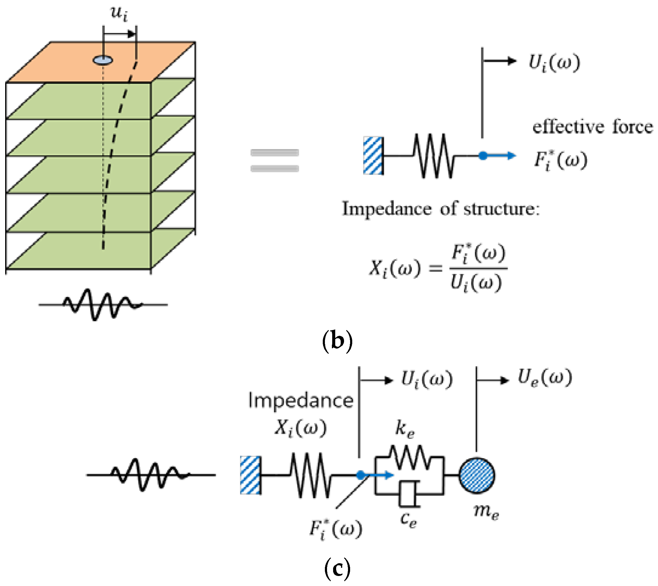
The equation of motion for the structure without equipment, as shown in Figure 2c, can be expressed as Equation (7), which is transformed into Equation (8) in the frequency domain and simplified as Equation (9).

$$\left[\begin{array}{cc}{\mathit{m}}_{\mathit{s}\mathit{s}}& 0\\ \mathbf{0}& m_{ii}\end{array}\right]\left\{\begin{array}{c}{\ddot{\mathit{u}}}_{\mathit{s}}^{*}\\ {\ddot{u}}_i^{*}\end{array}\right\}+\left[\begin{array}{cc}{\mathit{c}}_{\mathit{s}\mathit{s}}& -{\mathit{c}}_{\mathit{s}\mathit{i}}\\ -{\mathit{c}}_{\mathit{i}\mathit{s}}& c_{ii}\end{array}\right]\left\{\begin{array}{c}{\dot{\mathit{u}}}_{\mathit{s}}^{*}\\ {\dot{u}}_i^{*}\end{array}\right\}+\left[\begin{array}{cc}{\mathit{k}}_{\mathit{s}\mathit{s}}& -{\mathit{k}}_{\mathit{s}\mathit{i}}\\ -{\mathit{k}}_{\mathit{i}\mathit{s}}& k_{ii}\end{array}\right]\left\{\begin{array}{c}{\mathit{u}}_{\mathit{s}}^{*}\\ u_i^{*}\end{array}\right\}=-\left\{\begin{array}{c}{\mathit{m}}_{\mathit{s}}{\mathit{l}}_{\mathit{s}}\\ m_{ii}\end{array}\right\}{\ddot{u}}_g$$

(7)

$$\underset{\mathit{I}\mathit{m}\mathit{p}\mathit{e}\mathit{d}\mathit{a}\mathit{n}\mathit{c}\mathit{e}}{\underbrace{\left(\left[\begin{array}{cc}{\mathit{k}}_{\mathit{s}\mathit{s}}& -{\mathit{k}}_{\mathit{s}\mathit{i}}\\ -{\mathit{k}}_{\mathit{i}\mathit{s}}& k_{ii}\end{array}\right]-{\mathit{\omega }}^2\left[\begin{array}{cc}{\mathit{m}}_{\mathit{s}\mathit{s}}& \mathbf{0}\\ {\mathbf{0}}^T& m_{ii}\end{array}\right]+j\omega \left[\begin{array}{cc}{\mathit{c}}_{\mathit{s}\mathit{s}}& -{\mathit{c}}_{\mathit{s}\mathit{i}}\\ -{\mathit{c}}_{\mathit{i}\mathit{s}}& c_{ii}\end{array}\right]\right)}}\left\{\begin{array}{c}{\mathit{U}}_{\mathit{s}}^{*}\\ U_i^{*}\end{array}\right\}=-\left\{\begin{array}{c}{\mathit{m}}_{\mathit{s}}{\mathit{l}}_{\mathit{s}}\\ m_{ii}\end{array}\right\}{\ddot{U}}_g$$

(8)

$$\left(\left[\begin{array}{cc}{\mathit{K}}_{\mathit{s}\mathit{s}}& {\mathit{K}}_{\mathit{s}\mathit{i}}\\ {\mathit{K}}_{\mathit{i}\mathit{s}}& K_{ii}\end{array}\right]\right)\left\{\begin{array}{c}{\mathit{U}}_{\mathit{s}}^{*}\\ U_i^{*}\end{array}\right\}=-\left\{\begin{array}{c}{\mathit{m}}_{\mathit{s}}{\mathit{l}}_{\mathit{s}}\\ m_{ii}\end{array}\right\}{\ddot{U}}_g$$

(9)

where ${\mathit{u}}_{\mathit{s}}^{*}$ is the displacement vector of the structure and $u_i^{*}$ is the displacement at the node to which the equipment is connected. By subtracting Equation (8) from Equation (6), the relation between the equipment–structure interaction force and the corresponding displacement change at the equipment–structure interface is derived as Equation (14) as follows:

$$\left(\left[\begin{array}{cc}{\mathit{K}}_{\mathit{s}\mathit{s}}& {\mathit{K}}_{\mathit{s}\mathit{i}}\\ {\mathit{K}}_{\mathit{i}\mathit{s}}& K_{ii}\end{array}\right]\right)\left\{\begin{array}{c}{\mathit{U}}_{\mathit{s}}-{\mathit{U}}_{\mathit{s}}^{*}\\ U_i-U_i^{*}\end{array}\right\}=\left\{\begin{array}{c}\mathbf{0}\\ F_i\end{array}\right\}$$

(10)

$${\mathit{K}}_{\mathit{s}\mathit{s}}\left({\mathit{U}}_{\mathit{s}}-{\mathit{U}}_{\mathit{s}}^{*}\right)+{\mathit{K}}_{\mathit{s}\mathit{i}}\left(U_i-U_i^{*}\right)=\mathbf{0}$$

(11)

$${\mathit{K}}_{\mathit{i}\mathit{s}}\left({\mathit{U}}_{\mathit{s}}-{\mathit{U}}_{\mathit{s}}^{*}\right)+K_{ii}\left(U_i-U_i^{*}\right)=F_i$$

(12)

$$\left({\mathit{U}}_{\mathit{s}}-{\mathit{U}}_{\mathit{s}}^{*}\right)=-{\mathit{K}}_{\mathit{s}\mathit{s}}^{-1}{\mathit{K}}_{\mathit{s}\mathit{i}}\left(U_i-U_i^{*}\right)$$

(13)

$$X_i\left(U_i-U_i^{*}\right)=F_i$$

(14)

where $X_i$ is the impedance function of the structure expressed as

$$X_i={\mathit{K}}_{\mathit{i}\mathit{i}}-{\mathit{K}}_{\mathit{i}\mathit{s}}{\mathit{K}}_{\mathit{s}\mathit{s}}^{-1}{\mathit{K}}_{\mathit{s}\mathit{i}}$$

(15)

Equation (4), the equation of motion considering the equipment–structure interaction, can be rewritten as Equation (16) by substituting $F_i$ with Equation (14). Equation (16) can be rewritten as a two-DOF equation of motion in the frequency domain, as shown in Equation (17), and the corresponding solution can be obtained as Equation (18).

$$\left[\begin{array}{cc}{K}_{ii}& K_{ie}\\ K_{ei}& K_{ee}\end{array}\right]\left\{\begin{array}{c}{U}_i\\ U_e\end{array}\right\}=-\left\{\begin{array}{c}{F}_i\\ m_e{\ddot{U}}_g\end{array}\right\}=-\left\{\begin{array}{c}{X}_i\left(U_i-U_i^{*}\right)\\ m_e{\ddot{U}}_g\end{array}\right\}$$

(16)

$$\left[\begin{array}{cc}{X}_i+K_{ii}& K_{ie}\\ K_{ei}& K_{ee}\end{array}\right]\left\{\begin{array}{c}{U}_i\\ U_e\end{array}\right\}=\left\{\begin{array}{c}{F}_i^{*}\\ -m_e{\ddot{U}}_g\end{array}\right\}$$

(17)

$$\left\{\begin{array}{c}{U}_i\\ U_e\end{array}\right\}={\left[\begin{array}{cc}{X}_i+K_{ii}& K_{ie}\\ K_{ei}& K_{ee}\end{array}\right]}^{-1}\left\{\begin{array}{c}{F}_i^{*}\\ -m_e{\ddot{U}}_g\end{array}\right\}$$

(18)

where

$$F_i^{*}=X_i{U}_i^{*}$$

(19)

is the effective force that can reproduce the structural response at the interface only caused by the ground motion. The displacements of the structure at the interface and the equipment, $U_i$ and $U_e$, can be calculated using Equation (18), and the relative and absolute accelerations of the equipment can be calculated as follows:

$${\ddot{U}}_e=-{\omega }^2{U}_e$$

(20)

$${\ddot{U}}_{e,total}={\ddot{U}}_e+{\ddot{U}}_g$$

(21)

Equation (17) represents the condition in which the effective force $F_i^{*}$ acts on the two-DOF system illustrated in Figure 2b, where the main structure is replaced by the impedance represented by Equation (15). The impedance $X_i$ and displacement $U_i^{*}$ used to compute $F_i^{*}$ are not dependent on the characteristics of the equipment, as those variables are determined from the equation of motion for the structure itself and its response. Therefore, repeated analyses of the two-DOF system shown in Figure 2b, changing the stiffness of the equipment, allows for the efficient calculation of ISRS considering the equipment–structure interaction effect without repeated analysis of the MDOF coupled model with full DOFs.

3. Structural Modeling

In this study, the ISRS was computed for the auxiliary buildings of the APR 1400 nuclear power plant. An FE model was prepared for the auxiliary building using the commercial software ANSYS, as shown in Figure 3. Both walls and slabs were modeled using a shell element, SHELL1811 of which each node has six DOFs [25]. Basically, a four-node shell element. Mesh was generated automatically using the quadrilateral dominant method so that four-node elements were used mostly and triangular shell elements were included partially [26]. The average mesh size was 3 m, which was determined based on the FE model described in the design report of APR 1400 NPP [27]. The model used in this study comprised 23,569 elements and 1,166,116 DOFs. A fixed boundary condition was applied to constrain the six DOFs of all nodes at the ground level.

3.1. Material Properties

The median compressive strength of concrete was determined in accordance with TR 3002012994, a seismic fragility evaluation guideline [28]. For this purpose, the minimum compressive strength of 91-day concrete given in the APR 1400 design document [27] was converted to the minimum compressive strength of 28-day concrete using the compressive strength curve with respect to time [29]. The median 28-day compressive strength was then calculated by multiplying by 1.25, considering the uncertainty in the cylinder test data [28]. Additionally, the aging factors presented in NEI 07–13 [30] were applied according to the wall and slab thickness so that two different elastic moduli were applied to the auxiliary building model.

$$f_{{cm}_{aging}}^{\prime }=1.2f_{{cm}_{28}}^{\prime } \left(\mathrm{MPa}\right) \mathrm{for} \mathrm{thickness}<0.91 \mathrm{m}$$

(22)

$$f_{{cm}_{aging}}^{\prime }=1.4f_{{cm}_{28}}^{\prime } \left(\mathrm{MPa}\right) \mathrm{for} \mathrm{thickness}>0.91 \mathrm{m}$$

(23)

where $f_{{cm}_{28}}^{\prime }$ and $f_{{cm}_{aging}}^{\prime }$ denote the median 28-day compressive strength and the median compressive strength with the aging effect, respectively. The elastic modulus was calculated using Equation (24), in accordance with ACI 318-08 [31]. The median compressive strength with the aging effect was applied to this equation. The material properties of the cracked and uncracked concrete are summarized in

Table 1. Material properties of concrete.

Property		Thickness < 0.91 m	Thickness > 0.91 m
$f_{cm}^{\prime }{}_{28}$ (MPa)		39.2
$f_{{cm}_{aging}}^{\prime }$ (MPa)		47.04	54.88
$E_C$ (MPa)		32462	35063
Poisson’s ratio		0.17	0.17
Shear modulus (MPa)	Uncracked	13872	14984
	Cracked	6936	7492
Damping ratio (%)	Uncracked	4%	4%
	Cracked	7%	7%

.

$$E_C=4733\sqrt{f_{{cm}_{aging}}^{\prime }} \left(\mathrm{MPa}\right)$$

(24)

3.2. Stiffness & Damping

The stiffness and damping of the reinforced concrete members were determined in accordance with ASCE/SEI 4–16, considering the response level of the overall structure [5]. In ASCE/SEI 4–16, response level 1 does not cause significant cracks, whereas response level 2 causes severe cracks in reinforced concrete structures. Therefore, cracking was evaluated through response spectrum analysis of the uncracked model for an input earthquake.

The cracking strengths for the shear and bending of the walls and slabs were determined in accordance with ACI 349-13 [32]. The cracking strengths for the shear deformation of reinforced concrete shear walls with a height/length ratio of 1.5 or less and 2.0 or higher were assumed to be $0.25\sqrt{f_{{cm}_{28}}^{\prime }}$ and $0.167\sqrt{f_{{cm}_{28}}^{\prime }}$, respectively. The cracking strength was linearly interpolated using the height/length ratio between the two values. Cracking caused by the bending of reinforced concrete walls, floors, or columns was assumed to occur when the flexural tensile stress exceeded $0.623\sqrt{f_{{cm}_{28}}^{\prime }}$.

Table 2. Cracking strength of concrete (MPa).

Shear			Flexure
Aspect ratio	Wall	Slab	Wall and Slab
h/l $\le$ 1.5	1.565	1.043	3.897
h/l $\ge$ 2.0	1.043

summarizes the cracking strengths of the structural members used in this study.

The shear and bending stresses of a slab on the fourth floor and an outer wall in the H2 direction are shown in Figure 4, where the green and red colors represent regions with stress higher than the cracking strength and correspond to cracked concrete, whereas the blue color represents uncracked regions. Most parts of the slab and wall did not experience flexural cracking but exhibited shear cracks, excluding the upper part of the wall. To simplify the numerical model of the auxiliary building, it was assumed that cracking owing to shear deformation occurred in the overall structure. Accordingly, only the shear modulus of the concrete material was reduced by 50%, and 7% of the critical damping corresponding to response level 2 of ASCE/SEI 4–16 was applied to the entire structure.

4. Ground Motion

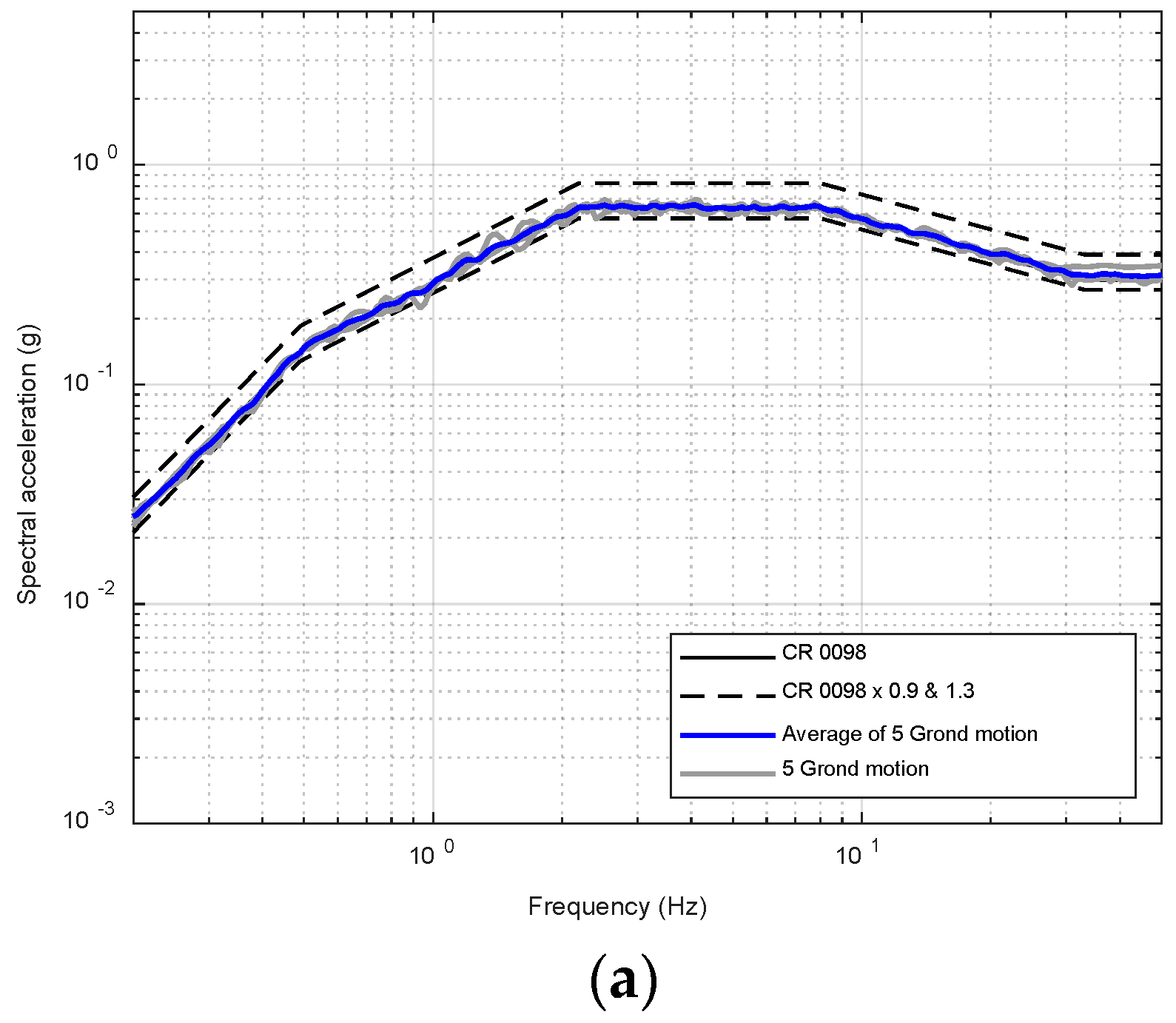
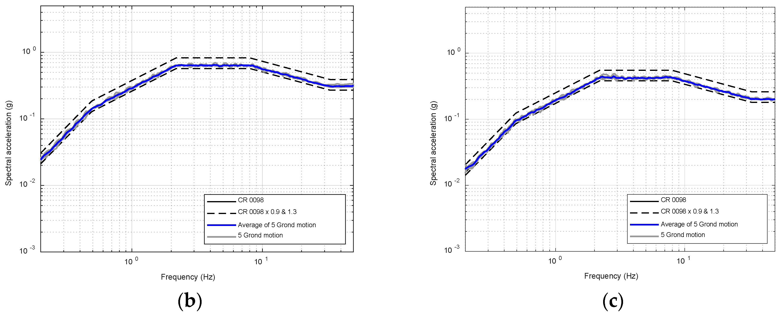
The seismic input to the auxiliary building structure was developed through a site response analysis to consider the site amplification effects. The median response spectrum shape for the 5% damping ratio defined in NUREG/CR-0098 (Newmark and Hall 1978) was adopted as the target response spectrum of bedrock motions [33]. The response spectrum was anchored to a maximum ground acceleration of 0.3 g. The site condition was assumed to be rock, defined by V/A = 36 in·s/g and AD/V² = 6.0, where A is the peak ground acceleration, V is the peak ground velocity, and D is the peak ground displacement D. The target response spectrum of the bedrock is plotted in Figure 5.

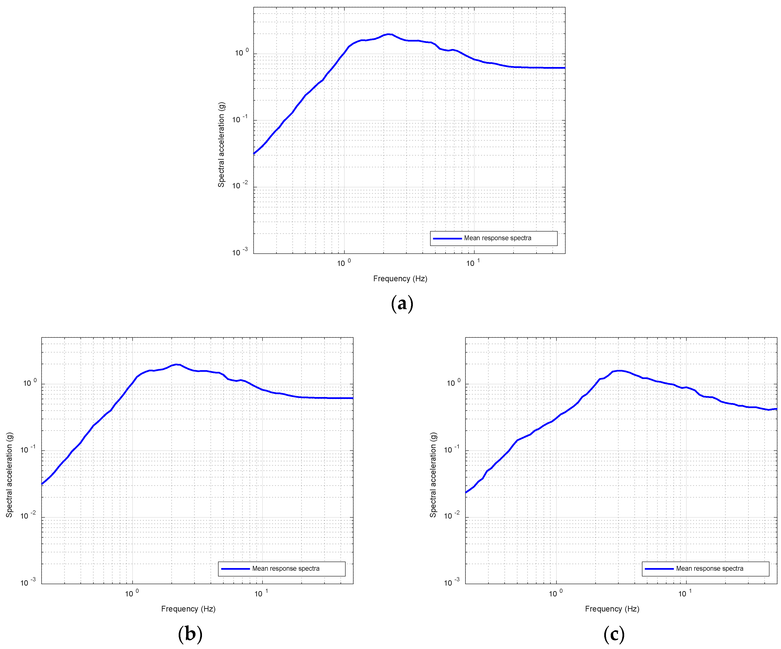
Spectral matching of the recorded ground motions was performed on the target response spectrum. Seed ground motions were selected from a total of 89 sets available from the list of ground motions that are appropriate for matching a rock site with the characteristics of the central and eastern United States (CEUS) presented in NUREG/CR-6728. The selected ground motion sets were matched to the target spectrum, and the five sets with the least change in the waveform were selected. See Jeon et al. (2022) for the detailed selection process [34]. The selected ground motions are listed in

Table 3. Ground motion records.

No	Earthquake Name	Year	Magnitude	Rjb [km]	Vs30 [m/s]
1	Southern Calif	1952	6.00	73.35	493.5
2	Victoria Mexico	1980	6.33	13.8	471.53
3	Northridge-01	1994	6.69	4.92	2016.13
4	Kocaeli Turkey	1999	7.51	31.74	347.62
5	Duzce Turkey	1999	7.14	12.02	293.57

. The mean response spectrum of the five matched ground motions in each direction so that it is between the upper and lower bound defined by 1.3 and 0.9 times the target response spectrum, respectively, as shown in Figure 5 [35].

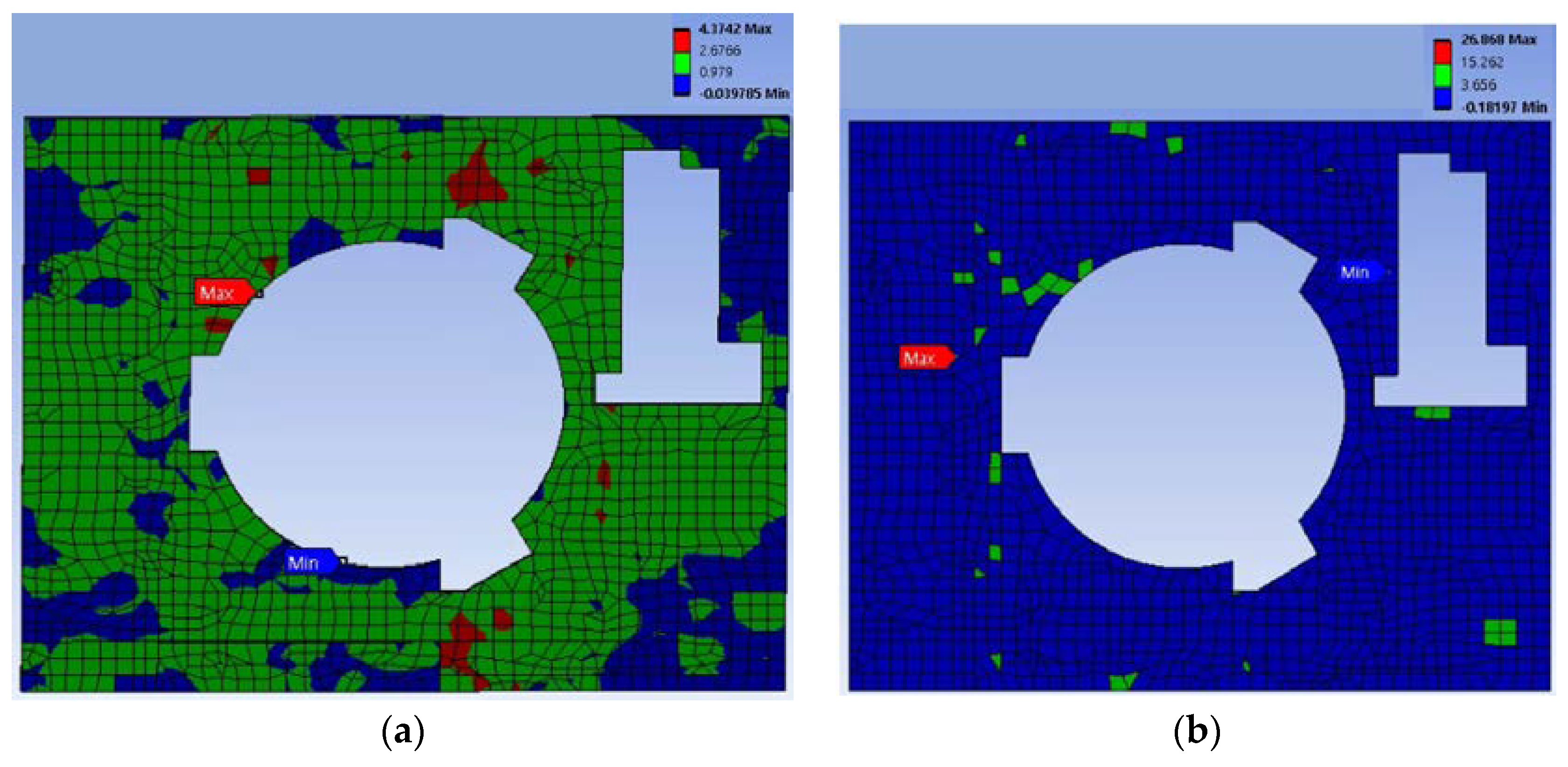
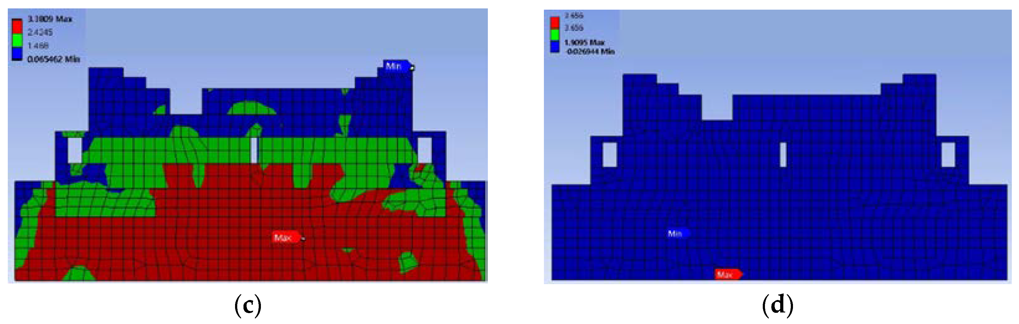
Site response analysis was performed for the shear wave velocity profile S1, one of several profiles applied to the design of the auxiliary building of the APR 1400 nuclear power plant. The free-field surface ground motions from the site response analysis were used as seismic inputs to the base of the structure to calculate the ISRS at a number of locations. In addition, the average response spectrum at the ground surface, as shown in Figure 6, was applied to the crack evaluation analysis described above.

5. In-Structure Response Spectra

5.1. Dynamic Analysis

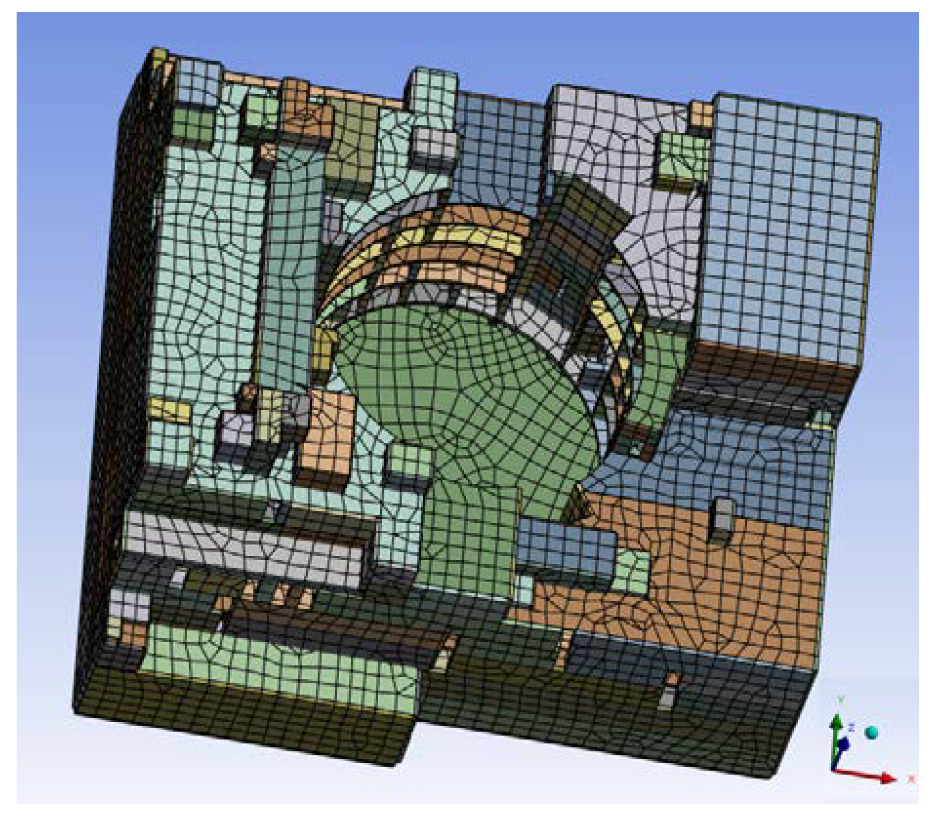
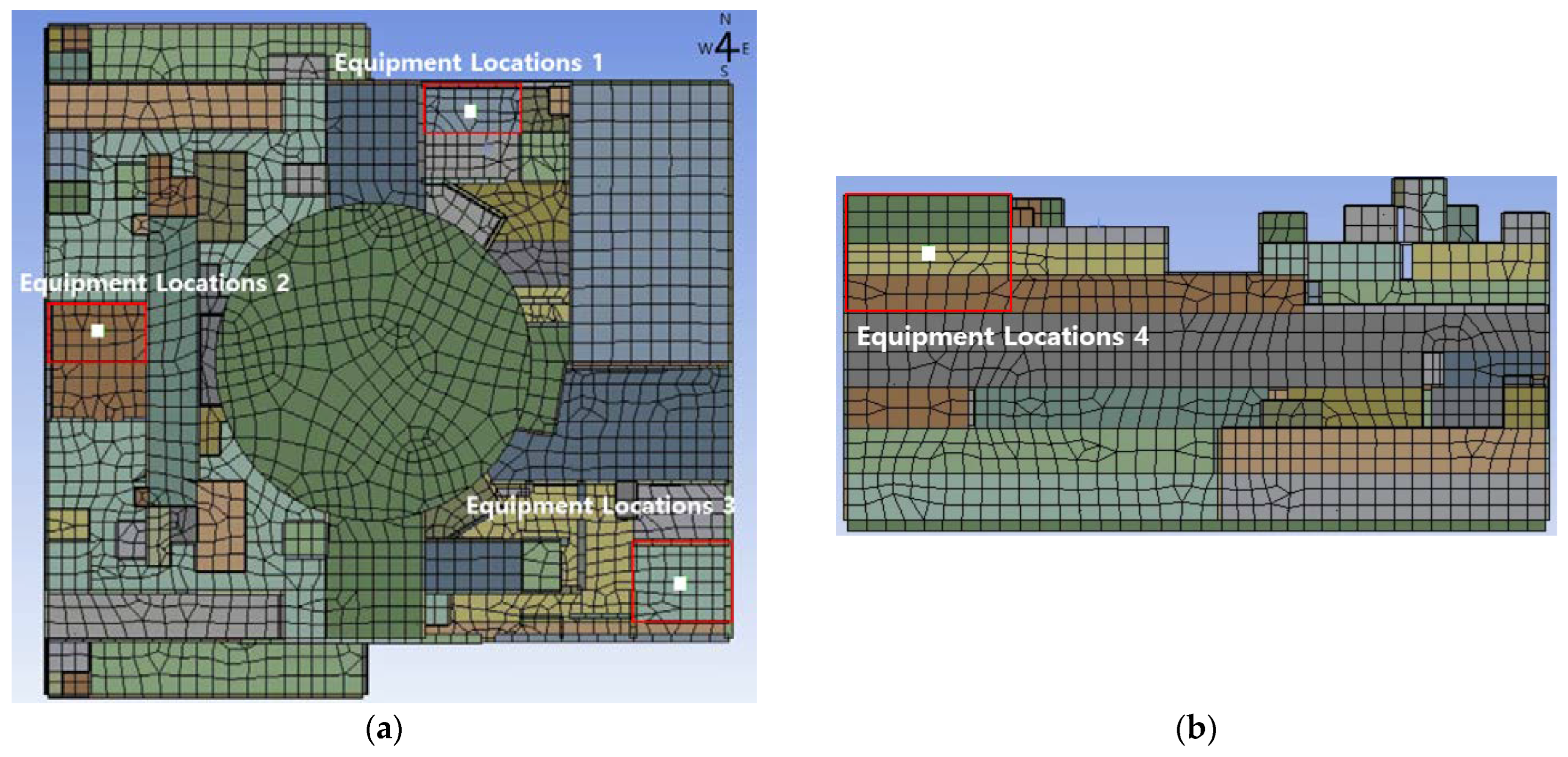
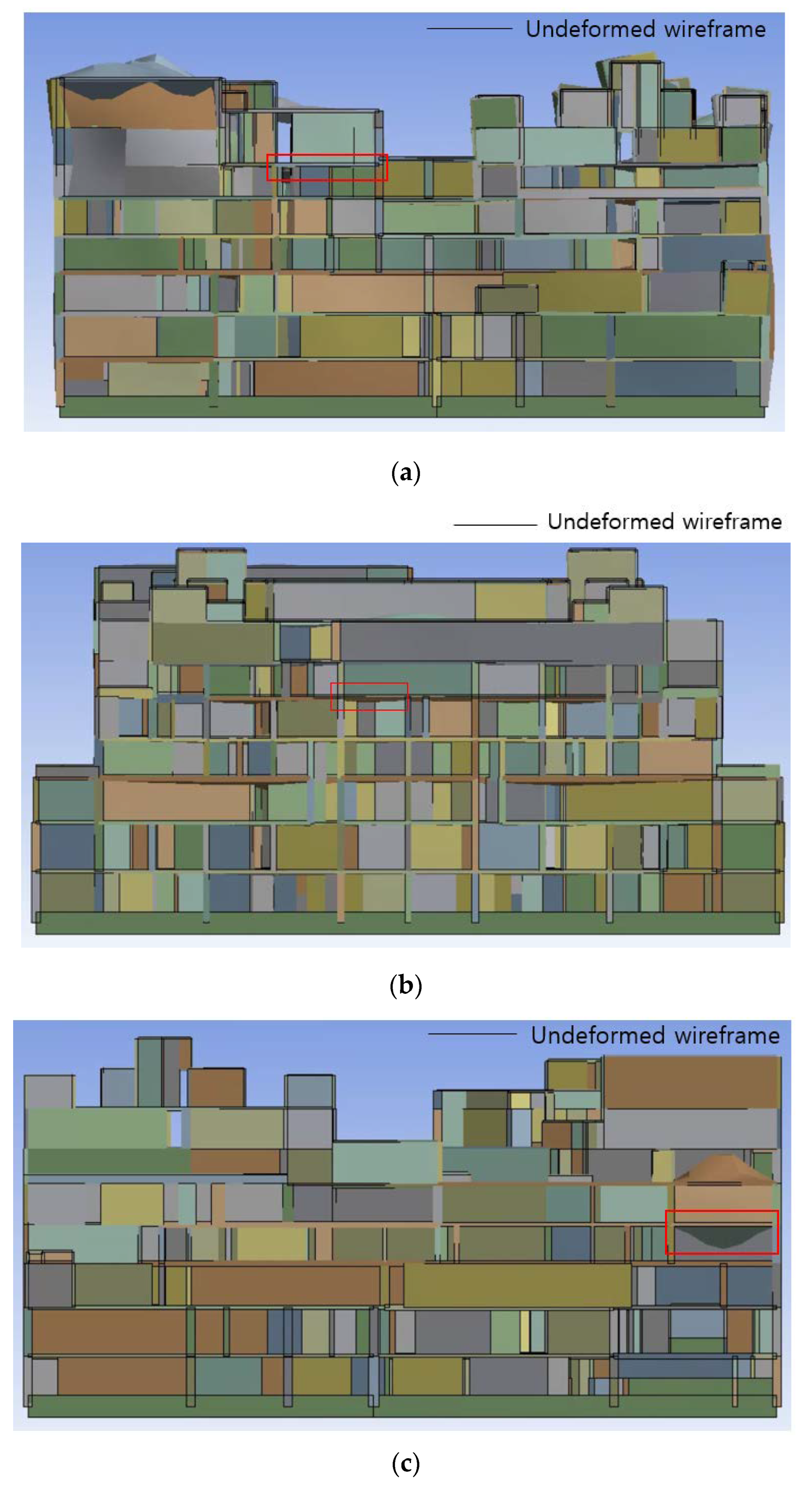
Three slabs and a wall were selected for the location of the equipment where the ISRS was computed, as marked with red boxes in Figure 7. Considering that it is reported that the out-of-plane local vibration has a remarkable equipment–structure interaction effect, a slab with a larger span and a wall with a taller clear height were selected. The ISRS was calculated for two horizontal directions and one vertical direction at the center of each selected slab or wall. The three components of the ground motion were assumed to act simultaneously. Modal time-history analysis was performed using the Newmark method with an assumption of constant acceleration, and a total of 1783 vibration modes were included. The block Lanczos eigenvalue extraction method was adopted for large symmetric eigenvalue problems [36]. The time increment was set as 0.005 s. The mass of the equipment was assumed as 1%, 0.1%, and 0.01% of the entire building mass.

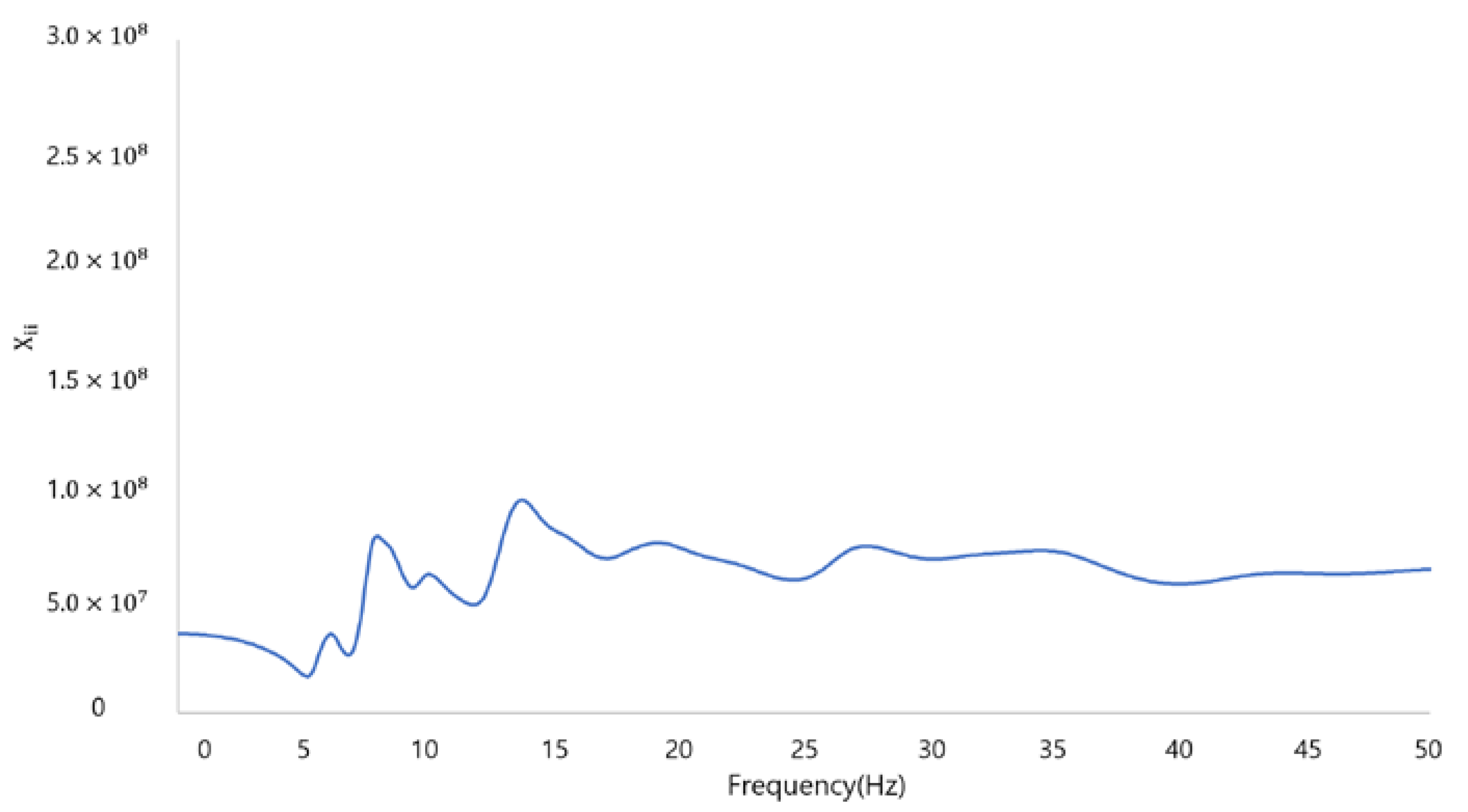
Both decoupled ISRS that does not consider the equipment–structure interaction and coupled ISRS that considers the equipment–structure interaction were calculated and compared at the selected equipment locations. The decoupled ISRS was calculated based on the response acceleration at each equipment location, which was obtained from the response analysis of the auxiliary building decoupled from the equipment represented by Equation (7) using ANSYS. The coupled ISRS was calculated directly as the acceleration response of the coupled two-DOF model represented by Equation (18) using the MATLAB code. For this procedure, the mechanical impedance expressed by Equation (15) was calculated as the inverse of the complex displacement response at the equipment location to the complex harmonic force with unit amplitude at the same node using ANSYS. The mechanical impedance at equipment location 1 in the H1 direction is plotted in Figure 8. It is noted that all ISRS in this study were calculated at frequencies from 0 to 20 Hz with an increment of 0.01 Hz. The equipment frequency was varied by changing the equipment stiffness keeping the equipment mass constant. The mechanical impedance of the primary structure was calculated up to 50 Hz, which is higher than the Nyquist frequency of the 20 Hz oscillator, with an increment of 0.1 Hz.

5.2. Procedure to Calculate ISRS

The overall procedure to calculate ISRS through coupled analysis using a two-DOF system in the frequency domain proposed in this study can be summarized as follows.

Step (1) Uncoupled response analysis of primary structure: Time history analysis of the primary structure is performed for a given ground motion set comprised of two horizontal and one vertical accelerogram and the relative displacement and absolute acceleration responses at the equipment location and in the direction of interest are calculated.

Step (2) Calculation of mechanical impedance: Harmonic analysis of the primary structure is performed for a unit harmonic force acting at the equipment location and in the direction for which the ISRS is calculated. The displacement response is calculated for the same DOF as the input force. The mechanical impedance of the primary structure is calculated as the ratio of the input force to the output displacement at each frequency.

Step (3) Calculation of input to coupled analysis: Fourier transformation of the relative displacement response at the equipment location obtained in Step 1 and the ground acceleration in the direction of interest is performed. Then, the input force to the two-DOF model, $F_i^{*}$, is calculated using Equation (19) in the frequency domain.

Step (4) Coupled analysis using the two-DOF model: Coupled analysis of the two-DOF system is performed using Equation (18) in the frequency domain. The absolute acceleration of the equipment is calculated using Equation (20). Then, the absolute acceleration of the equipment is transformed into the time domain by inverse Fourier transform and the peak absolute acceleration is determined.

Step (5) Calculation of ISRS: Step 4 is repeated for different equipment frequencies where the ISRS is defined. The calculated peak accelerations are plotted with respect to the equipment frequency.

In addition, the following procedure was used to calculate ISRSs using decoupled analysis for comparison in this study.

Step (A) Decoupled analysis using SDOF system: Time history analysis of an SDOF system representing equipment is conducted in the time domain for the base excitation defined by the absolute acceleration response at the equipment location and in the direction of interest calculated in Step 1 for the coupled analysis procedure.

Step (B) Calculation of ISRS: Step A is repeated for different equipment frequencies where the ISRS is defined. The relationship between the peak acceleration of the equipment and the equipment frequency is plotted.

Using a computer with a 32-core CPU and 128-GB RAM, the two-DOF system analysis in the frequency domain spent 65 sec to compute an ISRS corresponding to 200 natural frequencies for a 36-sec-long ground motion set. However, one execution of the modal time history analysis using the full FE model of the auxiliary building with an SDOF oscillator spent 6060 sec. Moreover, the modal time history analysis shall be repeated for 200 natural frequencies of the equipment, which result in 200 × 6060 sec = 337 h. Therefore, the two-DOF system analysis is much more efficient than the conventional coupled analysis using a full FE model.

5.3. Verification of In-Structure Response Spectra and Primary Structure Response

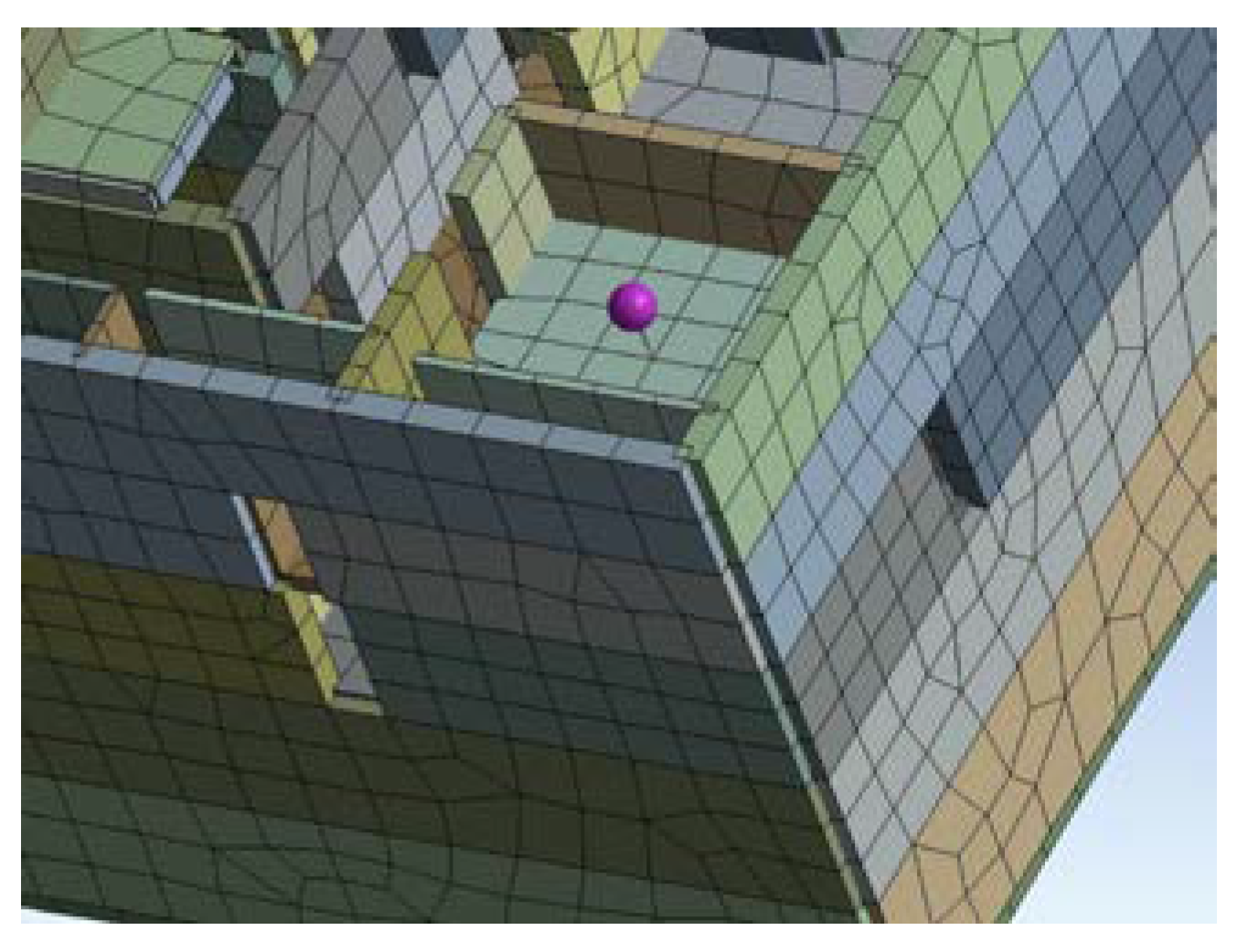
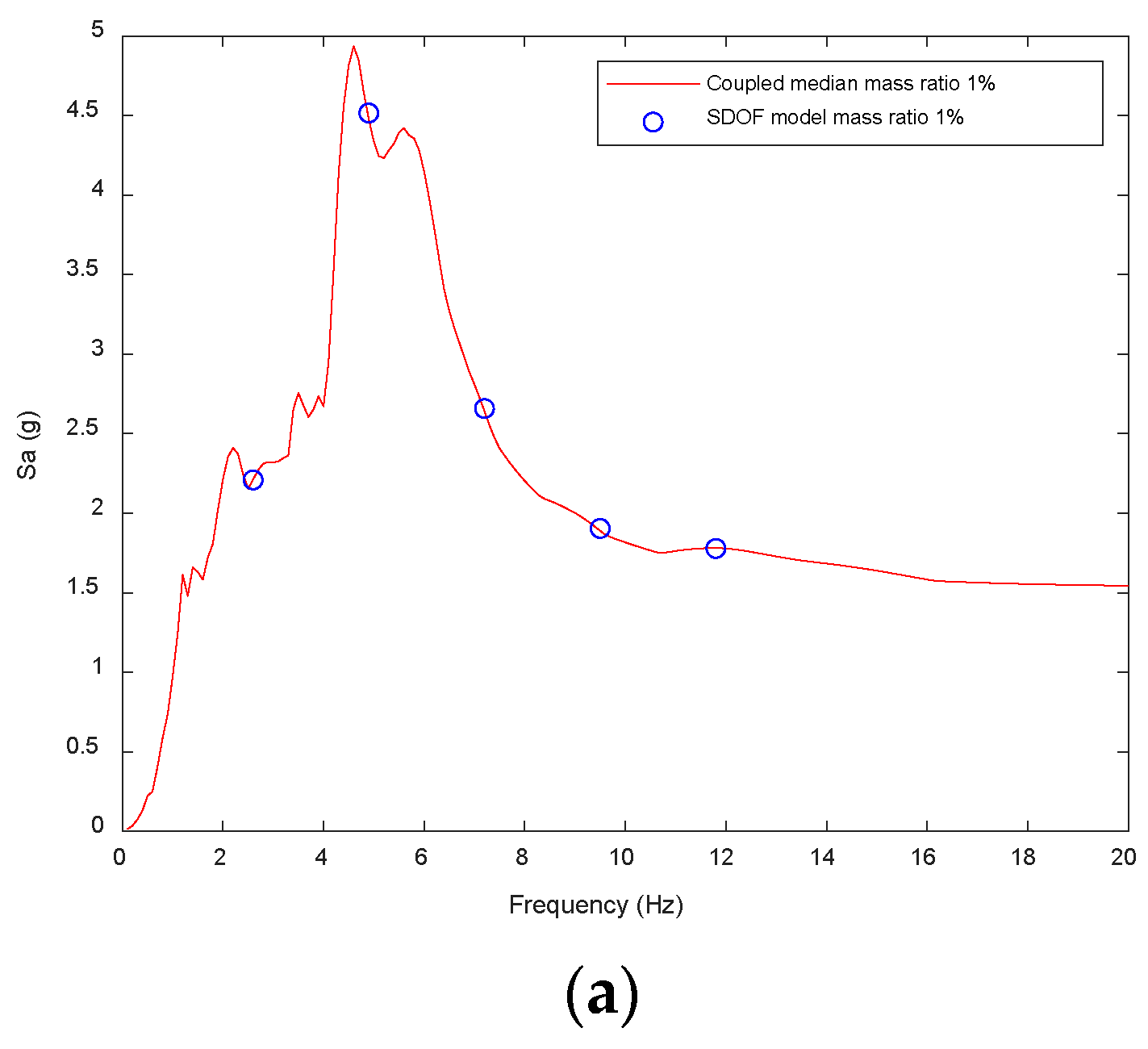
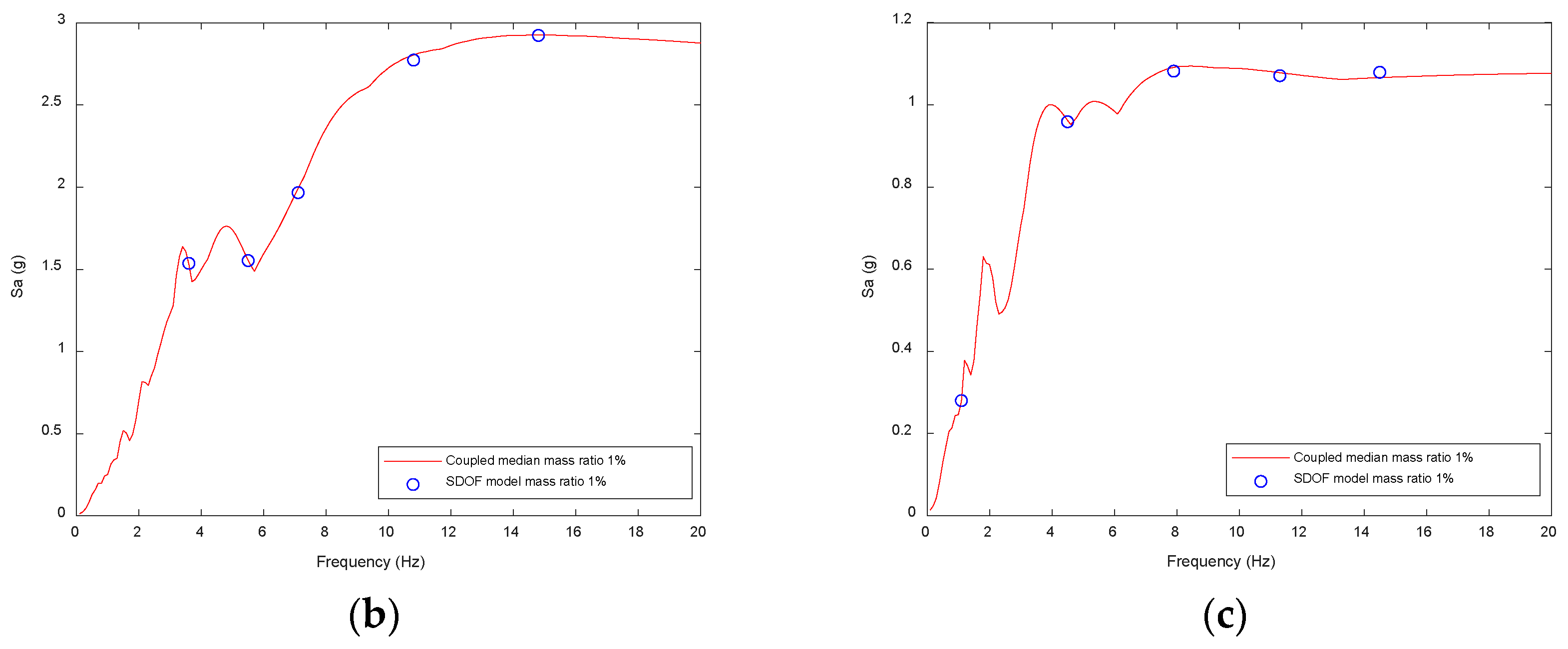
To verify the proposed method for calculating the coupled ISRS, an SDOF oscillator was added to the FE model of the auxiliary building. Using this augmented model, the maximum absolute acceleration response of the added mass in the direction of interest was calculated using time history analysis for the same seismic input. The response of the augmented model was compared with the coupled ISRS obtained by the substructure method for two-DOF analysis in the frequency domain. Verification was performed for the H2- and V-directions at equipment location 2 and the V-direction at equipment location 3. Figure 9 shows the SDOF oscillator located at equipment location 3.

The mass of the SDOF oscillator corresponded to 1% of the entire building mass. Five frequencies were chosen for the frequency of the SDOF oscillator: 2.6, 4.9, 7.2, 9.5 and 11.8 Hz for equipment location 2 in the H2 direction so that the overall tendency of the coupled ISRS, including the frequency at the peak, could be outlined. Different material damping ratios of 7% and 5% were applied to the shell elements of the building and the spring of the oscillator, respectively. The resulting numerical model has the characteristic of non-classical damping; therefore, the time history analysis and harmonic analysis for this verification were performed using the direct integration method. The Newmark method with a constant acceleration assumption was applied as in Section 5.2.

Figure 10 compares the coupled response and ISRS obtained using the substructure technique for different positions and directions. The response acceleration values calculated using the two methods were almost identical at each frequency. Therefore, it can be observed that the two-DOF system analysis using the substructure technique in the frequency domain has sufficient accuracy.

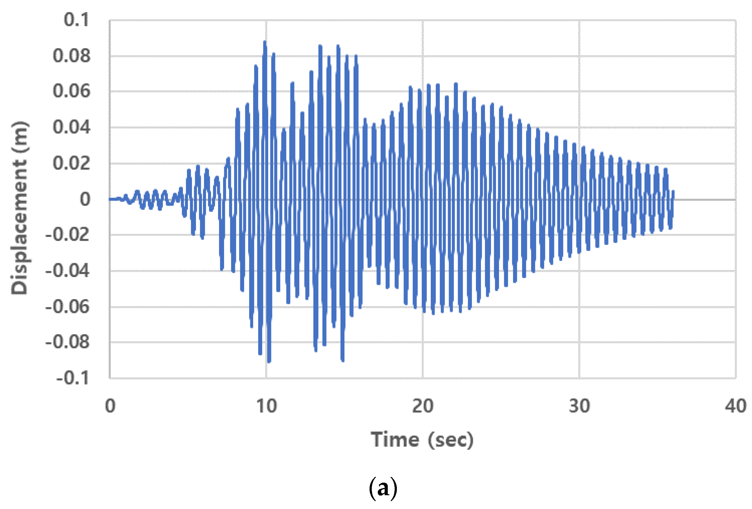
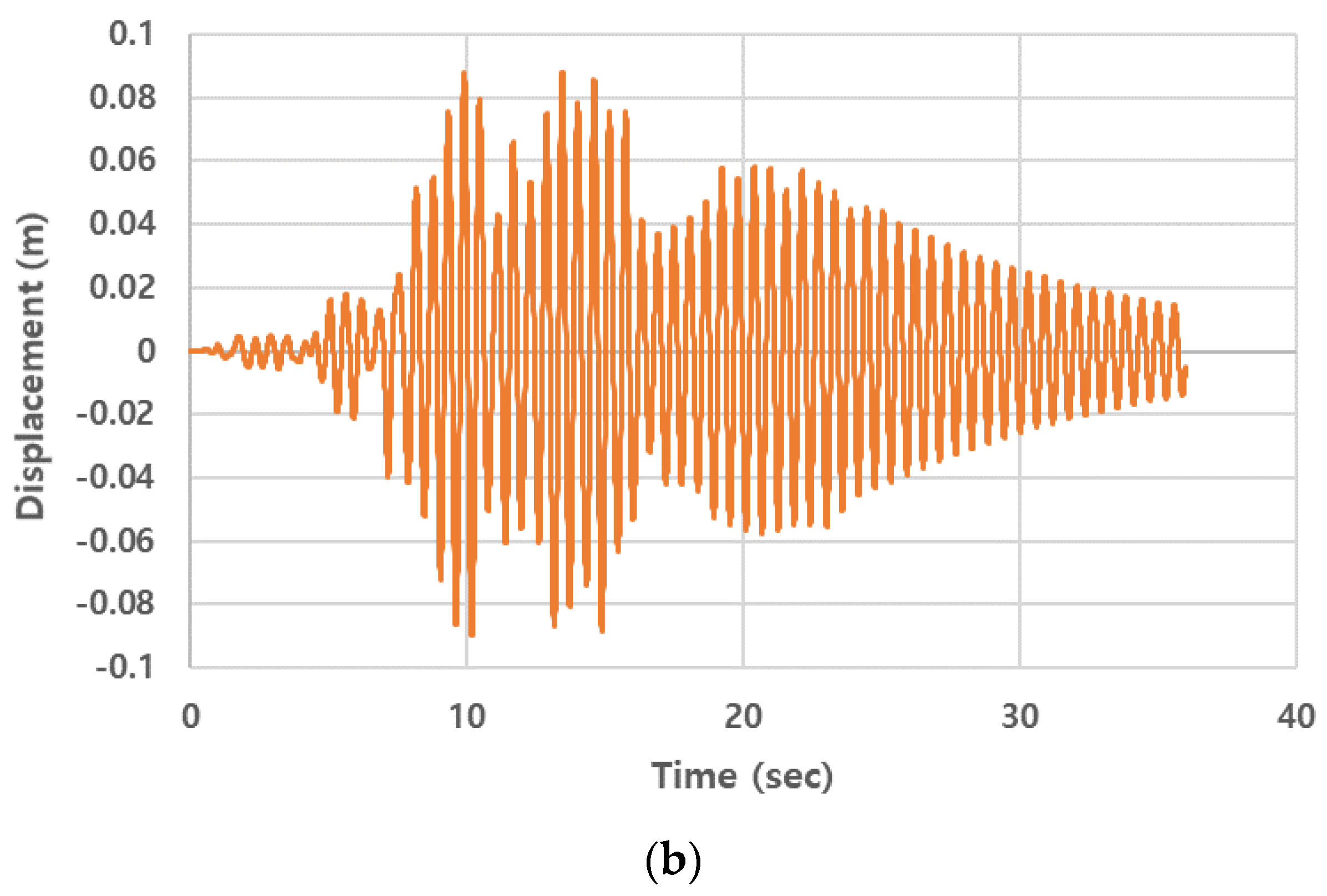
The two-DOF system yields the displacement response of the primary structure in addition to the acceleration response of the secondary system. Among the conditions applied to Figure 10, an oscillator with a 1% mass ratio and 14.5 Hz frequency in the vertical DOF at equipment location 3 was chosen for validation. The displacement of the primary structure at equipment location 3 in the vertical direction was calculated by using the two-DOF system in the frequency domain as well as the full FE model with an SDOF oscillator. The displacement response histories obtained by the two models are almost identical as shown in Figure 11. The peak displacements of the time histories in Figure 11 are 0.08811 m and 0.08815 m, which are almost the same. So, the two-DOF system can yield the primary system response with sufficient accuracy.

5.4. Effect of Equipment Mass

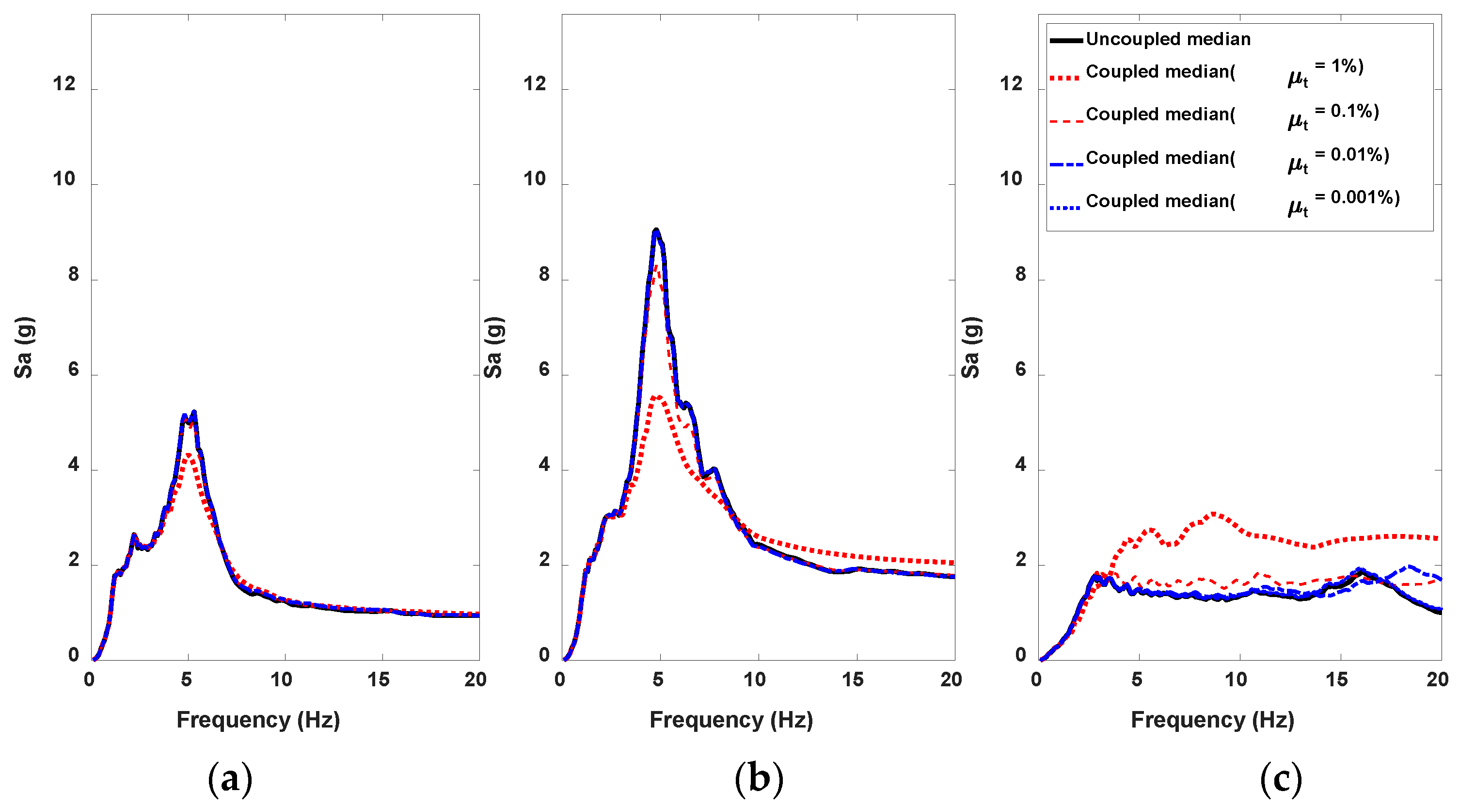
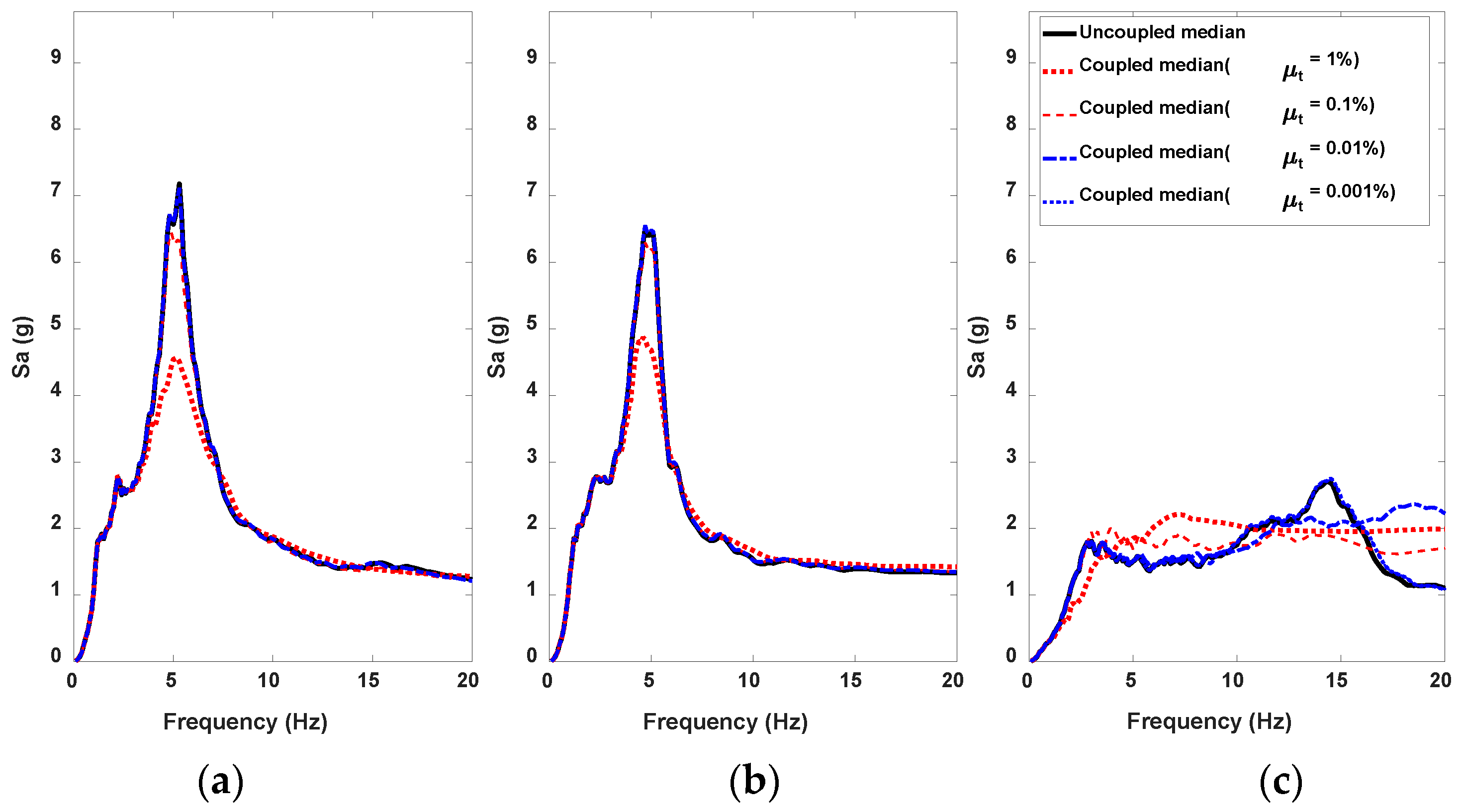
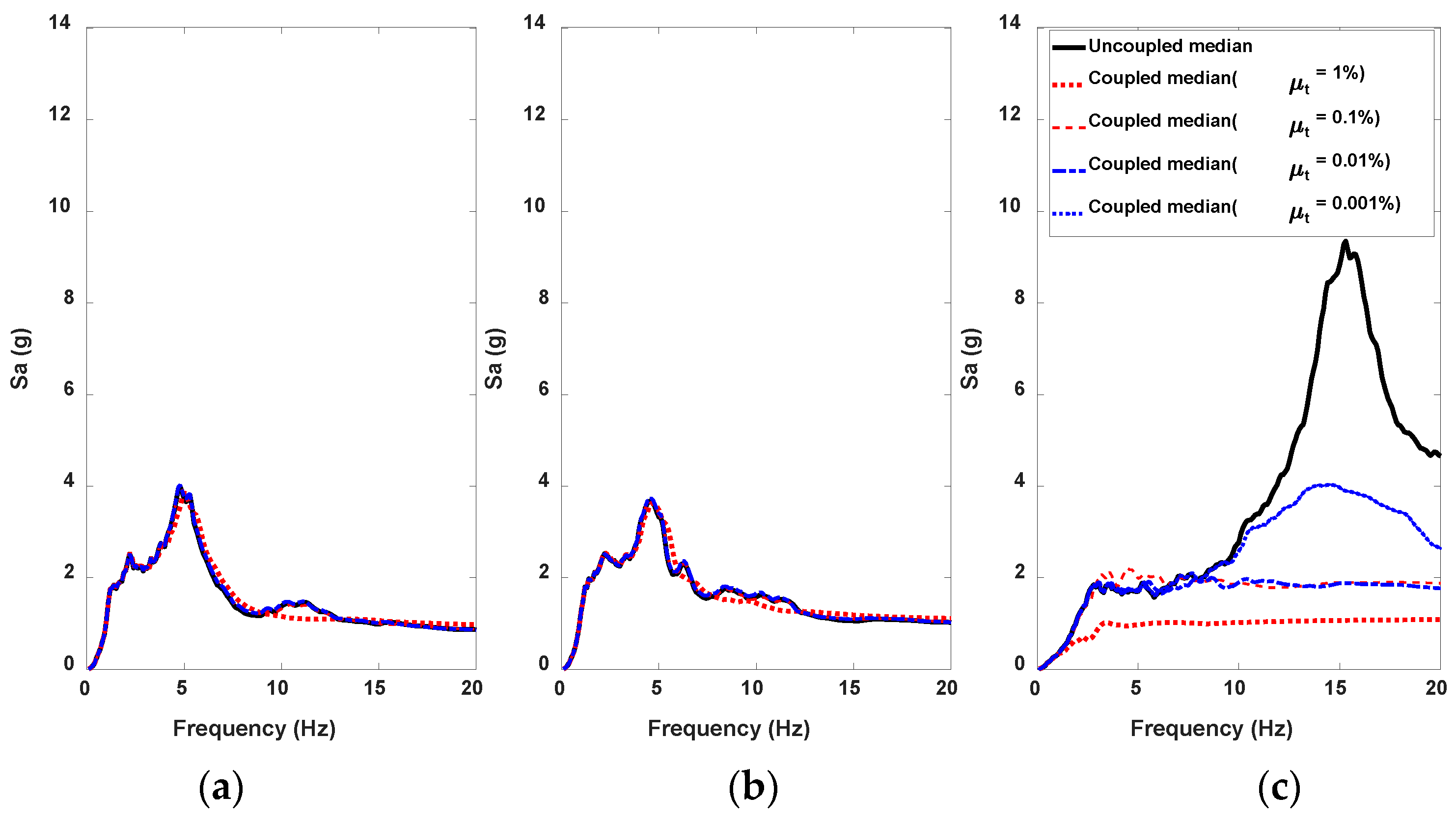
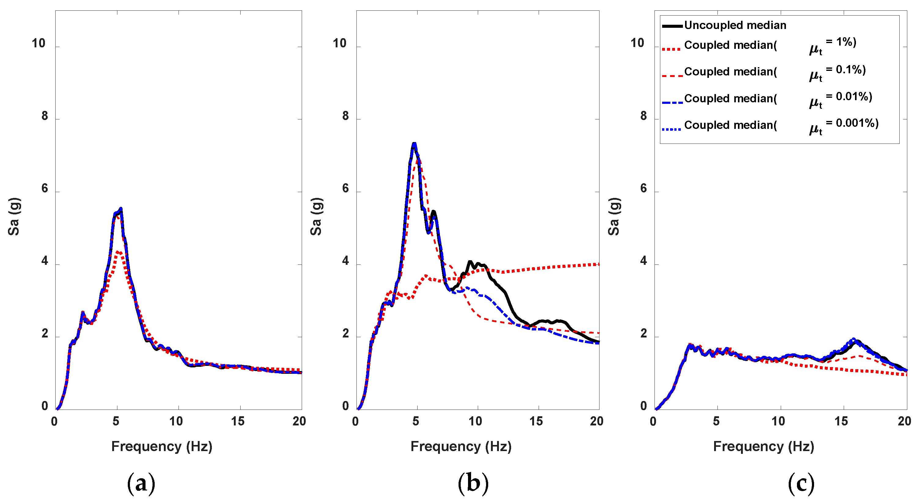
The decoupled and coupled mean ISRS at each of the four equipment locations are compared in Figure 12, Figure 13, Figure 14 and Figure 15, in which the equipment mass is 1%, 0.1%, and 0.01% of the total building mass, and equipment damping is 3%. The ISRS in the H1 and H2 directions at equipment locations 1 and 2 represent in-plane vibration, and as the mass ratio increases, the coupled ISRS decreases below the decoupled ISRS owing to the equipment–structure interaction in the proximity of the dominant frequency. In contrast, the ISRS in the V direction at equipment location 1 represents the out-of-plane vibration, and the acceleration response of the coupled ISRS tends to increase more than that of the decoupled ISRS over frequencies higher than 4 Hz as the mass ratio increases. The V-direction coupled ISRS at equipment location 2, which also represents an out-of-plane vibration, is lower than the decoupled ISRS near the dominant frequency of 15 Hz, but the influence of the mass ratio is unclear. The V-direction coupled ISRS at equipment location 3 showed a significant decrease as the mass ratio increased around the dominant frequency. In the case of the H2-direction coupled ISRS at equipment location 4, representing out-of-plane vibration as well, the equipment–structure interaction effect is noticeable only for 1% mass ratio at a dominant frequency of 5 Hz, while 0.1 and 0.01% mass ratios are more effective at the dominant frequency of 10 Hz. The H1- and V-direction coupled ISRS, representing in-plane vibration, also shows that the equipment–structure interaction becomes more significant as the mass ratio increases.

Figure 16 shows mode shapes corresponding to the dominant frequencies in the V-direction decoupled ISRS for equipment locations 1 to 3. As illustrated in Figure 16a, the dominant mode shape for vertical vibration at equipment location 1 is not as prominent as other parts, and major vertical deformation occurs on the roof and other slabs. In the case of equipment location 2, the local vertical deformation at the location is not prominent compared to other parts too, and the vertical deformation appears to be dispersed in most slabs.

Table 4. Mass ratio of the equipment to the dominant mode for different equipment locations and directions.

Direction	Natural Frequency (Hz)	Equipment Location	Modal Mass (106 kg)	Mass Ratio of the Equipment to the Dominant Mode (%)
				1 (1)	0.1 (1)	0.01 (1)
H1	4.65	3	213,000	994 × 10−6	99.4 × 10−6	9.94 × 10−6
	5.33	1	155	1.37	0.137	0.0137
		2	56.6	3.75	0.375	0.0375
		4	129	1.65	0.165	0.0165
H2	4.65	3	474,000	447 × 10−6	44.7 × 10−6	4.47 × 10−6
	4.97	1	64.0	3.31	0.331	0.0331
		2	124	1.71	0.171	0.0171
		4	129	1.65	0.165	0.0165
V	14.4	2	29.9	7.09	0.709	0.0709
	15.3	3	8.08	26.2	2.62	0.262
	16.1	4	7830	0.0271	0.00271	0.000271
	16.4	1	773	0.274	0.0274	0.00274

⁽¹⁾ Total mass ratio, the equipment mass divided by the total building mass, 212 × 10⁶ kg.

summarizes the modal mass ratio, defined as the ratio of the equipment mass to the modal mass for the dominant frequency in the decoupled ISRS. Three equipment masses corresponding to 1, 0.1, and 0.01% of the total building mass were considered, and these values are denoted by the total mass ratio below: The modal mass ratio of the equipment is expressed by the following equation [5]:

$${\Lambda }_i=M_s/M_{pi}$$

(25)

where

$$M_{pi}={\varphi }_{ci}^{-2}$$

(26)

and $M_s$ is the equipment mass; ${\varphi }_{ci}$ is the value of the i-th mode eigenvector normalized to the mass matrix of the primary structure. It is observed that the modal mass ratio is significantly higher than the total mass ratio for 14.4, and 15.3 Hz, both of which are related to out-of-plane vibration. In the case of vertical vibration, the modal mass of 15.3 Hz vibration mode, of which the deformation is localized to equipment location 3 as shown in Figure 16c, has the smallest value, and the corresponding mass ratio is the highest. On the other hand, the 16.4 Hz mode contains deformations at dispersed locations, as shown in Figure 16a, such that the modal mass is relatively large and the corresponding mass ratios are relatively smaller than those for the 15.3 Hz mode. Overall, it can be noted that the effect of the equipment–structure interaction may be significant for local out-of-plane vibrations.

6. Validation of Decoupling Criteria Considering Mass Ratio and Frequency Ratio of Two-Degree-of-Freedom System

6.1. Decoupling Criteria

In general, coupled analysis considering the equipment–structure interaction causes a difference in the dynamic response of both equipment and structure compared to the decoupled analysis. However, the difference between coupled and decoupled analyses is not always significant enough to warrant the effort and time required for the coupled analysis. ASCE/SEI 4–16 provides decoupling criteria to determine whether the decoupled analysis of a coupled system is acceptable and which model is appropriate among the three types illustrated in Figure 17. Models A and B are models for decoupled analysis, in which the response acceleration of the primary system is used as the input to the secondary system. The only difference between these two models is that in model B, the mass of the secondary system is lumped into the mass of the primary system, as shown in Figure 17b. Model C is a coupled model. The decoupling criteria for selecting an appropriate model are plotted in Figure 18 [5]. Region U allows a decoupled analysis so that all three model types are applicable. In Region C, a coupled analysis should be applied, and only model C is applicable. Region A is an area where the response error of Model A increases, and only Models B and C are applicable. Region B is an area where the response error of Model B increases, with only Models A and C being acceptable.

The solid boundaries between regions U and A and between regions B and C in Figure 18 are expressed by the following equation based on Hadjian and Ellison (1986) [37]:

$$\frac{{\omega }_e}{{\omega }_s}=\left|\sqrt{\frac{a^2-2a}{2a\left(1-{\mu }_A\right)-4}}\right|$$

(27)

where

$$a=\frac{2}{{\left(1-e_A\right)}^2}$$

(28)

and ${\omega }_e$ is the natural frequencies of the equipment; ${\omega }_s$ is the natural frequency of the decoupled structure in Model A; ${\mu }_A$ is the modal mass ratio calculated for the modal mass of Model A; $e_A$ is the acceptable error in the natural frequency predicted by Model A compared to that calculated by the coupled Model C. The dashed boundaries between regions U and B and between regions A and C in Figure 18 are expressed by the following equation [37]:

$$\frac{{\omega }_e}{{\omega }_l}=\left|\sqrt{\frac{{\left(1+{\mu }_B\right)}^{-1}-b}{\left(b-b^2\right)}}\right|$$

(29)

where

$$b={\left(1-e_B\right)}^2$$

(30)

and ${\omega }_l$ is the natural frequency of the structure with lumped equipment mass in Model B; ${\mu }_B$ is the modal mass ratio calculated for the structure with the lumped equipment mass in Model B; $e_B$ is the acceptable error in the natural frequency predicted by Model B compared to that calculated by the coupled model C. Equations (27) and (29) represent the relationship between the frequency ratio and the modal mass ratio for the acceptable error in the prediction of the coupled natural frequency using decoupled Model A and B, respectively. Figure 18 was plotted for $e_A=e_B=0.1$, as adopted in ASCE/SEI 4–16 [4], assuming that the error between the frequency of the coupled model and the frequency predicted by model A or B shall be less than 10%. The structural response error from the modeling technique selected using Figure 18 may be large, but it always yields conservative results according to ASCE/SEI 4–16 and Hadjian and Ellison (1986) [5,37].

Considering the indirect relation between ASCE/SEI 4–16 criteria and actual equipment response, additional decoupling criteria were investigated in this study. US NRC adopted decoupling criteria in NUREG-75/087 (1975) based on Hadjian and Ellison’s criteria with $e_A=e_B=0.05$, which is stricter than ASCE/SEI 4–16 [22]. In addition, US NRC simplified Hadjian and Ellison’s criteria using linear lines as shown in Figure 19 and combined Region A, B and C as a single coupling-required region. As a result, the coupling-required region that begins at the mass ratio 0.01 was extended compared to ASCE/SEI 4–16 criteria. It is noted that US NRC decoupling criteria do not specify a model type between A to C in Figure 19 required for coupled analysis. Fouquiau et al. (2018) proposed new criteria based on a 5% change in the spectral displacement of the primary system between the uncoupled and coupled models, of which both primary and secondary systems are SDOF systems [23]. The decoupling criteria separate the plane of mass ratio and frequency ratio into four regions as shown in Figure 19 like ASCE/SEI 4–16 criteria, but using solid lines. However, region C where explicit coupled modeling is required is extended remarkably compared to ASCE 4–16 criteria.

6.2. Validation of Decoupling Criteria Based on Two-Degree-of-Freedom System

In this section, we examine whether the difference in responses between the coupled and decoupled analyses conforms to the three representative decoupling criteria for determining the necessity of the coupled analysis.

First, the equipment locations and frequencies for applying the decoupling criteria were selected as the frequency at which the response difference between the decoupled and coupled analyses was significant, as shown in Figure 12, Figure 13, Figure 14 and Figure 15. Essentially, the frequency at the peak of the decoupled ISRS was selected for the following conditions: H2-directional ISRS at equipment location 1, V-directional ISRS at equipment location 2, V-directional ISRS at equipment location 3, of which total mass ratio ${\mu }_T$ are 1, 0.1, and 0.001%, respectively. The selected equipment frequencies and corresponding response reduction rates are shown in Figure 20, where $f_{pA}$ and $f_{pB}$ represent the frequency at the peak of ISRS using Models A and B, respectively. In addition, $f_{ucA}$ and $f_{ucB}$ represent the frequency where the coupled ISRS yielded an unconservative response compared to uncoupled ISRS using Models A and B, respectively, and located in a relatively flat part of the ISRS. The peaks of uncoupled ISRS at $f_{pA}$ and $f_{pB}$ decreased by 29.8–65.3% using the coupled analysis. Meanwhile, the spectral accelerations of uncoupled ISRS at $f_{ucA}$ and $f_{ucB}$ increased by 20.2–42.1% using the coupled analysis. In other words, the selected conditions include both conservatism and non-conservatism that can exist in the coupled analysis.

For the selected frequencies in Figure 20, combinations of the frequency ratio and modal mass ratio are plotted with the decoupling criteria expressed by Equations (27) and (29) in Figure 21, where $f_{pA}$, $f_{pB}$, $f_{ucA}$ and $f_{ucB}$ are marked in the corresponding figure in Figure 20. All 1783 vibration modes of the auxiliary building structure with a natural frequency from 3.4 to 75.9 Hz calculated in the eigenvalue analysis were included to plot Figure 20. However, in Figure 21c, the mass ratio was limited to those higher than $1.0\times {10}^{-4}$ to concentrate on major modes with relatively higher mass ratios. Except for equipment frequencies $f_{pA}=f_{pB}$ and $f_{ucA}$ in Figure 21b, all points are located inside the region U, where coupled analysis is not required. However, as shown in Figure 20, the response obtained by the coupled analysis is significantly different from that of the decoupled analysis using Models A or B. In particular, the spectral acceleration at a number of selected equipment frequencies obtained by coupled analysis was 20–42% higher than that obtained by decoupled analysis using Models A or B.

Two additional decoupling criteria by US NRC and Fouquiau et al. were applied to the same combinations of the frequency ratio and modal mass ratio mentioned above and the results are plotted in Figure 22. Most selected equipment frequencies denoted by $f_{pA}, f_{pB}, f_{ucA}$ and $f_{ucB}$ in each figure are related to one or more modes of which frequency ratio and modal mass ratio are located inside regions requiring coupled analysis by both US NRC and Fouquiau et al. criteria. However, for the equipment frequency $f_{pB}$ in Figure 22c, all points are outside the coupling-required region of the US NRC criteria, but two of those points are inside Region C of Fouquiau et al. criteria. Therefore, Fouquiau et al. criteria can distinguish coupling-required equipment conditions the most adequately among the three criteria in comparison. It is notable that US NRC criteria are sufficient to distinguish equipment conditions for which decoupled analysis yields unconservative results such as equipment frequency $f_{ucA}$ and $f_{ucB}$ in Figure 22a–c although the accuracy of the equipment response can be significantly improved by coupled analysis as shown in Figure 20. Finally, in the case of $f_{ucB}$ in Figure 22b, it is observed that only one point is located inside Region C but many points are located inside the coupling-required area of US NRC criteria. Therefore, for robust decision-making, a combination of US NRC and Fouquiau et al. criteria marked with thicker solid lines in Figure 19 is recommended to define a region where explicit coupled analysis is required.

7. Conclusions

This study investigated the applicability of a coupled analysis method based on a substructuring technique to calculate the ISRS for a nuclear power plant structure. The model of the primary structure was condensed into an impedance function and combined with the equipment represented by an SDOF oscillator in the frequency domain. The resulting two-DOF system was used to efficiently calculate the coupled ISRS without repeated analysis of the full model. This coupled analysis method was applied to a finite element model of an auxiliary building in a nuclear power plant to validate both the accuracy and impact on the equipment response. In addition, three representative decoupling criteria to determine the acceptability of the decoupled analysis were applied to the auxiliary building to examine whether they were consistent with the coupled analysis results. The conclusions obtained from this study are summarized as follows:

(1)

The acceleration and displacement response of the coupled model composed of an SDOF oscillator and a full MDOF building model matched the ISRS and primary structure displacement obtained through the two-DOF system, respectively.

(2)

The acceleration response around the dominant peaks in the coupled ISRS tended to decrease as the modal mass ratio between the equipment and structure increased. However, in other frequency regions, a larger mass can increase the acceleration response.

(3)

Even for equipment with the same mass, the response change between the coupled and decoupled analyses varies depending on the installation position and direction of motion. The response reduction was more prominent, as the deformation in the mode shape was locally concentrated within a limited region where the equipment was installed.

(4)

Decoupled analysis may overestimate responses significantly near the peak of ISRS and underestimate responses relatively far from the peak by more than 20% compared to the coupled analysis, although the decoupled analysis is permitted in accordance with the decoupling criteria adopted in ASCE 4–16. Therefore, the decoupling criteria need to consider the response change more directly than the natural-frequency change.

(5)

Decoupling criteria more conservative than ASCE/SEI 4–16 or considering the response change directly, such as US NRC or Foucuiau et al. criteria, are more adequate. In support of this, decoupling criteria defined by combining US NRC and Foucuiau et al. criteria distinguished significant response change by coupled analysis the most comprehensively in the example NPP auxiliary building analysis, and are recommended to be used.

(6)

An attempt to perform coupled analysis is recommended regardless of the decoupling criteria when decoupled analysis yields excessive equipment response owing to resonance with localized vibration modes.

References

1. Chen, Y.; Soong, T.T. Seismic Response of Secondary Systems. Eng. Struct. 1988, 10, 218–228. [Google Scholar] [CrossRef]
2. Perez, Y.M.; Guerra, E.M.; Bazan-Zurita, E. Seismic Response of Equipment Supported on Structure. In Proceedings of the 23rd Conference on Structural Mechanics Reactor Technology (Transaction SMiRT-23), Manchester, UK, 10–14 August 2015. Paper ID 670. [Google Scholar]
3. Gupta, A.; Gupta, A.K. New developments in Coupled Seismic Analysis of Equipment and Piping. In Proceedings of the Transactions of the 13th International Conference on Structural Mechanics in Reactor Technology, SMiRT-13, Porto Alegre, Brazil, 13–18 August 1995. [Google Scholar]
4. Gupta, A. Seismic Response of Secondary Systems. Ph.D. Thesis, North Carolina State University, Raleigh, NC, USA, 1996. [Google Scholar]
5. ASCE Standard 4-16; Seismic Analysis of Safety-Related Nuclear Structures. American Society of Civil: Reston, VA, USA, 2017.
6. Rev. 3. NUREG-0800; Seismic System Analysis Standard Review Plan 3.7.2. U.S. Nuclear Regulatory Commission: Washington, DC, USA, 2007.
7. Liu, Y.; Wang, X.; Wang, X.; Zhang, X.; Gong, W. Floor Response Spectra Analysis of a Nuclear Reactor Considering Uncertainties in Soil Parameter. Structure 2022, 37, 305–317. [Google Scholar] [CrossRef]
8. Merino, R.M.; Perrone, D.; Filiatrault, A. Consistent Floor Response Spectra for Performance-based Seismic Design of Nonstructural Elements. Earthq. Eng. Struct. Dyn. 2020, 49, 261–284. [Google Scholar] [CrossRef]
9. Jiang, W.; Li, B.; Xie, W.C. Generate Floor Response Spectra: Part 1. Direct Spectra-to-Spectra Method. Nucl. Eng. Des. 2015, 2933, 525–546. [Google Scholar] [CrossRef]
10. Li, B.; Jiang, W.; Xie, W.C.; Pandey, M.D. Generate Floor Response Spectra, Part 2: Response Spectra for Equipment-Structure Resonance. Nucl. Eng. Des. 2015, 293, 547–560. [Google Scholar] [CrossRef]
11. Wang, R.; Xie, W.C.; Pandey, M.D. Generation of Floor Response Spectra Structures under Seismic Excitations at Multiple Supports. Nucl. Eng. Des. 2022, 389, 111527. [Google Scholar] [CrossRef]
12. Tseng, W.S. Equipment Response Spectra Including Equipment-Structure Interaction Effects. In Proceedings of the 1989 ASME Pressure Vessels and Piping Conference, Honolulu, HI, USA, 23–27 July 1989; Volume 155, pp. 21–29. [Google Scholar]
13. Choi, D.H.; LEE, S.H. Generation of Floor Response Spectra including Equipment-Structure Interaction in Frequency Domain. J. Eng. Soc. Korea 2005, 9, 13–19. [Google Scholar]
14. Cho, S.G.; Gupta, A. Generation of Floor Response Spectra Considering Coupling Effect of Primary and Secondary System. J. Earthq. Eng. Soc. Korea 2020, 24, 179–187. [Google Scholar] [CrossRef]
15. Kwag, S.Y.; Eem, S.H.; Jung, K.S.; Jung, J.W.; Choi, I.K. A Study on the Effects of Nuclear Power Plant Structure-Component Interaction in Component Seismic Responses. J. Comput. Struct. Eng. Inst. Korea 2022, 35, 83–91. [Google Scholar] [CrossRef]
16. Jayarajan, P. Equipment-Structure Interaction and its Effect on Seismic Demand. IOSR J. Mech. Civ. Eng. IOSR-JMCE 2019, 16, 44–50. [Google Scholar]
17. Dubey, A.R.; Bodda, S.; Gupta, A.; Vasquez, J.; Bhargava, D. Reduction in Seismic Demand by Using Equipment-Structure Interaction. In Proceedings of the 25th International Conference on Structural Mechanics in Reactor Technology, SMiRT-25, Charlotte, NC, USA, 4–9 August 2019. Division V. [Google Scholar]
18. EPRI TR-3002009429; Advanced Nuclear Technology: High-Frequency Seismic Loading Evaluation for Standard Nuclear Power Plants. Electric Power Research Institute: Washington, DC, USA, 2017.
19. Bazan-Zurita, E.; Jarernprasert, S.; Guerra, E.; Rizzo, P.C. Assessment of Resultant Earthquake In-Structure Response Spectra. In Proceedings of the 23rd International Conference on Structural Mechanics in Reactor Technology, SMiRT-23, Manchester, UK, 10–14 August 2015. Division V. [Google Scholar]
20. Jha, S.; Roshan, A.D.; Bishnoi, L.R. Floor Response Spectra for Beyond Design Basis Seismic Demand. Nucl. Eng. Des. 2017, 323, 256–268. [Google Scholar] [CrossRef] [Green Version]
21. Rahman, M.M.; Nahar, T.T.; Kim, D.; Park, W. Location Sensitivity of Non-structural Component for Channel-type Auxiliary Building Considering Primary-secondary Structure Interaction. Int. J. Eng. Trans. A Basics 2022, 35, 1268–1282. [Google Scholar]
22. NUREG-75/087; Standard Review Plan for the Review of Safety Analysis Reports for Nuclear Power Plants. U.S. Nuclear Regulatory Commission: Washington, DC, USA, 1975.
23. Fouquiau, P.V.; Barbier, F.; Chatzigogos, C. New Dynamic Decoupling Criteria for Secondary Systems. In Proceedings of the 16th European Conference on Earthquake Engineering, Thessaloniki, Greece, 18–21 June 2018; pp. 1–10. [Google Scholar]
24. Jung, K.S.; Kwag, S.Y.; Choi, I.K.; Eem, S.H. Analysis of Seismic Response due to Dynamic Coupling Between a Primary Structure and Secondary System. J. Earthq. Eng. Soc. Korea 2020, 24, 87–93. [Google Scholar] [CrossRef]
25. ANSYS, Inc. Element Reference 2021, Release 21.1, Ansys Mechanical; ANSYS, Inc.: Canonsburg, PA, USA, 2021. [Google Scholar]
26. ANSYS, Inc. Meshing Users Guide 2021, Release 21.1, Ansys Mechanical; ANSYS, Inc.: Canonsburg, PA, USA, 2021. [Google Scholar]
27. Rev. 0. APR1400-k-X-FS-14002-NP; APR1400 Design Control Document Tier 2, Chapter 3—Design of Structure, System, Components, and Equipment. Korea Electric Power Corporation and Korea Hydro & Nuclear Power Co., Ltd.: Naju, Korea, 2014.
28. EPRI 3002012994; Seismic Fragility and Seismic Margin Guidance for Seismic Probabilistic Risk Assessments. Electric Power Research Institute (EPRI): Palo Alto, CA, USA, 2018.
29. Troxell, G.E.; Davis, H.E.; Kelly, J.W. Composition and Properties of Concrete, 2nd ed.; McGraw-Hill: New York, NY, USA, 1968. [Google Scholar]
30. NEI 07-13; Methodology for Performing Aircraft Impact Assessments for New Plat Designs. Nuclear Energy Institute: Washington, DC, USA, 2009.
31. ACI 318R-08; ACI Committee 318, Building Code Requirements for Structural Concrete (ACI 318-08) and Commentary. American Concrete Institute: Farmington Hills, MI, USA, 2008.
32. ACI 349-13; ACI Committee 349, Code Requirements for Nuclear Safety-Related Concrete Structures and Commentary. American Concrete Institute: Farmington Hills, MI, USA, 2013.
33. Newmark, N.M.; Hall, W.J. Development of Criteria for Seismic Review of Selected Nuclear Power Plants; U.S. Nuclear Regulatory Commission: North Bethesda, MS, USA, NUREG/ CR-0098, 1978. [Google Scholar]
34. Jeon, S.H.; Shin, D.H.; Park, J.H. Seismic Response of a NPP Containment Building Analyzed Using Ground Motion Records with Different Indices of Wave Characteristic Changes. J. Korea Concr. Inst. 2022, 34, 299–310. [Google Scholar] [CrossRef]
35. NUREG-0800; US Nuclear Regulatory Commission Standard Review Plan 3.7.1. Revision 4. U.S. Nuclear Regulatory Commission: Washington, DC, USA, 2014.
36. ANSYS, Inc. Theory Reference, 2021, Release 21.1, Ansys Mechanical; ANSYS, Inc.: Canonsburg, PA, USA, 2021. [Google Scholar]
37. Hadjian, A.H.; Ellison, B. Decoupling of Secondary Systems for Seismic Analysis. Transactions of the ASME. J. Press. Vessel. Technol. 1986, 108, 78–85. [Google Scholar] [CrossRef]
Figure 1. Procedure of calculating ISRS.
Applsci 13 00247 g001
Figure 2. Coupled model considering equipment–structure interaction: (a) Coupled system with full DOFs; (b) Decoupled system and corresponding mechanical impedance function; (c) Condensed coupled system.
Applsci 13 00247 g002aApplsci 13 00247 g002b
Figure 3. Finite element model of an auxiliary building.
Applsci 13 00247 g003
Figure 4. Stress subjected to the dead and seismic loads: (a) Shear stress of the 4th Floor slab; (b) bending stress of 4th Floor cracked in flexure; (c) Shear stress of an H2 direction wall; (d) bending stress of an H2 direction wall.
Applsci 13 00247 g004aApplsci 13 00247 g004b
Figure 5. Target, mean, and individual response spectra of the matched ground motions: (a) H1; (b) H2; (c) V.
Applsci 13 00247 g005aApplsci 13 00247 g005b
Figure 6. Mean response spectra of the surface ground motions obtained from site response analysis: (a) H1; (b) H2; (c) V.
Applsci 13 00247 g006
Figure 7. Monitored node: (a) 6th-floor slab (25 m); (b) wall (north wall).
Applsci 13 00247 g007
Figure 8. Mechanical impedance by harmonic analysis at equipment location 1 in H1 direction.
Applsci 13 00247 g008
Figure 9. SDOF oscillator located at equipment location 3 for validation of two-DOF analysis.
Applsci 13 00247 g009
Figure 10. Acceleration response of the oscillator from the coupled analysis and ISRS based on substructure technique: (a) H2-direction at equipment location 1; (b) V-direction at equipment location 1; (c) V-direction at equipment location 3.
Applsci 13 00247 g010aApplsci 13 00247 g010b
Figure 11. Primary structure displacement at equipment location 3: (a) Full FE model; (b) Two-DOF model.
Applsci 13 00247 g011aApplsci 13 00247 g011b
Figure 12. ISRS for 3% equipment damping at the equipment location 1: (a) H1; (b) H2; (c) V.
Applsci 13 00247 g012
Figure 13. ISRS for 3% equipment damping at the equipment location 2: (a) H1; (b) H2; (c) V.
Applsci 13 00247 g013
Figure 14. ISRS for 3% equipment damping at the equipment location 3: (a) H1; (b) H2; (c) V.
Applsci 13 00247 g014
Figure 15. ISRS for 3% equipment damping at the equipment location 4: (a) H1; (b) H2; (c) V.
Applsci 13 00247 g015
Figure 16. Mode shape for the natural frequency dominant in the vertical direction: (a) equipment location 1 (16.4 Hz); (b) equipment location 2 (14.4 Hz); (c) equipment location 3 (15.3 Hz).
Applsci 13 00247 g016
Figure 17. Different models of a coupled system: (a) Model A; (b) Model B; (c) Model C.
Applsci 13 00247 g017
Figure 18. Criteria for modeling a coupled system.
Applsci 13 00247 g018
Figure 19. Decoupling criteria of US NRC [22] and Fouquiau et al. [23].
Applsci 13 00247 g019
Figure 20. Application of Decoupled Analysis Criteria in ISRS (Model A): (a) Equipment Location 1; (b) Equipment Location 2; (c) Equipment Location 3.
Applsci 13 00247 g020aApplsci 13 00247 g020b
Figure 21. Application of Decoupled Analysis Criteria (Model A): (a) Equipment Location 1 (H2 direction, μ = 1.0 % ) ; (b) Equipment Location 2 (V direction, μ = 0.1 % ); (c) Equipment Location 3 (V direction, μ = 0.001 % ).
Applsci 13 00247 g021aApplsci 13 00247 g021b
Figure 22. Application of Decoupled Analysis Criteria of US NRC and Foucuiau [22,23]: (a) Equipment Location 1 (H2 direction, μ = 1.0 % ) ; (b) Equipment Location 2 (V direction, μ = 0.1 % ); (c) Equipment Location 3 (V direction,   μ = 0.001 % ).
Applsci 13 00247 g022aApplsci 13 00247 g022b