
A Deep Learning Method for DOA Estimation with Covariance Matrices in Reverberant Environments

Abstract
:1. Introduction
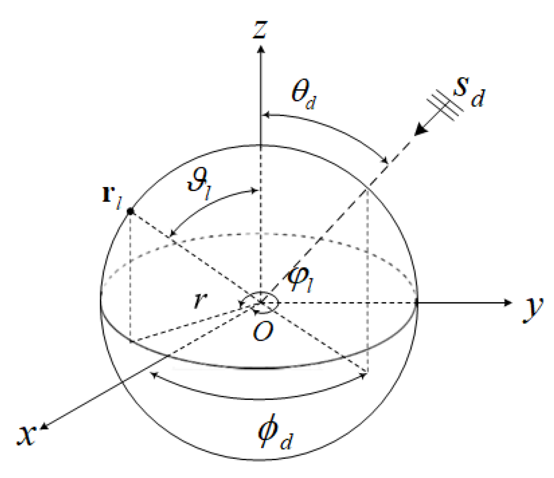
2. Data Model
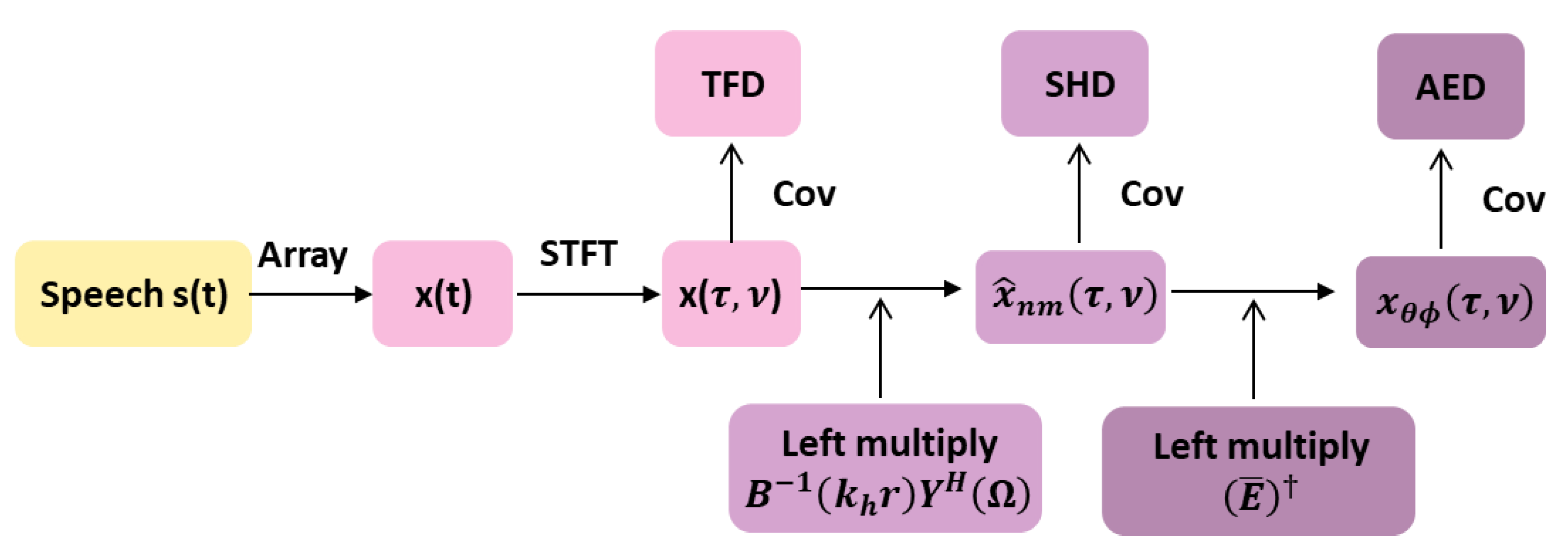
3. The Proposed Method
3.1. TFD Matrix
3.2. SHD Matrix
3.3. AED Matrix
| Algorithm 1 The algorithm of proposed input features |
| Input: received signal x(t) Output: TFD, SHD, AED |
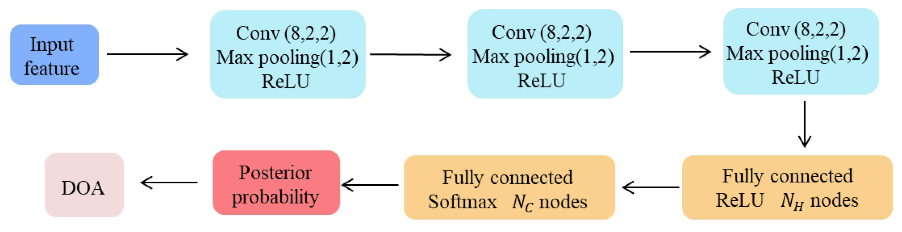
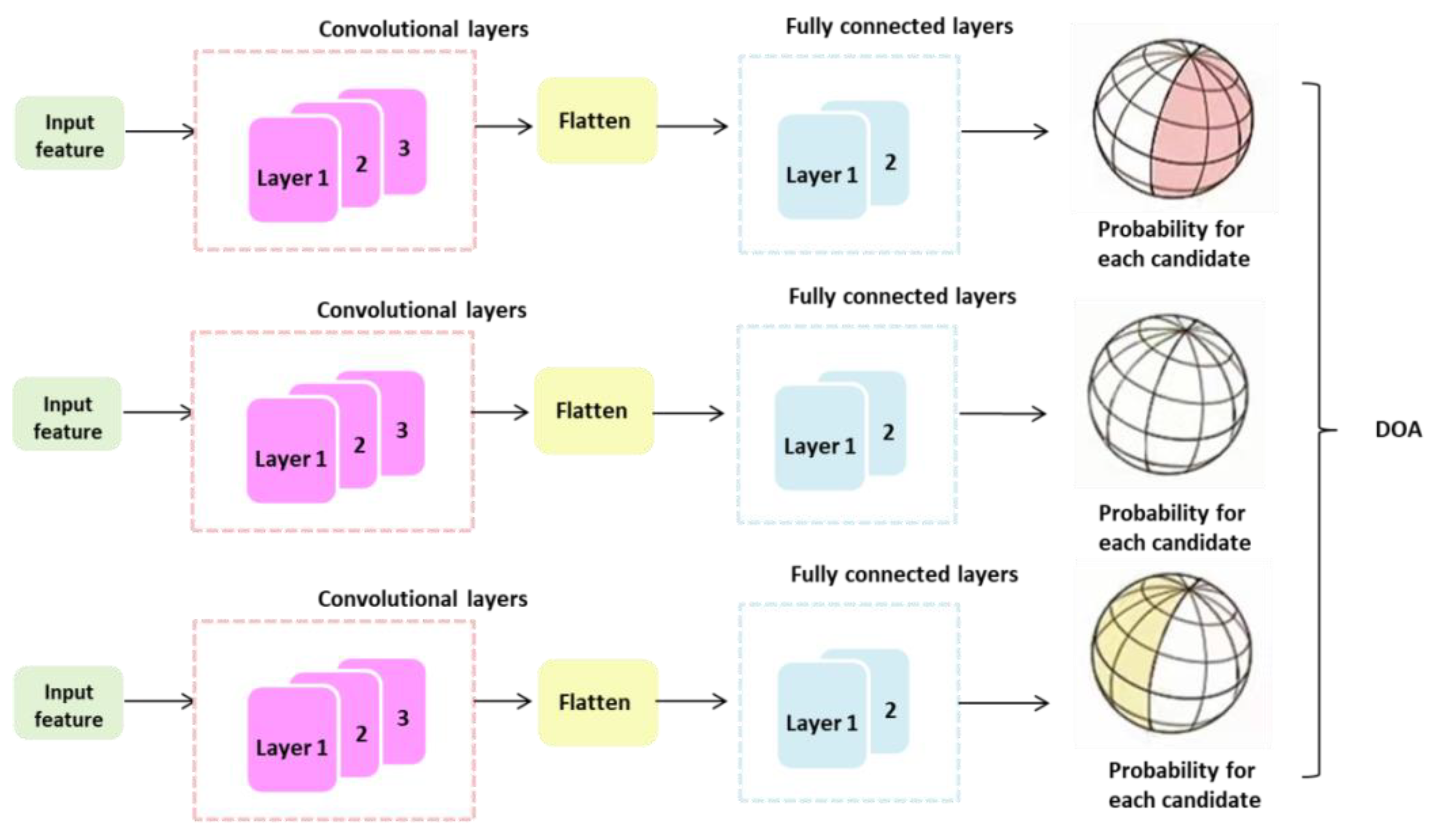
4. Learning Strategies and Network Architectures
4.1. Regular Strategy
4.2. Segmentation Strategy
5. Simulations and Evaluation
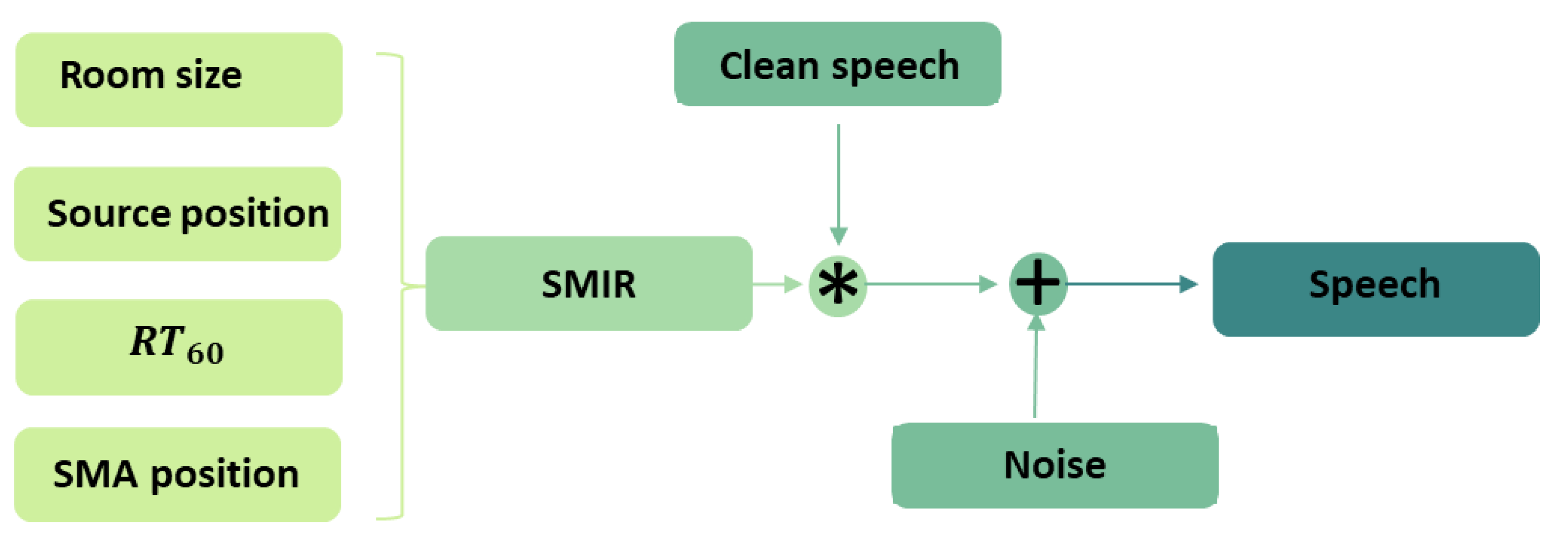
5.1. Dataset
5.1.1. Training Dataset
5.1.2. Testing Dataset
5.2. Methods for Comparison
5.2.1. SH-MUSIC
5.2.2. DPD-MUSIC
5.2.3. FOA
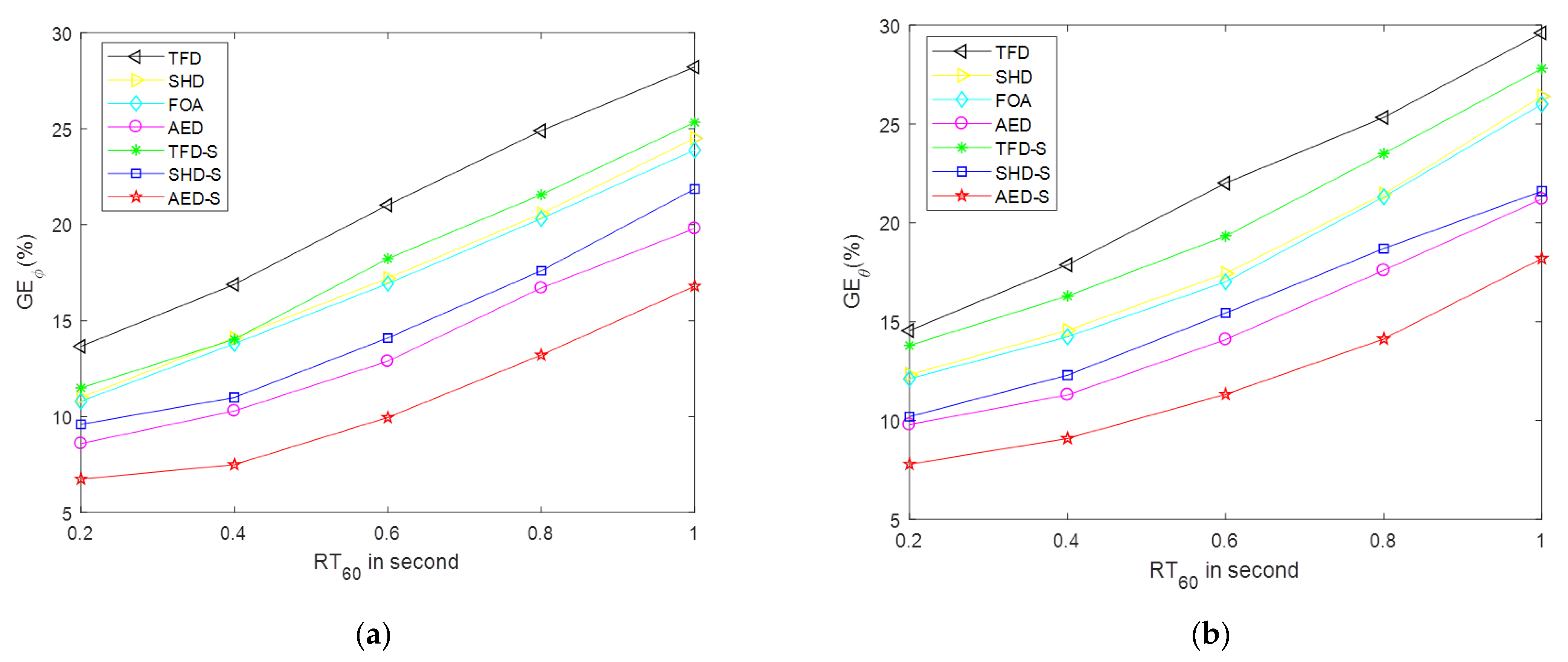
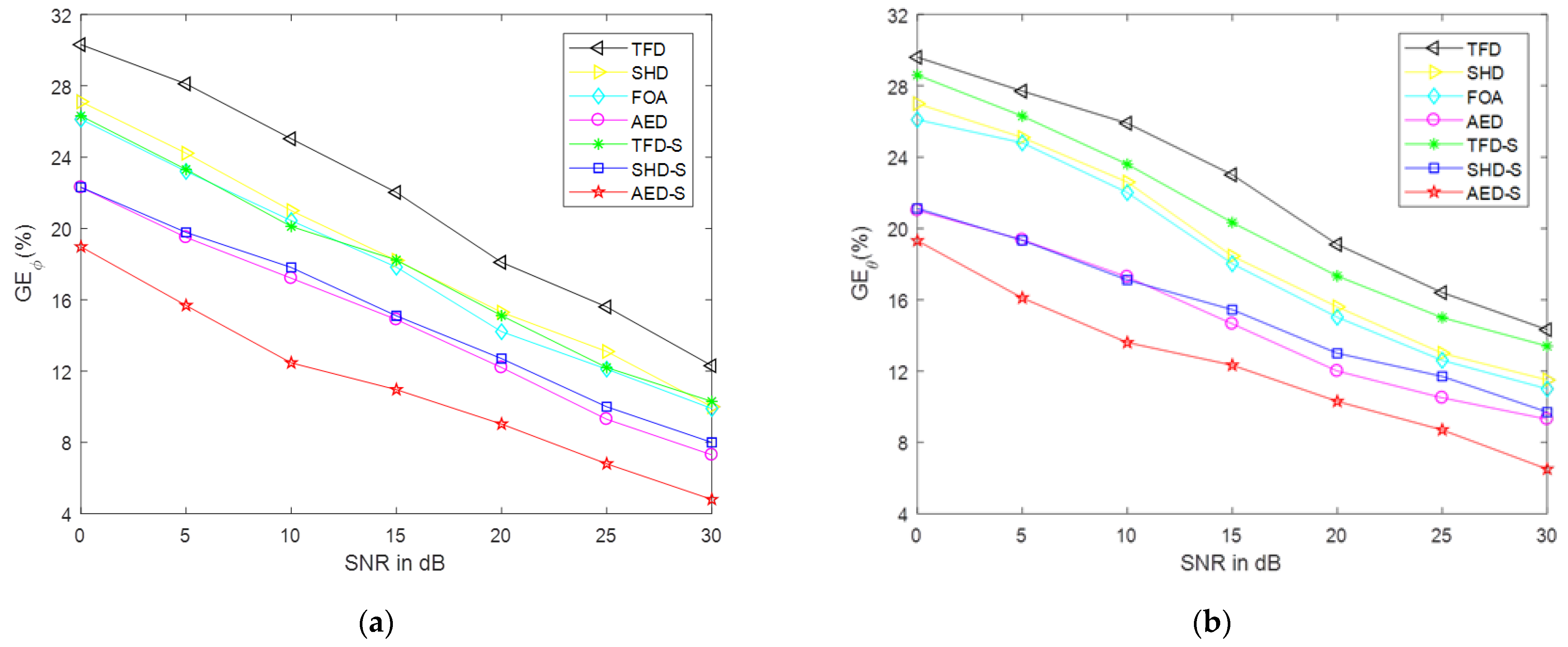
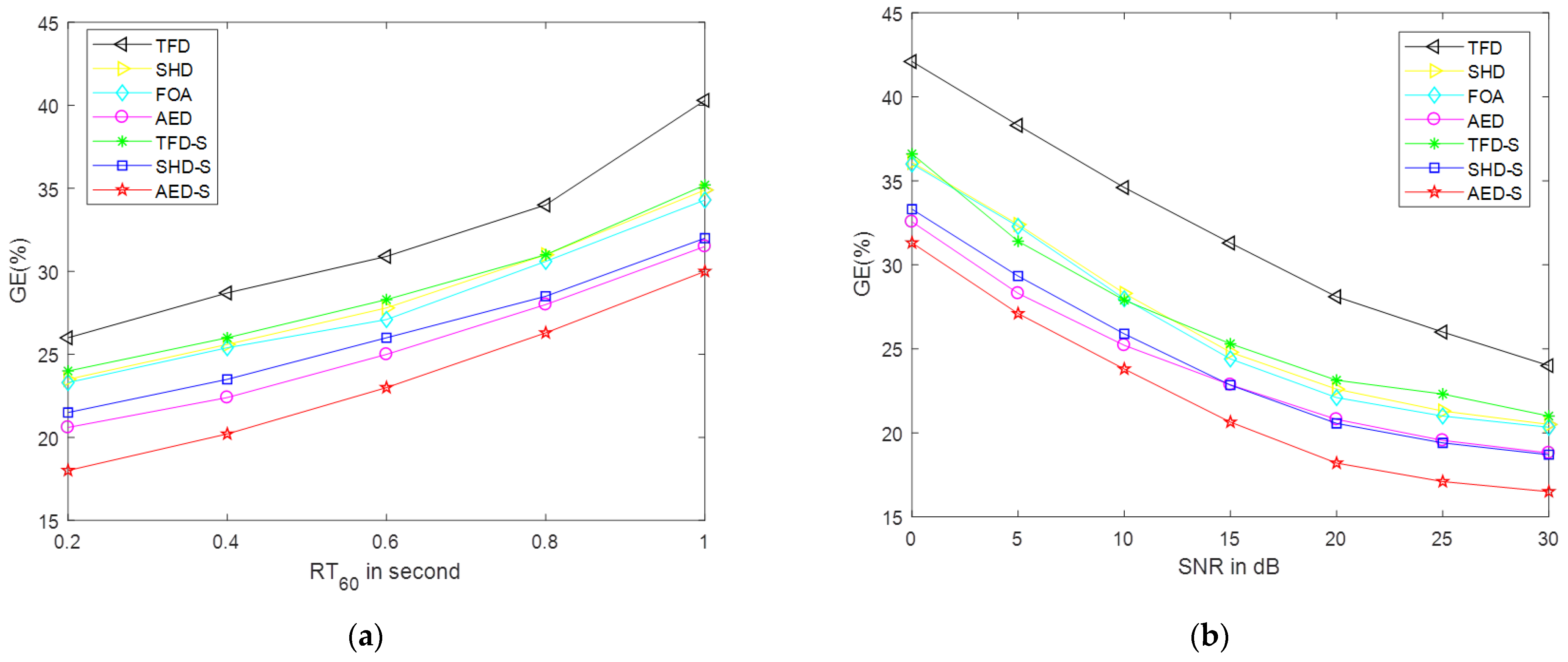
5.3. Measure
5.4. Results in the Real Dataset
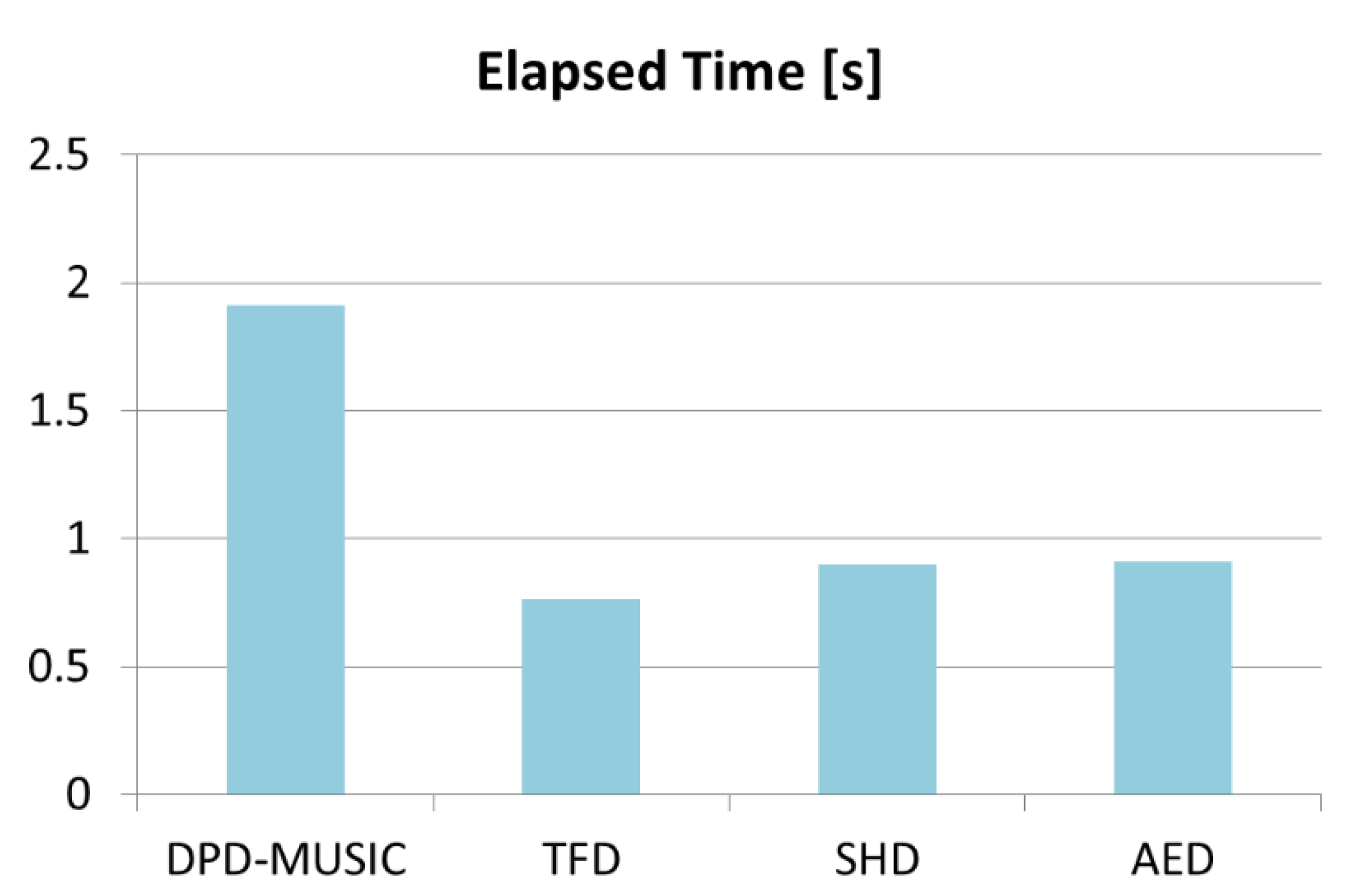
6. Computational Complexity
6.1. DPD-MUSIC
6.2. Proposed Method
6.3. Elapsed Time Comparison
7. Conclusions
Author Contributions
Funding
Institutional Review Board Statement
Informed Consent Statement
Data Availability Statement
Conflicts of Interest
References
- Knight, W.C.; Pridham, R.G.; Kay, S.M. Digital signal processing for sonar. Proc. IEEE 1981, 69, 1451–1506. [Google Scholar] [CrossRef]
- Boukerche, A.; Oliveira, H.A.B.F.; Nakamura, E.F.; Loureiro, A.A.F. Localization systems for wireless sensor networks. IEEE Wirel. Commun. 2007, 14, 6–12. [Google Scholar] [CrossRef]
- Krim, H.; Viberg, M. Two decades of array signal processing research: The parametric approach. IEEE Signal Process. Mag. 1996, 13, 67–94. [Google Scholar] [CrossRef]
- Gannot, S.; Vincent, E.; Markovich-Golan, S.; Ozerov, A. A Consolidated Perspective on Multimicrophone Speech Enhancement and Source Separation. IEEE/ACM Trans. Audio Speech Lang. Process. 2017, 25, 692–730. [Google Scholar] [CrossRef] [Green Version]
- Wang, H.; Chu, P. Voice source localization for automatic camera pointing system in videoconferencing. In Proceedings of the 1997 IEEE International Conference on Acoustics, Speech, and Signal Processing, Munich, Germany, 21–24 April 1997; Volume 1, pp. 187–190. [Google Scholar]
- Yu, Y.; Wang, W.; Luo, J.; Feng, P. Localization based stereo speech separation using deep networks. In Proceedings of the 2015 IEEE International Conference on Digital Signal Processing (DSP), Singapore, 21–24 July 2015; pp. 153–157. [Google Scholar]
- Schmidt, R. Multiple emitter location and signal parameter estimation. IEEE Trans. Antennas Propag. 1986, 34, 276–280. [Google Scholar] [CrossRef] [Green Version]
- Roy, R.; Kailath, T. ESPRIT-estimation of signal parameters via rotational invariance techniques. IEEE Trans. Acoust. Speech Signal Process. 1989, 37, 984–995. [Google Scholar] [CrossRef] [Green Version]
- Capon, J. High-resolution frequency-wavenumber spectrum analysis. Proc. IEEE 1969, 57, 1408–1418. [Google Scholar] [CrossRef] [Green Version]
- Yang, J.-M.; Lee, C.-H.; Kim, S.; Kang, H.-G. A robust time difference of arrival estimator in reverberant environments. In Proceedings of the 2009 17th European Signal Processing Conference, Glasgow, Scotland, 24–28 August 2009; pp. 864–868. [Google Scholar]
- Knapp, C.; Carter, G. The generalized correlation method for estimation of time delay. IEEE Trans. Acoust. Speech Signal Process. 1976, 24, 320–327. [Google Scholar] [CrossRef] [Green Version]
- Lemos, R.P.; e Silva, H.V.L.; Flores, E.L.; Kunzler, J.A.; Burgos, D.F. Spatial Filtering Based on Differential Spectrum for Improving ML DOA Estimation Performance. IEEE Signal Process. Lett. 2016, 23, 1811–1815. [Google Scholar] [CrossRef]
- Huang, Z.; Xu, J.; Pan, J. A Regression Approach to Speech Source Localization Exploiting Deep Neural Network. In Proceedings of the 2018 IEEE Fourth International Conference on Multimedia Big Data (BigMM), Xi’an, China, 13–16 September 2018; pp. 1–6. [Google Scholar]
- Zhu, W.; Zhang, M. A Deep Learning Architecture for Broadband DOA Estimation. In Proceedings of the 2019 IEEE 19th International Conference on Communication Technology (ICCT), Xi’an, China, 16–19 October 2019; pp. 244–247. [Google Scholar]
- Zhu, W.; Zhang, M.; Li, P.; Wu, C. Two-Dimensional DOA Estimation via Deep Ensemble Learning. IEEE Access 2020, 8, 124544–124552. [Google Scholar] [CrossRef]
- Diaz-Guerra, D.; Miguel, A.; Beltran, J.R. Robust Sound Source Tracking Using SRP-PHAT and 3D Convolutional Neural Networks. IEEE/ACM Trans. Audio Speech Lang. Process. 2021, 29, 300–311. [Google Scholar] [CrossRef]
- Shimada, K.; Koyama, Y.; Takahashi, N.; Takahashi, S.; Mitsufuji, Y. Accdoa: Activity-Coupled Cartesian Direction of Arrival Representation for Sound Event Localization and Detection. In Proceedings of the ICASSP 2021—2021 IEEE International Conference on Acoustics, Speech and Signal Processing (ICASSP), Toronto, ON, Canada, 6–11 June 2021; pp. 915–919. [Google Scholar]
- Xiao, X.; Zhao, S.; Zhong, X.; Jones, D.L.; Chng, E.S.; Li, H. A learning based approach to direction of arrival estimation in noisy and reverberantenvironments. In Proceedings of the 2015 IEEE International Conference on Acoustics, Speech and Signal Processing (ICASSP), South Brisbane, QLD, Australia, 19–24 April 2015; pp. 2814–2818. [Google Scholar]
- Stöter, F.; Chakrabarty, S.; Edler, B.; Habets, E.A.P. Classification vs. Regression in Supervised Learning for Single Channel Speaker Count Estimation . In Proceedings of the 2018 IEEE International Conference on Acoustics, Speech and Signal Processing (ICASSP), Calgary, AB, Canada, 15–20 April 2018; pp. 436–440. [Google Scholar]
- Perotin, L.; Défossez, A.; Vincent, E.; Serizel, R.; Guérin, A. Regression Versus Classification for Neural Network Based Audio Source Localization. In Proceedings of the 2019 IEEE Workshop on Applications of Signal Processing to Audio and Acoustics (WASPAA), New Paltz, NY, USA, 20–23 October 2019; pp. 343–347. [Google Scholar]
- Varanasi, V.; Gupta, H.; Hegde, R.M. A Deep Learning Framework for Robust DOA Estimation Using Spherical Harmonic Decomposition. IEEE/ACM Trans. Audio Speech Lang. Process. 2020, 28, 1248–1259. [Google Scholar] [CrossRef]
- Chakrabarty, S.; Habets, E.A.P. Broadband DOA estimation using convolutional neural networks trained with noise signals. In Proceedings of the 2017 IEEE Workshop on Applications of Signal Processing to Audio and Acoustics (WASPAA), New Paltz, NY, USA, 15–18 October 2017. [Google Scholar]
- Adavanne, S.; Politis, A.; Virtanen, T. Sound Event Localization and Detection of Overlapping Sources Using Convolutional Recurrent Neural Networks. IEEE J. Sel. Top. Signal Process. 2018, 13, 34–48. [Google Scholar] [CrossRef] [Green Version]
- Liu, Z.; Zhang, C.; Yu, P.S. Direction-of-Arrival Estimation Based on Deep Neural Networks with Robustness to Array Imperfections. IEEE Trans. Antennas Propag. 2018, 66, 7315–7327. [Google Scholar] [CrossRef]
- Perotin, L.; Serizel, R.; Vincent, E.; Guérin, A. CRNN-based Joint Azimuth and Elevation Localization with the Ambisonics Intensity Vector. In Proceedings of the 2018 16th International Workshop on Acoustic Signal Enhancement (IWAENC), Tokyo, Japan, 17–20 September 2018. [Google Scholar]
- Rafaely, B. Analysis and design of spherical microphone arrays. IEEE Trans. Speech Audio Process. 2005, 13, 135–143. [Google Scholar] [CrossRef]
- Avargel, Y.; Cohen, I. On multiplicative transfer function approximationin the short-time fourier transform domain. IEEE Signal Process. Lett. 2007, 14, 337–340. [Google Scholar] [CrossRef]
- Nadiri, O.; Rafaely, B. Localization of multiple speakers under high reverberation using a spherical microphone array and the direct-pathdominance test. IEEE Trans. Audio Speech Lang. Process. 2014, 22, 1494–1505. [Google Scholar] [CrossRef]
- Rafaely, B. Plane-wave decomposition of the pressure on a sphere by spherical convolution. J. Acoust. Soc. Am. 2004, 116, 2149–2157. [Google Scholar] [CrossRef] [Green Version]
- Paulraj, A.; Roy, R.; Kailath, T. Estimation of signal parameters via rotational invariance techniques-esprit. In Proceedings of the Nineteeth Asilomar Conference on Circuits, Systems and Computers, Pacific Grove, CA, USA, 6–8 November 1985; Volume 37, pp. 83–89. [Google Scholar]
- Huang, Q.; Chen, T. One-Dimensional MUSIC-Type Algorithm for Spherical Microphone Arrays. IEEE Access 2020, 8, 28178–28187. [Google Scholar] [CrossRef]
- Krizhevsky, A.; Sutskever, I.; Hinton, G.E. Imagenet classification with deep convolutional neural networks. Adv. Neural Inf. Process. Syst. 2012, 25, 1097–1105. [Google Scholar] [CrossRef]
- Wang, C.; Xu, Q.; Li, X.; Zheng, G.; Liu, B.; Cheng, Y. An Objective Technique for Typhoon Monitoring with Satellite Infrared Imagery. In Proceedings of the 2019 Photonics & Electromagnetics Research Symposium-Fall (PIERS-Fall), Xiamen, China, 17–20 December 2019; pp. 3218–3221. [Google Scholar]
- Singh, P.P.; Kaushik, R.; Singh, H.; Kumar, N.; Rana, P.S. Convolutional Neural Networks Based Plant Leaf Diseases Detection Scheme. In Proceedings of the 2019 IEEE Globecom Workshops (GC Wkshps), Waikoloa, HI, USA, 9–13 December 2019; pp. 1–7. [Google Scholar]
- Kingma, D.P.; Ba, J. Adam: A method for stochastic optimization. In Proceedings of the 3rd International Conference for Learning Representations, ICLR 2015, San Diego, CA, USA, 7–9 May 2015. [Google Scholar]
- Jarrett, D.P.; Habets, E.A.P.; Thomas, M.R.P.; Naylor, P.A. Rigidsphere room impulse response simulation: Algorithm and applications. J. Acoust. Soc. Am. 2012, 132, 1462–1472. [Google Scholar] [CrossRef] [PubMed] [Green Version]
- The Eigenmike Microphone Array. 2013. Available online: http://www.mhacoustics.com/ (accessed on 3 April 2022).
- Speech activity detection and enhancement of a moving speaker based on the wideband generalized likelihood ratio and microphone arrays. J. Acoust. Soc. Am. 2004, 116, 2406–2415. [CrossRef] [PubMed]
- Varzandeh, R.; Adiloğlu, K.; Doclo, S.; Hohmann, V. Exploiting Periodicity Features for Joint Detection and DOA Estimation of Speech Sources Using Convolutional Neural Networks. In Proceedings of the ICASSP 2020—2020 IEEE International Conference on Acoustics, Speech and Signal Processing (ICASSP), Barcelona, Spain, 4–8 May 2020; pp. 566–570. [Google Scholar]
- Panayotov, V.; Chen, G.; Povey, D.; Khudanpur, S. Librispeech: An ASR corpus based on public domain audio books. In Proceedings of the 2015 IEEE International Conference on Acoustics, Speech and Signal Processing (ICASSP), South Brisbane, QLD, Australia, 19–24 April 2015; pp. 5206–5210. [Google Scholar]
- Evers, C.; Löllmann, H.W.; Mellmann, H.; Schmidt, A.; Barfuss, H.; Naylor, P.A.; Kellermann, W. The LOCATA Challenge: Acoustic Source Localization and Tracking. IEEE/ACM Trans. Audio Speech Lang. Process. 2020, 28, 1620–1643. [Google Scholar] [CrossRef]
- Kumar, L.; Bi, G.; Hegde, R.M. The spherical harmonics root-music. In Proceedings of the 2016 IEEE International Conference on Acoustics, Speech and Signal Processing (ICASSP), Shanghai, China, 20–25 March 2016; pp. 3046–3050. [Google Scholar]
- Rafaely, B.; Kolossa, D. Speaker localization in reverberant rooms based on direct path dominance test statistics. In Proceedings of the 2017 IEEE International Conference on Acoustics, Speech and Signal Processing (ICASSP), New Orleans, LA, USA, 5–9 March 2017; pp. 6120–6124. [Google Scholar]
- Tang, Z.; Kanu, J.D.; Hogan, K.; Manocha, D. Regression and Classification for Direction-of-Arrival Estimation with Convolutional Recurrent Neural Networks. arXiv 2019, arXiv:1904.08452. [Google Scholar]
- Pei, S.; Chang, J.; Ding, J.; Chen, M. Eigenvalues and Singular Value Decompositions of Reduced Biquaternion Matrices. IEEE Trans. Circuits Syst. I Regul. Pap. 2008, 55, 2673–2685. [Google Scholar]
- Rubsamen, M.; Gershman, A.B. Direction-of-arrival estimation for nonuniform sensor arrays: From manifold separation to fourier domain music methods. IEEE Trans. Signal Process. 2009, 57, 588–599. [Google Scholar] [CrossRef]
- Cheng, Y.; Yu, F.X.; Feris, R.S.; Kumar, S.; Choudhary, A.; Chang, S.-F. An exploration of parameter redundancy in deep networks with circulant projections. In Proceedings of the IEEE International Conference on Computer Vision (ICCV), Santiago, Chile, 7–13 December 2015; pp. 2857–2865. [Google Scholar]


| TFD | SHD | AED | |
|---|---|---|---|
| Dimension |
| Parameter | Training Stage | Testing Stage |
|---|---|---|
| DOA | θ: step-10°; ϕ: step-10° | Randomly |
| SNR | Randomly | step-5dB |
| Randomly | step-0.2s | |
| Speech | Librispeech Dev | Librispeech Test |
| Noise | White Gaussian Noise | White Gaussian Noise |
| Room | Room 1–4 | Room 1–6 |
| Method | |||
|---|---|---|---|
| MUSIC | 52.68% | 65.02% | 74.56% |
| DPD-MUSIC | 38.77% | 41.77% | 44.34% |
| FOA | 16.77% | 23.96% | 28.01% |
| TFD | 21.56% | 26.67% | 30.45% |
| TFD-S | 18.23% | 24.63% | 27.89% |
| SHD | 16.98% | 23.63% | 28.77% |
| SHD-S | 14.84% | 19.62% | 25.33% |
| AED | 13.05% | 18.08% | 25.08% |
| AED-S | 9.96% | 14.77% | 21.86% |
| Method | |||
|---|---|---|---|
| MUSIC | 51.56% | 63.46% | 72.41% |
| DPD-MUSIC | 36.41% | 38.55% | 45.06% |
| FOA | 18.24% | 24.01% | 28.96% |
| TFD | 22.01% | 27.78% | 31.30% |
| TFD-S | 19.33% | 26.45% | 29.41% |
| SHD | 18.02% | 23.88% | 28.46% |
| SHD-S | 16.63% | 20.31% | 27.13% |
| AED | 13.43% | 19.27% | 26.11% |
| AED-S | 11.33% | 17.31% | 25.05% |
| Method | Mean Deviation | Standard Deviation |
|---|---|---|
| FOA | ||
| TFD | ||
| TFD-S | ||
| SHD | ||
| SHD-S | ||
| AED | ||
| AED-S |
Publisher’s Note: MDPI stays neutral with regard to jurisdictional claims in published maps and institutional affiliations. |
© 2022 by the authors. Licensee MDPI, Basel, Switzerland. This article is an open access article distributed under the terms and conditions of the Creative Commons Attribution (CC BY) license (https://creativecommons.org/licenses/by/4.0/).
Share and Cite
Huang, Q.; Fang, W. A Deep Learning Method for DOA Estimation with Covariance Matrices in Reverberant Environments. Appl. Sci. 2022, 12, 4278. https://doi.org/10.3390/app12094278
Huang Q, Fang W. A Deep Learning Method for DOA Estimation with Covariance Matrices in Reverberant Environments. Applied Sciences. 2022; 12(9):4278. https://doi.org/10.3390/app12094278
Chicago/Turabian StyleHuang, Qinghua, and Weilun Fang. 2022. "A Deep Learning Method for DOA Estimation with Covariance Matrices in Reverberant Environments" Applied Sciences 12, no. 9: 4278. https://doi.org/10.3390/app12094278