
3-D Sound Image Reproduction Method Based on Spherical Harmonic Expansion for 22.2 Multichannel Audio


Abstract
:1. Introduction
- 1.
- The arrival of sound from all directions surrounding a listening position;
- 2.
- High quality 3-D sound impression beyond the 5.1 multichannel audio;
- 3.
- High accuracy adjustment of the position between sound and video images.
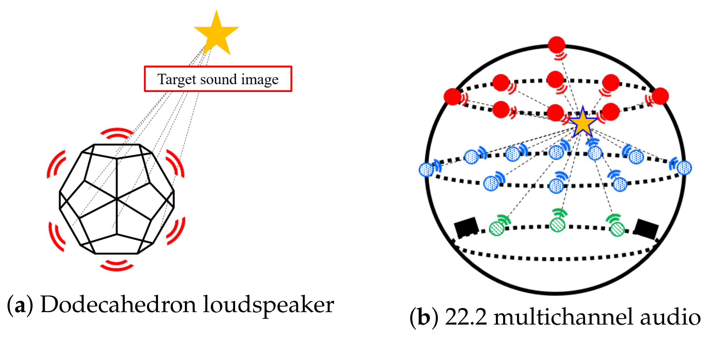
2. Conventional 3-D Sound Image Reproduction Based on VBAP
- 1.
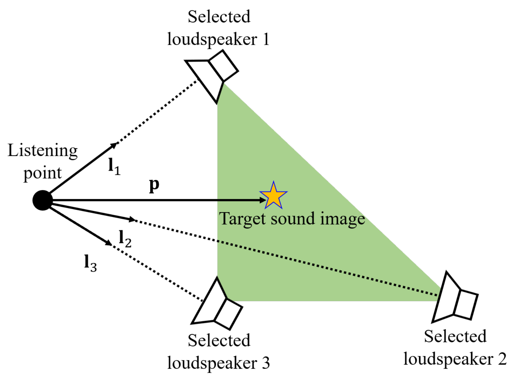
- Obtaining the 3-D sound source position vector .Panning requires the position vector of the 3-D sound image to generate signals for reproduction of the sound image. The vector is acquired automatically or manually from media such as video.
- 2.
- Calculation of the gain vector .VBAP calculates the gain vector to control the sound image by using and each unit vector , , from the listening point to the three loudspeakers. In VBAP, it is assumed that the 3-D sound image is on the median point among the three loudspeakers. Hence, the position of the 3-D sound image is represented as:where is the matrix of unit vectors. From Equation (1), the gain vector is obtained by:
- 3.
- Normalize the gain vector .To prevent excessive sound pressure, the gain vector should be normalized by the norm as:where is the normalized gain vector.
- 4.
- Generation of the input signals of the three loudspeakers.The input signals are generated by the object signal and the calculated gains , , and as:where t is the time index and is the loudspeaker index.
3. Proposed 3-D Sound Image Reproduction Based on Spherical Harmonic Expansion
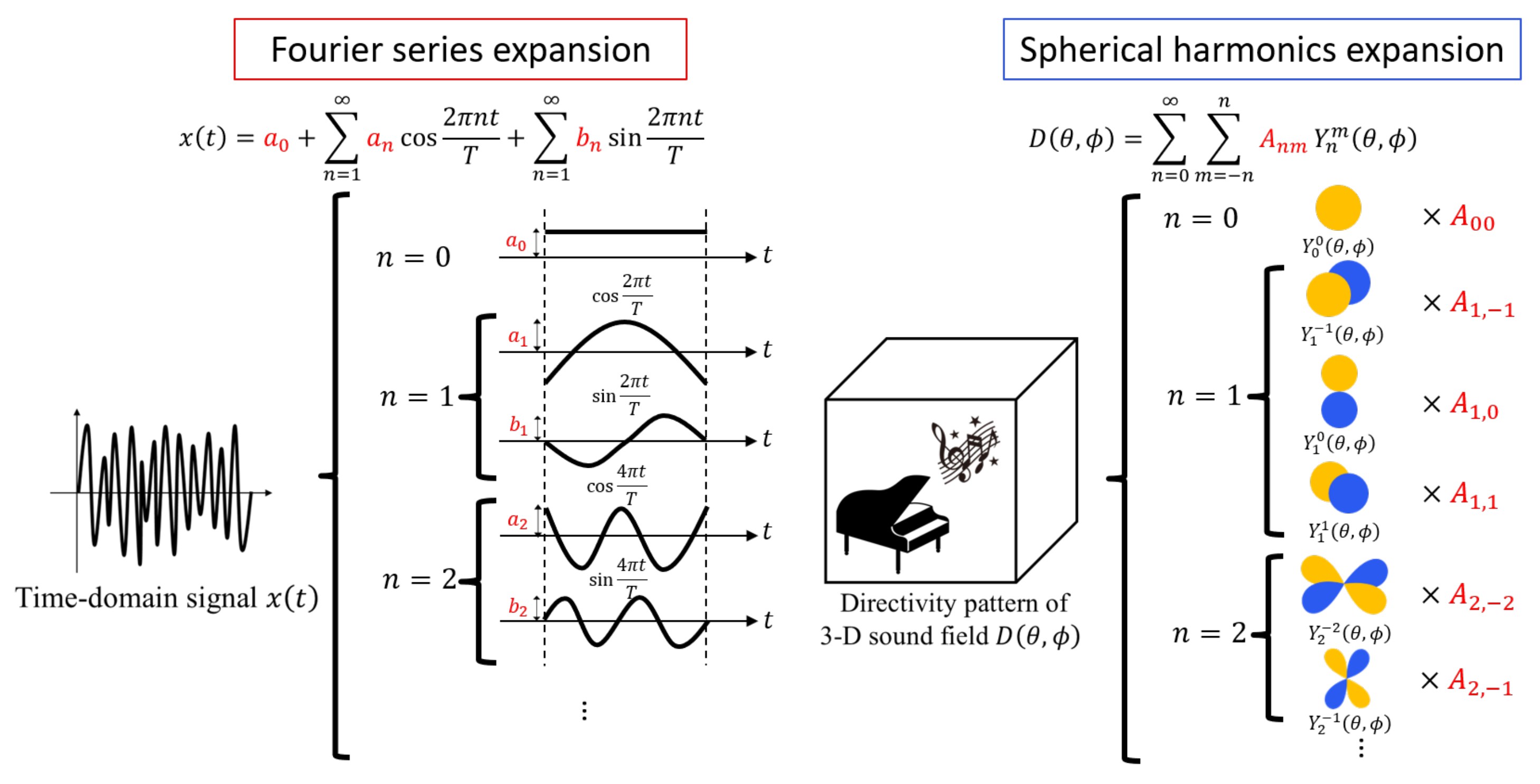
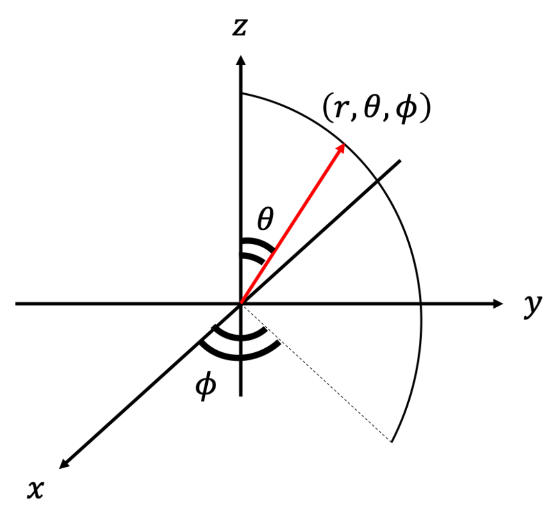
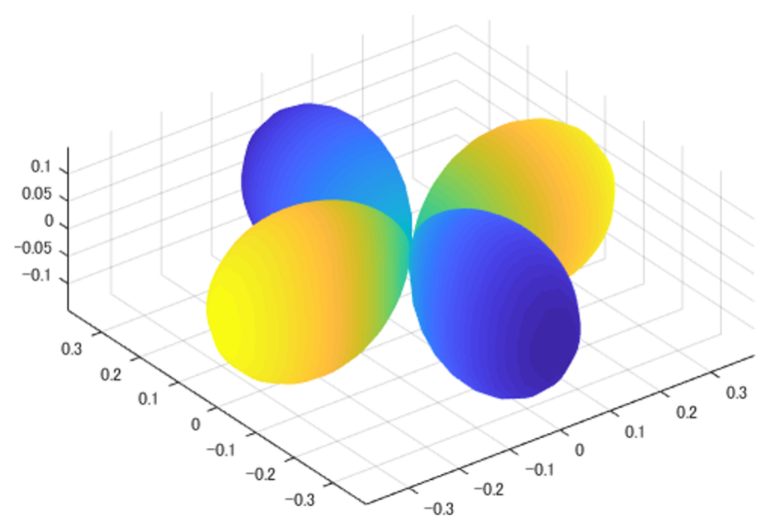
3.1. Spherical Harmonic Expansion
3.2. Algorithm of Proposed Method
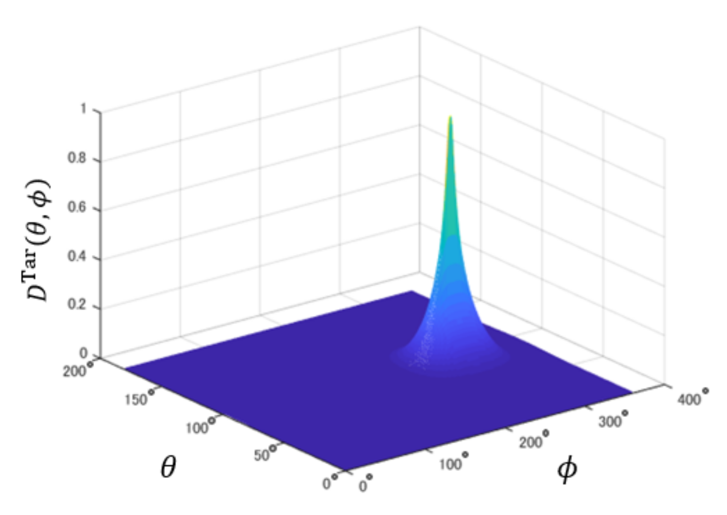
- 1.
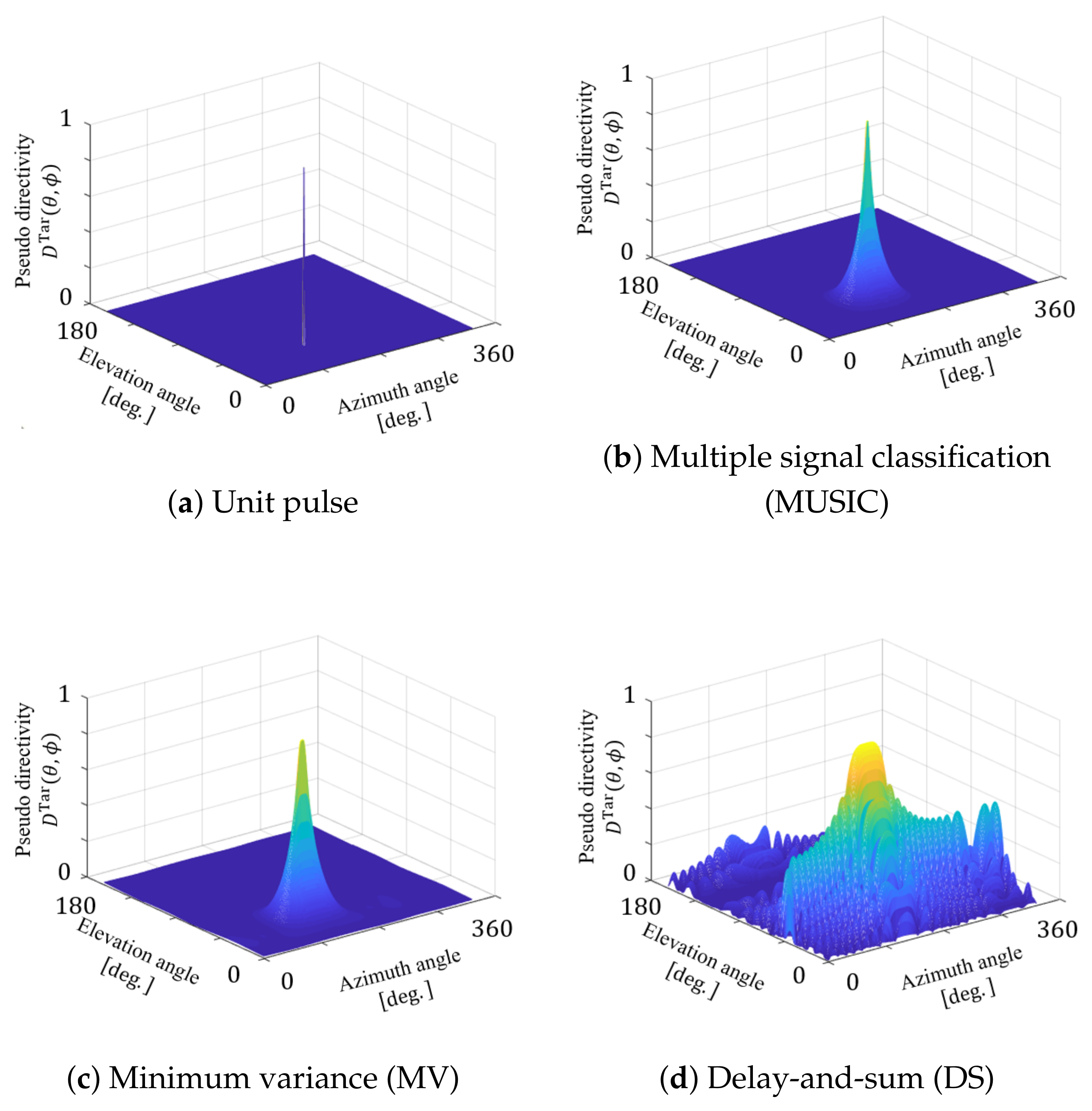
- Generation of a target directivity pattern .The proposed method requires a target directivity pattern including a peak at the target sound image position. This directivity pattern affects the clarity of the 3-D sound image at the target position. In this paper, a provisional directivity pattern is generated by multiple signal classification (MUSIC) [16]. MUSIC estimates the direction of arrival of a sound source and generates the sharp spatial spectrum to the direction of the sound source. In Step 1, we generate the spatial spectrum for the target sound image at the position of by using MUSIC. Then, the generated spatial spectrum is normalized to the target directivity pattern as:where is the position with the smallest spatial spectrum. An example of the target directivity pattern is shown in Figure 8.
- 2.
- Calculation of the target directivity pattern in the SH domain .
- 3.
- Calculation of the weighting factor .We calculate the weighting factor for ith loudspeaker at the position of to reproduce the target directivity pattern in the real sound field. The weighting factor is obtained by:where k is the wave number and is the loudspeaker index. On the basis of the mode matching, the target directivity pattern has a relationship between the weighting factor in the SH domain as:where and are the spherical Bessel function and its derivative, respectively, and is the mode strength [17]. The mode strength theoretically represents the radial strength of the directivity. Substituting Equation (11) into Equation (10), the weighting factor can be obtained as follows:
- 4.
- Generation of the input signals for 22 loudspeakers.The weight factor in the spatial domain can be used as the frequency domain filter, that is,where is the angular frequency and c is the speed of sound. Then, the input signal for ith loudspeaker is obtained by:where is the sound source, and represent the inverse discrete time Fourier transform and discrete time Fourier transform operators, respectively.
4. Evaluation Experiment
4.1. Experiment 1: Evaluation of Sound Image Localization Accuracy
- 1.
- Calculation of inter-aural level difference (ILD) and inter-aural phase difference (IPD)The ILD and IPD were calculated for each recorded sound at positions A to E shown in Table 5 [19]. Here, the ILD and IPD are known as factors for the sound localization of humans. The ILD and IPD can be calculated by:where is the cross spectrum between the signals obtained at the left and right ears of the dummy head microphone, is the power spectrum of the signal obtained at the left ear of the dummy head microphone, and and represent the real and imaginary parts of the complex value, respectively. is the index for the recording position.In addition, and were calculated by using HRTF in the CIPIC database [20]. and represent the value for which the sound image perfectly localizes at the desired position.
- 2.
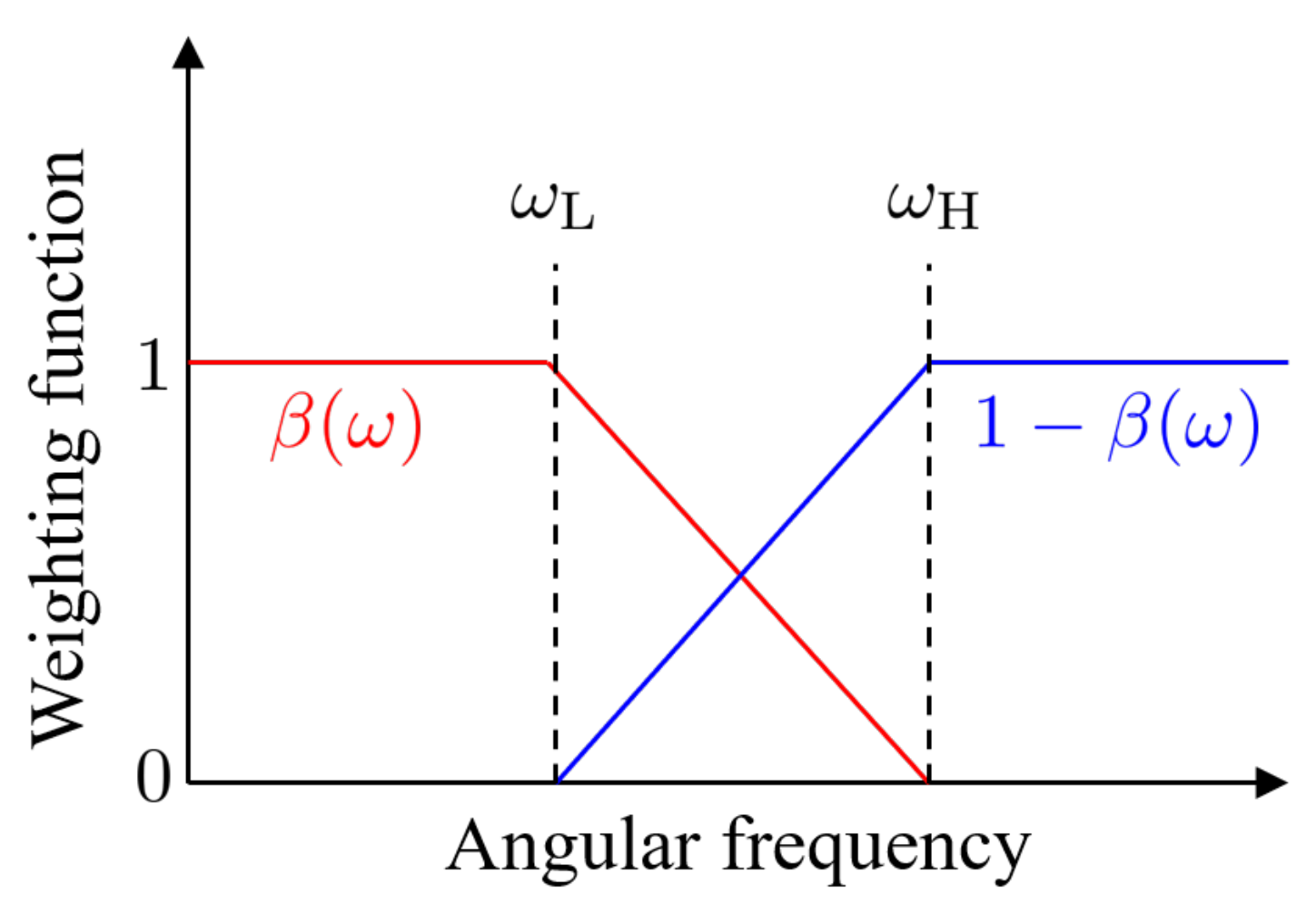
- Calculation of the differences of the ILD and IPD between recorded sound and HRTF database.The differences of the ILD and IPD between the recorded sound and HRTF database were calculated. If the differences are small, it can be said that the sound image localizes at the direction . The difference between the inter-aural time difference (ITD) and IPD are defined as:Then, and were combined as the following form.where is the weighting function that controls the ratio between and in Equation (24). has a characteristic shown in Figure 9. The reason for using is that the IPD affects the sound localization of humans below 1500 Hz and is dominant above 1500 Hz [21]. Hence, we set rad/s and = 12,566 rad/s with consideration of the crossover. These values are related to 1000 and 2000 Hz in terms of frequency. From hereafter, is called the error function.
- 3.
- Estimation of the direction of reconstructed 3-D sound image.The direction of the reconstructed 3-D sound image can be estimated by obtaining of which the error function is the smallest value. Here, the directions of the sound image were estimated for each recorded sound as:where is the highest angular frequency of the recorded sound. In this experiment, the frequency of the sound is up to 8000 Hz and rad/s.
- 4.
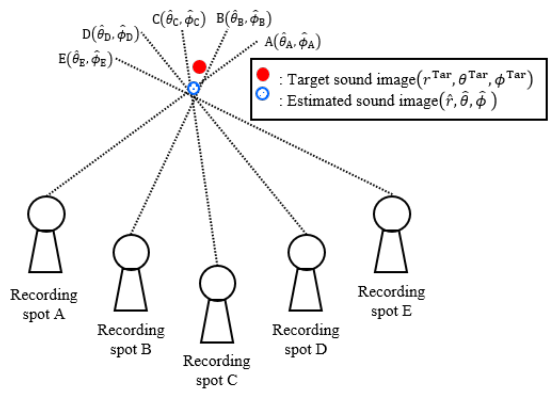
- Estimation of the position of the reconstructed 3-D sound image.Finally, the position of the reconstructed 3-D sound image was estimated by using the estimated direction of the sound image . As shown in Figure 10, the position was estimated by drawing a straight line from each recording position to the estimated direction. Then, the center position of the surrounding area by the five lines was treated as the estimated position of the sound image .
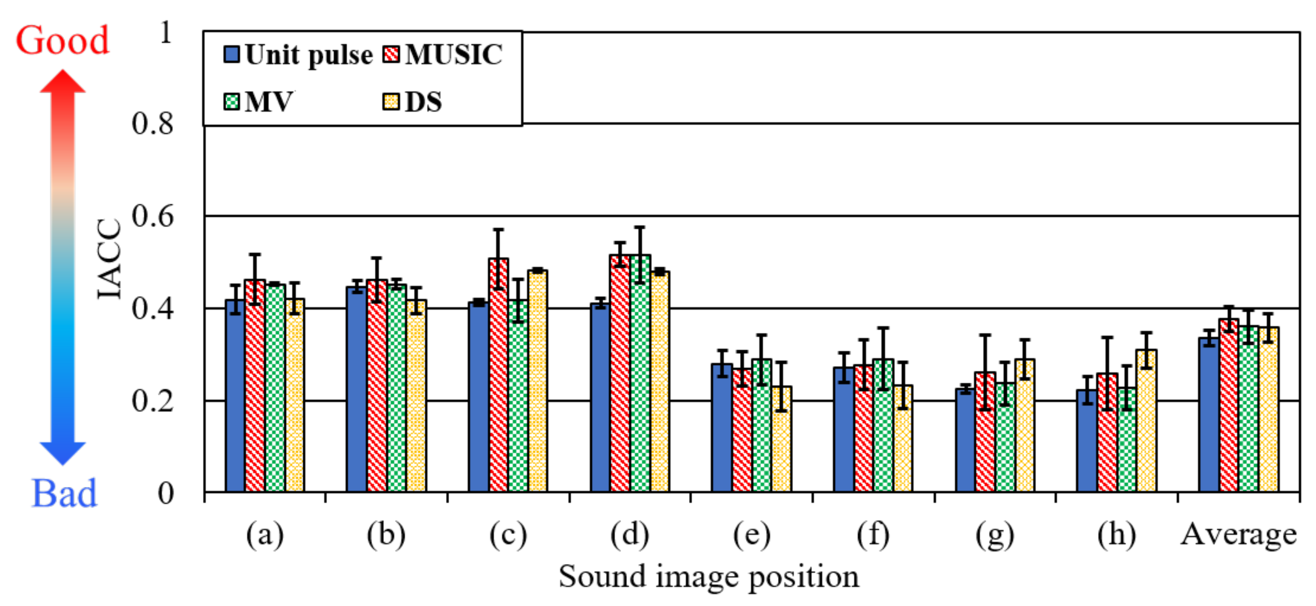
4.2. Experiment 2: Clarity of Reconstructed Sound Image for Given Directivity in Proposed Method
5. Conclusions
Author Contributions
Funding
Institutional Review Board Statement
Informed Consent Statement
Data Availability Statement
Conflicts of Interest
References
- Roginska, A.; Geluso, P. Immersive Sound: The Art and Science of Binaural and Multi-Channel Audio, 1st ed.; Routledge: London, UK, 2017. [Google Scholar]
- Bando, K.; Haneda, Y. Interactive directivity control using dodecahedron loudspeaker array. J. Signal Process. 2016, 20, 209–212. [Google Scholar] [CrossRef] [Green Version]
- Okamoto, T. 2D multizone sound field systhesis with interior-exterior Ambisonics. In Proceedings of the 2021 IEEE Workshop Applications of Signal Processing to Audio and Acoustics, Virtual Event, 18–21 October 2021; pp. 276–280. [Google Scholar]
- Hamasaki, K.; Nishiguchi, T.; Okumura, R.; Nakayama, Y.; Ando, A. A 22.2 Multichannel Sound System for Ultrahigh-Definition TV (UHDTV). SMPTE Motion Imaging J. 2008, 117, 40–49. [Google Scholar] [CrossRef]
- Institutional Telecommunication Union Radiocommunication Sector (ITU-R) Recommendation BS. 2051-2. Advanced Sound System for Programme Production; 2018; Available online: https://www.google.com/url?sa=t&rct=j&q=&esrc=s&source=web&cd=&cad=rja&uact=8&ved=2ahUKEwiIuf-D8_71AhU363MBHQs-CSoQFnoECAMQAQ&url=https%3A%2F%2Fwww.itu.int%2Fdms_pubrec%2Fitu-r%2Frec%2Fbs%2FR-REC-BS.2051-2-201807-I!!PDF-E.pdf&usg=AOvVaw07oyUacd5OYXmikUvzCfj2 (accessed on 20 January 2022).
- Camras, M. Approach to recreating a sound field. J. Acoust. Soc. Am. 1968, 43, 172–178. [Google Scholar] [CrossRef]
- Berkhout, A.J.; de Vries, D.; Vogel, P. Acoustic control by wave field synthesis. J. Acoust. Soc. Am. 1993, 93, 2764–2778. [Google Scholar] [CrossRef]
- Omoto, A.; Ise, S.; Ikeda, Y.; Ueno, K.; Enomoto, S.; Kobayashi, M. Sound field reproduction and sharing system based on the boundary surface control principle. Acoust. Sci. Technol. 2015, 36, 1–11. [Google Scholar] [CrossRef] [Green Version]
- Institutional Telecommunication Union Radiocommunication Sector (ITU-R) Recommendation BS.775-2. Multichannel Stereophonic Sound System with and without Accompanying Picture; 2006; Available online: https://www.google.com/url?sa=t&rct=j&q=&esrc=s&source=web&cd=&ved=2ahUKEwiYg_y58_71AhXY5nMBHeGGBtEQFnoECAUQAQ&url=https%3A%2F%2Fwww.itu.int%2Fdms_pub%2Fitu-r%2Fopb%2Frec%2FR-REC-LS-2007-E02-PDF-E.pdf&usg=AOvVaw3YzFGDUR8es0kBuKwOa9m6 (accessed on 20 January 2022).
- Rumsey, F. Spatial Audio; Focal Press: Waltham, MA, USA, 2001. [Google Scholar]
- Pulkki, V. Virtual Sound Source Positioning Using Vector Base Amplitude Panning. J. Audio Eng. Soc. 1997, 45, 456–466. [Google Scholar]
- Ando, A.; Hamasaki, K. Sound intensity based three-dimensional panning. In Proceedings of the Audio Engineering Society 126th Convention, Munich, Germany, 7–10 May 2009. [Google Scholar]
- Suzuki, H.; Iwai, K.; Nishiura, T. 3-D sound image panning based on spherical harmonics expansion for 22.2 multichannel audio. In Proceedings of the INTER-NOISE 2020, E-Congress, Seoul, Korea, 23–26 August 2020; pp. 4170–4180. [Google Scholar]
- Meyer, J.; Elko, G. A highly scalable spherical microphone array based on an orthonormal decomposition of the soundfield. In Proceedings of the IEEE International Conference on Acoustics, Speech and Signal Processing (ICASSP 2002), Orlando, FL, USA, 13–17 May 2002; pp. II–1781–II–1784. [Google Scholar]
- Müller, C. Spherical Harmonics; Springer: Heidelberg/Berlin, Germany, 2006. [Google Scholar]
- Schmidt, R. Multiple emitter location and signal parameter estimation. IEEE Trans. Antennas Propag. 1986, 34, 276–280. [Google Scholar] [CrossRef] [Green Version]
- Williams, E. Fourier Acoustics: Sound Radiation and Nearfield Acoustical Holography; Springer: Heidelberg/Berlin, Germany, 1999. [Google Scholar]
- Nakashima, H.; Chisaki, Y.; Usagawa, T.; Ebata, M. Frequency domain binaural model based on interaural phase and level differences. Acoust. Sci. Technol. 2003, 24, 172–178. [Google Scholar] [CrossRef] [Green Version]
- Roman, N.; Wang, D.; Brown, G.J. Sound field reproduction and sharing system based on the boundary surface control principle. J. Acoust. Soc. Am. 2003, 114, 2236–2252. [Google Scholar] [CrossRef] [PubMed]
- Algazi, V.R.; Duda, R.O.; Thompson, D.M.; Avendano, C. The CIPIC HRTF Database. In Proceedings of the IEEE Workshop Applications of Signal Processing to Audio and Electroacoustics, Mohonk Mountain House, New Paltz, NY, USA, 21–24 October 2001; pp. 99–102. [Google Scholar]
- Woodworth, R. Experimental Psychology; Holt, Rinehart and Winston: Ballwin, MO, USA, 1938. [Google Scholar]
- Zheng, K.; Otsuka, M.; Nishiura, T. 3-D Sound image localization in reproduction of 22.2 multichannel audio based on room impulse response generation with vector composition. In Proceedings of the International Congress on Acoustics (ICA 2019), Aachen, Germany, 9–13 September 2019; pp. 5274–5281. [Google Scholar]
- Trees, H.L.V. Optimum Array Processing; Wiley: Hoboken, NJ, USA, 2002. [Google Scholar]
- Johnson, D.H.; Dudgeon, D.E. Array Signal Processing; Prentice Hall: Hoboken, NJ, USA, 1993. [Google Scholar]
- Omologo, M.; Svaizer, P. Acoustic event localization using a crosspower-spectrum phase based technique. In Proceedings of the IEEE International Conference on Acoustics, Speech and Signal Processing (ICASSP 1994), Adelaide, SA, Australia, 19–22 April 1994; Volume 2, pp. II/273–II/276. [Google Scholar]


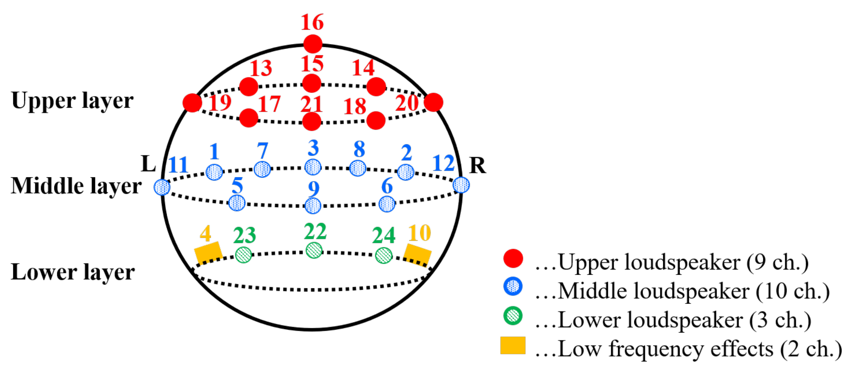
| Layer | Channel No. | Channel Name | Setting Range | |
|---|---|---|---|---|
| Azimuth ( [degs.]) | Elevation ( [degs.]) | |||
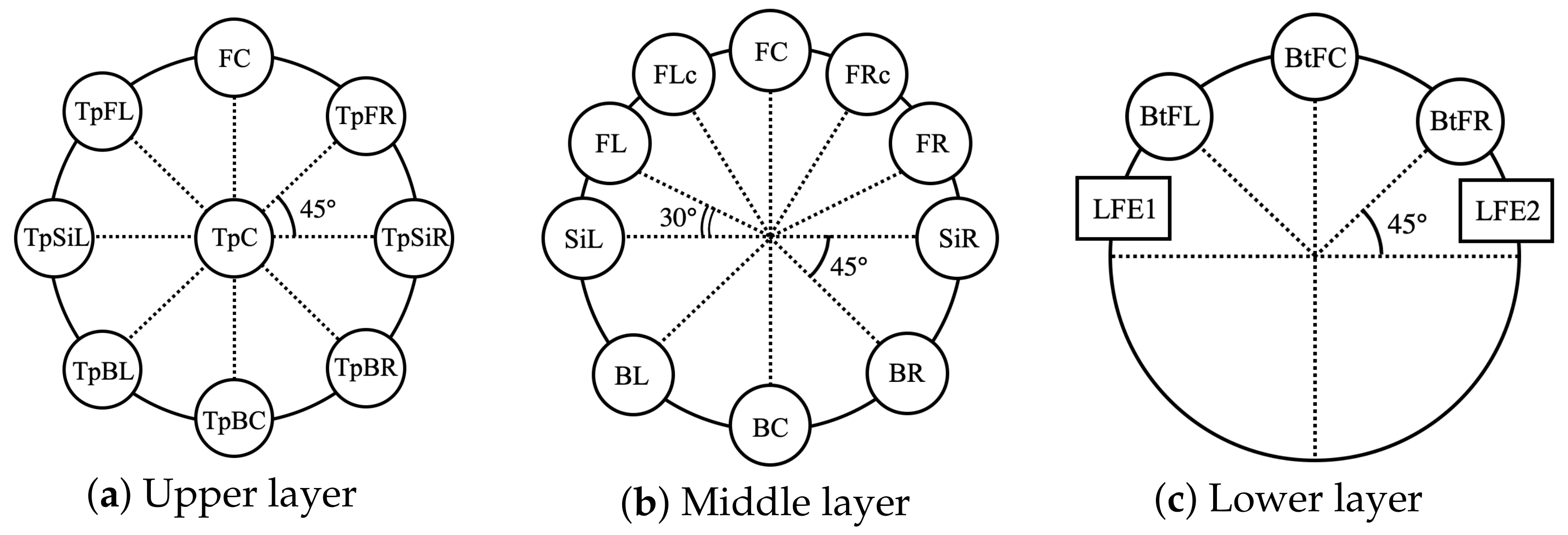
| Middle | 1 | Front left (FL) | 135 ≤ ≤ 150 | 85 ≤ ≤ 90 |
| 2 | Front right (FR) | 30 ≤ ≤ 45 | 85 ≤ ≤ 90 | |
| 3 | Front center (FC) | 90 | 85 ≤ ≤ 90 | |
| Lower | 4 | Low frequency effects-1 | 120 ≤ ≤ 180 | 105 ≤ ≤ 120 |
| Middle | 5 | Back left (BL) | 200 ≤ ≤ 225 | 75 ≤ ≤ 90 |
| 6 | Back right (BR) | 315 ≤ ≤ 340 | 75 ≤ ≤ 90 | |
| 7 | Front left center (FLc) | 112.5 ≤ ≤ 120 | 85 ≤ ≤ 90 | |
| 8 | Front right center (FRc) | 60 ≤ ≤ 67.5 | 85 ≤ ≤ 90 | |
| 9 | Back center (BC) | 270 | 75 ≤ ≤ 90 | |
| Lower | 10 | Low frequency effects-2 | 0 ≤ ≤ 60 | 105 ≤ ≤ 120 |
| Middle | 11 | Side left (SiL) | 180 | 75 ≤ ≤ 90 |
| 12 | Side right (SiR) | 0 | 75 ≤ ≤ 90 | |
| Upper | 13 | Top front left (TpFL) | 135 ≤ ≤ 150 | 45 ≤ ≤ 60 |
| 14 | Top front right (TpFR) | 30 ≤ ≤ 45 | 45 ≤ ≤ 60 | |
| 15 | Top front center (TpFC) | 90 | 45 ≤ ≤ 60 | |
| 16 | Top center (TpC) | N/A | 0 | |
| 17 | Top back left (TpBL) | 200 ≤ ≤ 225 | 45 ≤ ≤ 60 | |
| 18 | Top back right (TpBR) | 315 ≤ ≤ 340 | 45 ≤ ≤ 60 | |
| 19 | Top side left (TpSiL) | 180 | 45 ≤ ≤ 60 | |
| 20 | Top side right (TpSiR) | 0 | 45 ≤ ≤ 60 | |
| 21 | Top back center (TpBC) | 270 | 45 ≤ ≤ 60 | |
| Lower | 22 | Bottom front center (BtFC) | 90 | 105 ≤ ≤ 120 |
| 23 | Bottom front left (BtFL) | 135 ≤ ≤ 150 | 105 ≤ ≤ 120 | |
| 24 | Bottom front right (BtFR) | 30 ≤ ≤ 45 | 105 ≤ ≤ 120 | |
| Environment | Experiment room ( ms) |
| Ambient noise level | 37.0 dBA |
| Sound pressure level | 70.0 dB at the listening point |
| Dummy head | 3Dio, Free Space Pro II |
| Loudspeaker | YAMAHA, VXS5 |
| Loudspeaker (LFE) | YAMAHA, VXS10S |
| Loudspeaker amplifier | YAMAHA, XMV8280 |
| Analog-to-digital converter | RME, Fireface UFX |
| Digital-to-analog converter | RME, M-32 DA |
| Layer | Channel No. | Channel Name | Setting Position | |
|---|---|---|---|---|
| Azimuth ( [degs.]) | Elevation ( [degs.]) | |||
| Middle | 1 | Front left (FL) | 150 | 90 |
| 2 | Front right (FR) | 30 | 90 | |
| 3 | Front center (FC) | 90 | 90 | |
| Lower | 4 | Low frequency effects-1 | 150 | 118.3 |
| Middle | 5 | Back left (BL) | 210 | 90 |
| 6 | Back right (BR) | 330 | 90 | |
| 7 | Front left center (FLc) | 120 | 90 | |
| 8 | Front right center (FRc) | 120 | 90 | |
| 9 | Back center (BC) | 270 | 90 | |
| Lower | 10 | Low frequency effects-2 | 30 | 118.3 |
| Middle | 11 | Side left (SiL) | 180 | 90 |
| 12 | Side right (SiR) | 0 | 90 | |
| Upper | 13 | Top front left (TpFL) | 150 | 52 |
| 14 | Top front right (TpFR) | 30 | 52 | |
| 15 | Top front center (TpFC) | 90 | 52 | |
| 16 | Top center (TpC) | - | 0 | |
| 17 | Top back left (TpBL) | 210 | 52 | |
| 18 | Top back right (TpBR) | 330 | 52 | |
| 19 | Top side left (TpSiL) | 180 | 52 | |
| 20 | Top side right (TpSiR) | 0 | 52 | |
| 21 | Top back center (TpBC) | 270 | 52 | |
| Lower | 22 | Bottom front center (BtFC) | 90 | 118.3 |
| 23 | Bottom front left (BtFL) | 150 | 118.3 | |
| 24 | Bottom front right (BtFR) | 30 | 118.3 | |
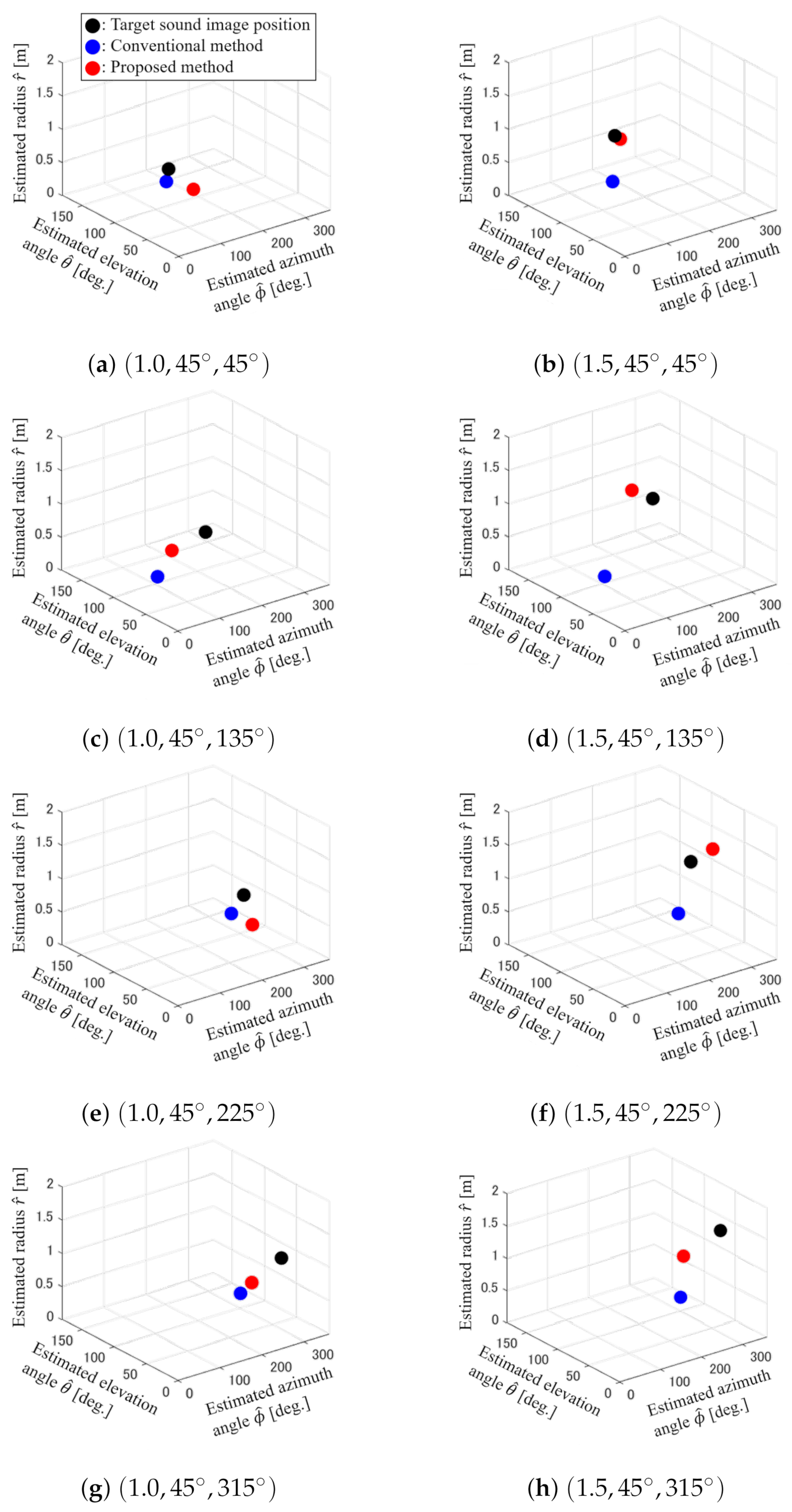
| (a) | |
| (b) | |
| (c) | |
| (d) | |
| (e) | |
| (f) | |
| (g) | |
| (h) |
| A | |
| B | |
| C | |
| D | |
| E |
Publisher’s Note: MDPI stays neutral with regard to jurisdictional claims in published maps and institutional affiliations. |
© 2022 by the authors. Licensee MDPI, Basel, Switzerland. This article is an open access article distributed under the terms and conditions of the Creative Commons Attribution (CC BY) license (https://creativecommons.org/licenses/by/4.0/).
Share and Cite
Iwai, K.; Suzuki, H.; Nishiura, T. 3-D Sound Image Reproduction Method Based on Spherical Harmonic Expansion for 22.2 Multichannel Audio. Appl. Sci. 2022, 12, 1994. https://doi.org/10.3390/app12041994
Iwai K, Suzuki H, Nishiura T. 3-D Sound Image Reproduction Method Based on Spherical Harmonic Expansion for 22.2 Multichannel Audio. Applied Sciences. 2022; 12(4):1994. https://doi.org/10.3390/app12041994
Chicago/Turabian StyleIwai, Kenta, Hiromu Suzuki, and Takanobu Nishiura. 2022. "3-D Sound Image Reproduction Method Based on Spherical Harmonic Expansion for 22.2 Multichannel Audio" Applied Sciences 12, no. 4: 1994. https://doi.org/10.3390/app12041994