
Investigating How Reproducibility and Geometrical Representation in UMAP Dimensionality Reduction Impact the Stratification of Breast Cancer Tumors

 , , ,
, , ,
Abstract
:1. Introduction
2. Materials and Methods
2.1. Data
2.2. UMAP
2.3. Clustering Algorithms
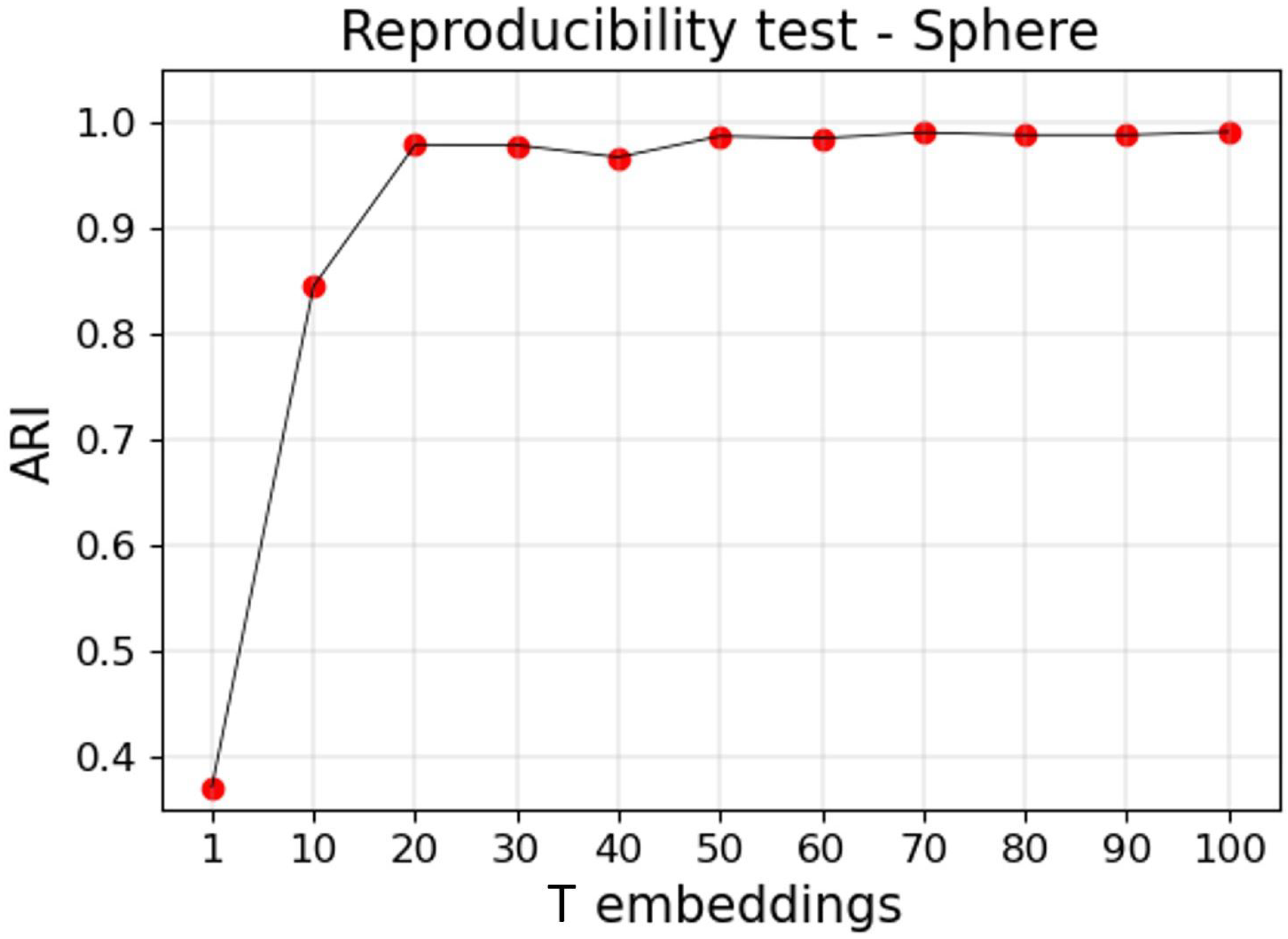
2.4. Reproducibility
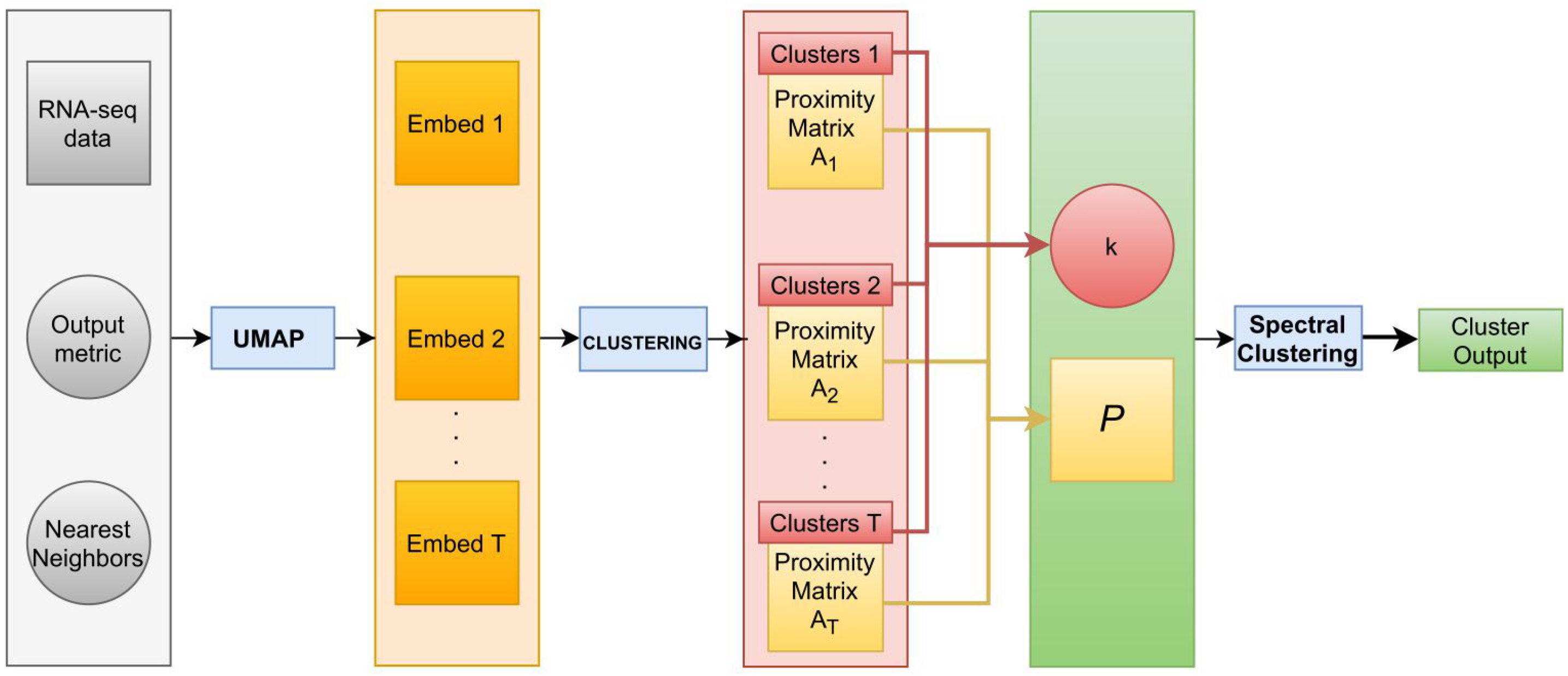
| Algorithm 1 Pseudocode of the pipeline |
for in {HDBSCAN, DBSCAN, OPTICS, agglomerative clustering} do for M in {Euclidean, Spherical, Hyperbolic} do for NN in do for t in do generate UMAP embedding E with output metric equal to M and number of near neighbors equal to NN; apply on E and save the proximity matrix , where the element of matrix is equal to 1 if the i-th and j-th sample were assigned to the same cluster, 0 otherwise, for , with n the sample size; end for set ; set k equal to the mode of the number of clusters identified over the T clustering results; implement spectral clustering with k groups and P as affinity matrix. end for end for end for among the M UMAP embeddings with different NN, select, within the various , the cluster output with the highest ARI. |
3. Results
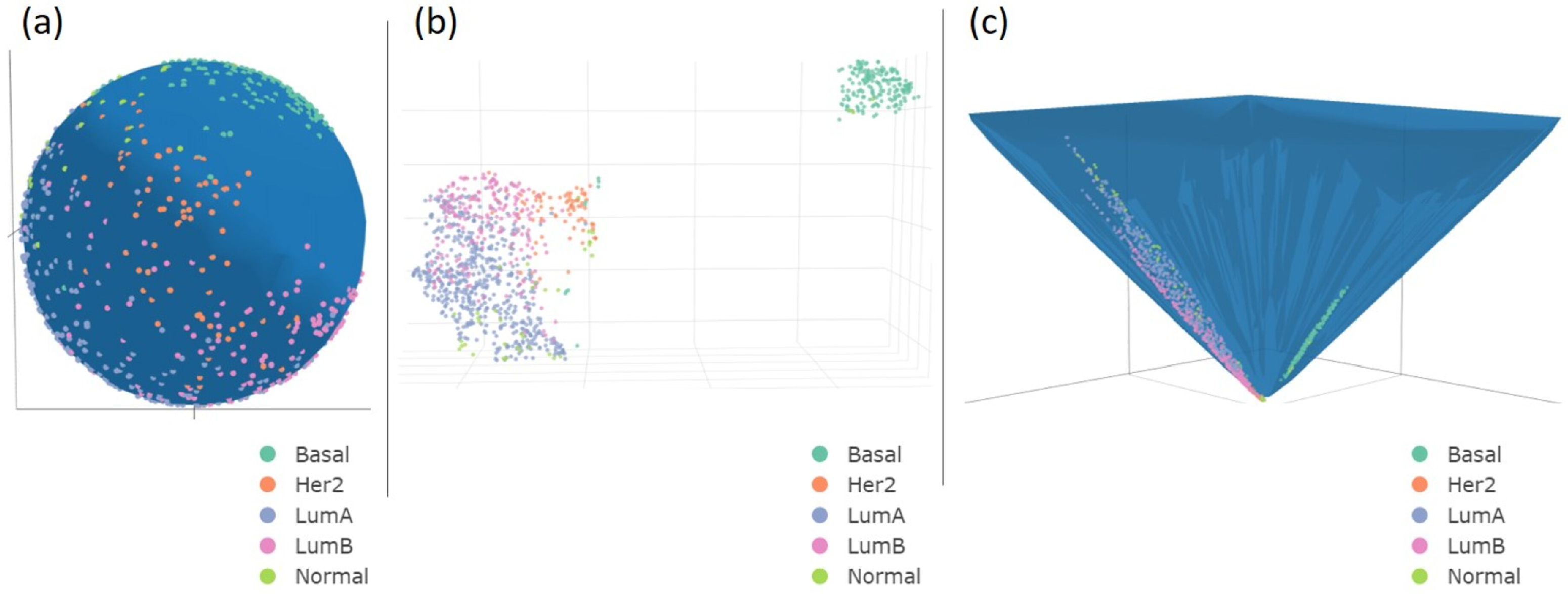
3.1. UMAP
3.2. Clustering
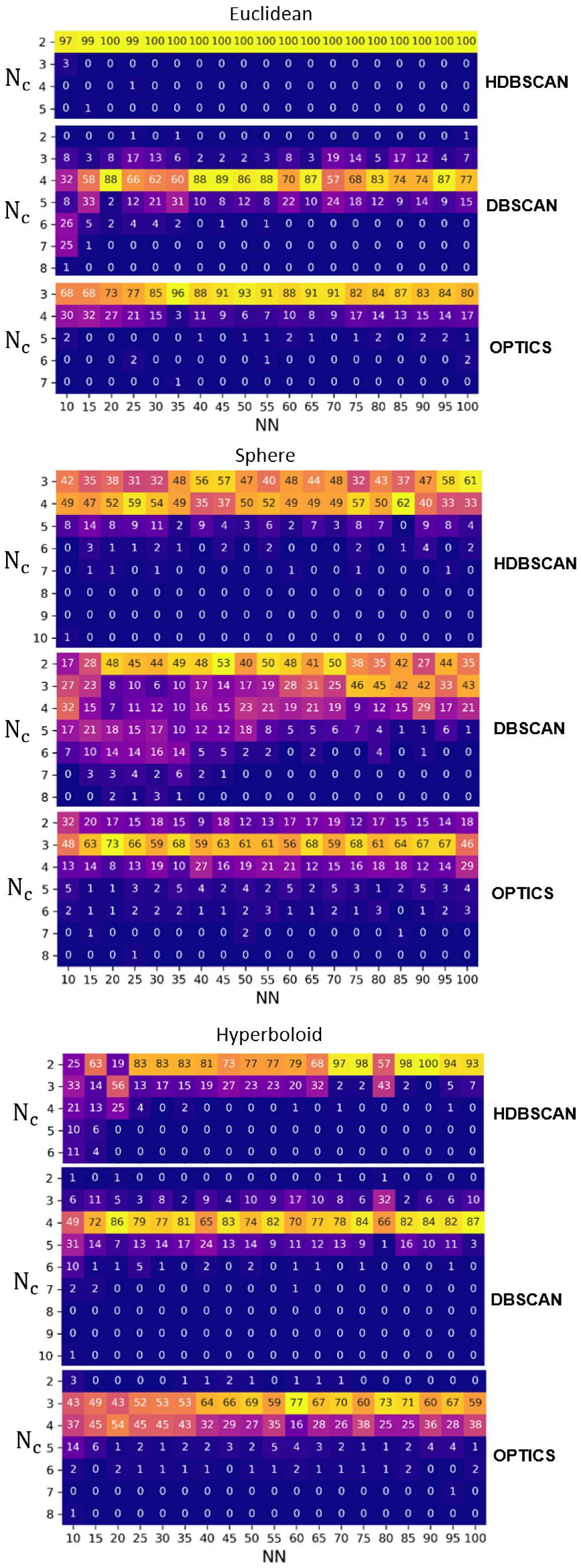
3.2.1. Irreproducibility Issues
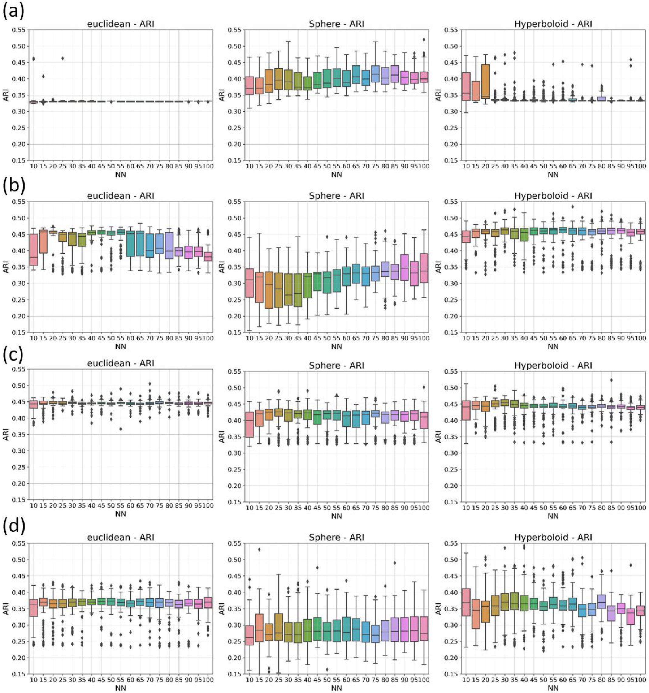
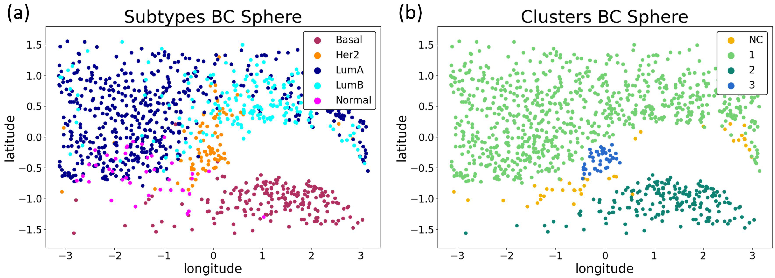
3.2.2. Reproducible Results
- N and ARI equal to 0.47 (spherical metric), N and ARI equal to 0.33 (Euclidean metric), and N and ARI equal to 0.46 (hyperbolic metric), for HDBSCAN;
- N and ARI equal to 0.39 (spherical metric), N and ARI equal to 0.45 (Euclidean metric), and N and ARI equal to 0.46 (hyperbolic metric), for DBSCAN;
- N and ARI equal to 0.28 (spherical metric), N and ARI equal to 0.38 (Euclidean metric), and N and ARI equal to 0.38 (hyperbolic metric), for agglomerative clustering;
- N and ARI equal to 0.41 (spherical metric), N and ARI equal to 0.44 (Euclidean metric), and N and ARI equal to 0.44 (hyperbolic metric), for OPTICS.
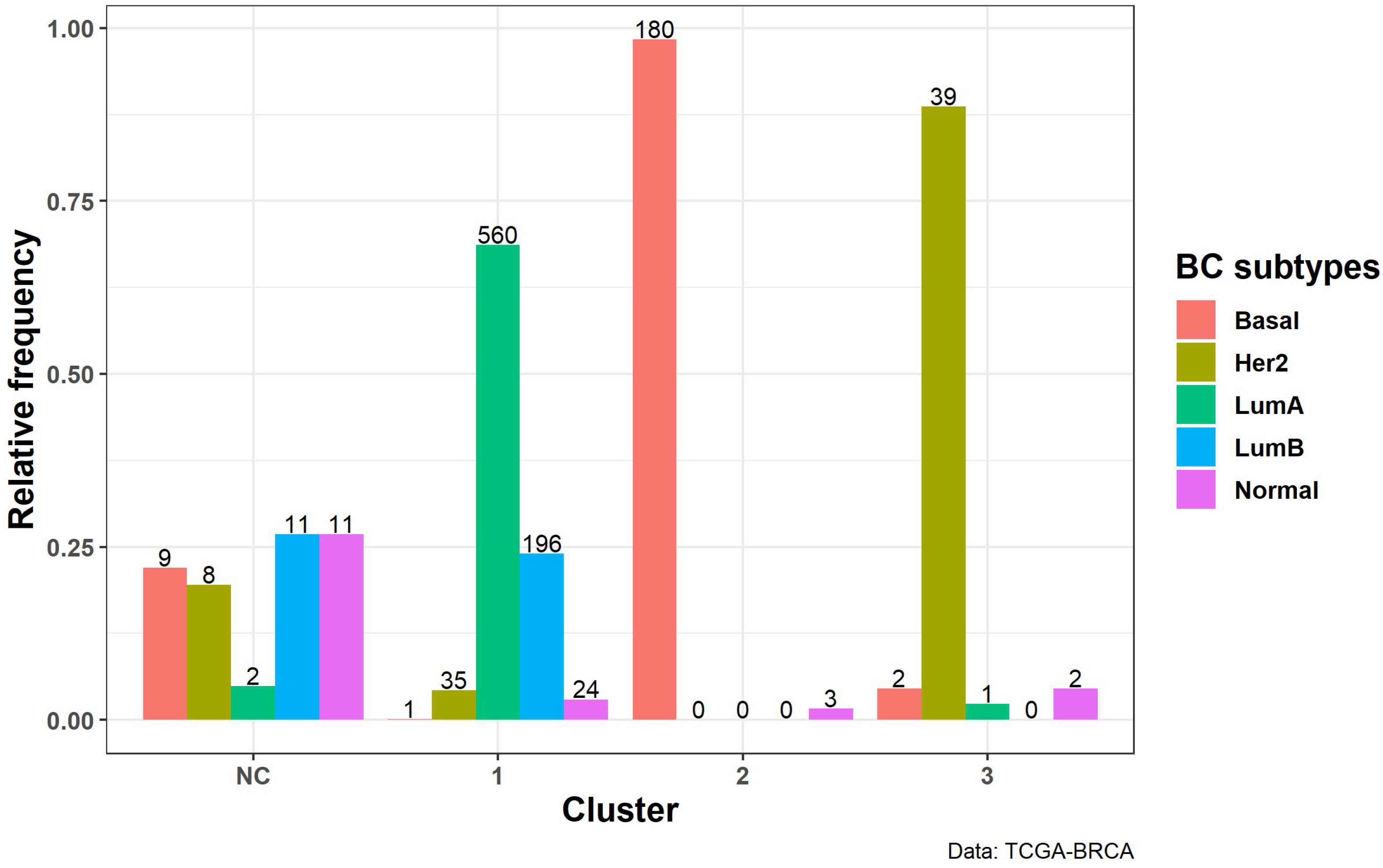
3.2.3. Biological Interpretation
4. Discussion
5. Conclusions
Author Contributions
Funding
Institutional Review Board Statement
Informed Consent Statement
Data Availability Statement
Acknowledgments
Conflicts of Interest
Appendix A
Appendix A.1. Reproducibility
- (1)
- comparison in terms of ARI of two clustering outputs generated by HDBSCAN applied to two separate runs of UMAP (NN ; spherical embedding);
- (2)
- for each , comparison in terms of ARI of two clustering outputs generated by two independent runs of our proposed pipeline.


| (A) | 1 Embedding Iter1 | (B) | 1 Embedding Iter2 | ||||||||
|---|---|---|---|---|---|---|---|---|---|---|---|
| Clusters | Clusters | ||||||||||
| NC | 1 | 2 | 3 | NC | 1 | 2 | 3 | ||||
| Basal | 1 | 1 | 184 | 6 | Basal | 8 | 0 | 179 | 5 | ||
| Her2 | 0 | 31 | 4 | 47 | Her2 | 5 | 41 | 0 | 36 | ||
| LumA | 1 | 553 | 8 | 1 | LumA | 9 | 339 | 0 | 215 | ||
| LumB | 2 | 200 | 1 | 4 | LumB | 9 | 132 | 0 | 66 | ||
| Normal | 1 | 24 | 12 | 3 | Normal | 12 | 21 | 3 | 4 | ||
| (C) | 100 Embeddings Iter1 | (D) | 100 Embeddings Iter2 | ||||||||
| Clusters | Clusters | ||||||||||
| NC | 1 | 2 | 3 | NC | 1 | 2 | 3 | ||||
| Basal | 9 | 1 | 180 | 2 | Basal | 9 | 1 | 180 | 2 | ||
| Her2 | 8 | 35 | 0 | 39 | Her2 | 7 | 35 | 0 | 40 | ||
| LumA | 2 | 560 | 0 | 1 | LumA | 3 | 559 | 0 | 1 | ||
| LumB | 11 | 196 | 0 | 0 | LumB | 9 | 198 | 0 | 0 | ||
| Normal | 11 | 24 | 3 | 2 | Normal | 10 | 24 | 3 | 3 | ||
Appendix A.2. Clustering Results
| HDBSCAN | Euclidean | Sphere | Hyperboloid | ||||||
|---|---|---|---|---|---|---|---|---|---|
| NN | Nclust | Ari | Homog | Nclust | Ari | Homog | Nclust | Ari | Homog |
| 10 | 2 | 0.33 | 0.31 | 4 | 0.45 | 0.43 | 3 | 0.46 | 0.42 |
| 15 | 2 | 0.33 | 0.32 | 4 | 0.46 | 0.44 | 2 | 0.33 | 0.32 |
| 20 | 2 | 0.33 | 0.32 | 4 | 0.46 | 0.44 | 3 | 0.45 | 0.42 |
| 25 | 2 | 0.33 | 0.32 | 4 | 0.46 | 0.44 | 2 | 0.33 | 0.32 |
| 30 | 2 | 0.33 | 0.32 | 4 | 0.46 | 0.44 | 2 | 0.33 | 0.32 |
| 35 | 2 | 0.33 | 0.32 | 4 | 0.45 | 0.43 | 2 | 0.33 | 0.32 |
| 40 | 2 | 0.33 | 0.32 | 3 | 0.37 | 0.35 | 2 | 0.33 | 0.32 |
| 45 | 2 | 0.33 | 0.32 | 3 | 0.37 | 0.35 | 2 | 0.33 | 0.32 |
| 50 | 2 | 0.33 | 0.32 | 4 | 0.46 | 0.43 | 2 | 0.33 | 0.32 |
| 55 | 2 | 0.33 | 0.32 | 4 | 0.46 | 0.43 | 2 | 0.33 | 0.32 |
| 60 | 2 | 0.33 | 0.32 | 4 | 0.46 | 0.43 | 2 | 0.33 | 0.32 |
| 65 | 2 | 0.33 | 0.32 | 4 | 0.47 | 0.43 | 2 | 0.33 | 0.32 |
| 70 | 2 | 0.33 | 0.32 | 4 | 0.47 | 0.43 | 2 | 0.33 | 0.32 |
| 75 | 2 | 0.33 | 0.32 | 4 | 0.47 | 0.43 | 2 | 0.33 | 0.32 |
| 80 | 2 | 0.33 | 0.32 | 4 | 0.46 | 0.43 | 2 | 0.33 | 0.32 |
| 85 | 2 | 0.33 | 0.32 | 4 | 0.46 | 0.43 | 2 | 0.33 | 0.32 |
| 90 | 2 | 0.33 | 0.32 | 3 | 0.45 | 0.4 | 2 | 0.33 | 0.32 |
| 95 | 2 | 0.33 | 0.32 | 3 | 0.45 | 0.39 | 2 | 0.33 | 0.32 |
| 100 | 2 | 0.33 | 0.32 | 3 | 0.46 | 0.4 | 2 | 0.33 | 0.32 |
| 10 | 4 | 0.39 | 0.42 | 4 | 0.28 | 0.39 | 4 | 0.45 | 0.43 |
| 15 | 4 | 0.45 | 0.42 | 2 | 0.33 | 0.32 | 4 | 0.46 | 0.43 |
| 20 | 4 | 0.45 | 0.43 | 2 | 0.33 | 0.32 | 4 | 0.45 | 0.42 |
| 25 | 4 | 0.45 | 0.43 | 2 | 0.33 | 0.32 | 4 | 0.46 | 0.43 |
| 30 | 4 | 0.45 | 0.43 | 2 | 0.32 | 0.31 | 4 | 0.45 | 0.43 |
| 35 | 4 | 0.45 | 0.42 | 2 | 0.31 | 0.3 | 4 | 0.45 | 0.43 |
| 40 | 4 | 0.45 | 0.42 | 2 | 0.32 | 0.3 | 4 | 0.45 | 0.43 |
| 45 | 4 | 0.45 | 0.42 | 2 | 0.32 | 0.3 | 4 | 0.45 | 0.43 |
| 50 | 4 | 0.44 | 0.42 | 2 | 0.32 | 0.31 | 4 | 0.45 | 0.43 |
| 55 | 4 | 0.43 | 0.4 | 2 | 0.29 | 0.28 | 4 | 0.45 | 0.43 |
| 60 | 4 | 0.45 | 0.42 | 2 | 0.31 | 0.29 | 4 | 0.45 | 0.43 |
| 65 | 4 | 0.45 | 0.42 | 2 | 0.32 | 0.31 | 4 | 0.45 | 0.43 |
| 70 | 4 | 0.36 | 0.38 | 2 | 0.32 | 0.3 | 4 | 0.45 | 0.43 |
| 75 | 4 | 0.39 | 0.38 | 3 | 0.37 | 0.38 | 4 | 0.45 | 0.43 |
| 80 | 4 | 0.37 | 0.36 | 3 | 0.38 | 0.38 | 4 | 0.45 | 0.43 |
| 85 | 4 | 0.37 | 0.36 | 2 | 0.32 | 0.31 | 4 | 0.44 | 0.43 |
| 90 | 4 | 0.38 | 0.37 | 3 | 0.4 | 0.39 | 4 | 0.45 | 0.43 |
| 95 | 4 | 0.37 | 0.36 | 2 | 0.32 | 0.31 | 4 | 0.45 | 0.43 |
| 100 | 4 | 0.36 | 0.36 | 3 | 0.39 | 0.38 | 4 | 0.44 | 0.42 |
| OPTICS | Euclidean | Sphere | Hyperboloid | ||||||
|---|---|---|---|---|---|---|---|---|---|
| NN | Nclust | Ari | Homog | Nclust | Ari | Homog | Nclust | Ari | Homog |
| 10 | 3 | 0.42 | 0.39 | 3 | 0.4 | 0.38 | 3 | 0.43 | 0.4 |
| 15 | 3 | 0.43 | 0.4 | 3 | 0.41 | 0.38 | 3 | 0.44 | 0.41 |
| 20 | 3 | 0.44 | 0.41 | 3 | 0.41 | 0.39 | 4 | 0.36 | 0.41 |
| 25 | 3 | 0.44 | 0.41 | 3 | 0.41 | 0.39 | 3 | 0.44 | 0.41 |
| 30 | 3 | 0.44 | 0.41 | 3 | 0.41 | 0.39 | 3 | 0.44 | 0.41 |
| 35 | 3 | 0.43 | 0.41 | 3 | 0.4 | 0.38 | 3 | 0.43 | 0.41 |
| 40 | 3 | 0.44 | 0.41 | 3 | 0.4 | 0.38 | 3 | 0.44 | 0.41 |
| 45 | 3 | 0.43 | 0.41 | 3 | 0.4 | 0.38 | 3 | 0.44 | 0.41 |
| 50 | 3 | 0.44 | 0.41 | 3 | 0.4 | 0.38 | 3 | 0.44 | 0.41 |
| 55 | 3 | 0.44 | 0.41 | 3 | 0.4 | 0.38 | 3 | 0.44 | 0.41 |
| 60 | 3 | 0.44 | 0.41 | 3 | 0.4 | 0.38 | 3 | 0.44 | 0.41 |
| 65 | 3 | 0.43 | 0.41 | 3 | 0.4 | 0.38 | 3 | 0.43 | 0.41 |
| 70 | 3 | 0.43 | 0.41 | 3 | 0.4 | 0.38 | 3 | 0.42 | 0.4 |
| 75 | 3 | 0.43 | 0.41 | 3 | 0.4 | 0.38 | 3 | 0.43 | 0.4 |
| 80 | 3 | 0.43 | 0.41 | 3 | 0.4 | 0.38 | 3 | 0.43 | 0.41 |
| 85 | 3 | 0.43 | 0.4 | 3 | 0.41 | 0.39 | 3 | 0.43 | 0.4 |
| 90 | 3 | 0.43 | 0.41 | 3 | 0.4 | 0.38 | 3 | 0.43 | 0.4 |
| 95 | 3 | 0.43 | 0.4 | 3 | 0.4 | 0.38 | 3 | 0.42 | 0.4 |
| 100 | 3 | 0.43 | 0.41 | 3 | 0.39 | 0.37 | 3 | 0.42 | 0.4 |
| 10 | 4 | 0.37 | 0.48 | 4 | 0.28 | 0.42 | 4 | 0.38 | 0.49 |
| 15 | 4 | 0.37 | 0.48 | 4 | 0.28 | 0.42 | 4 | 0.38 | 0.49 |
| 20 | 4 | 0.36 | 0.48 | 4 | 0.24 | 0.4 | 4 | 0.36 | 0.49 |
| 25 | 4 | 0.36 | 0.49 | 4 | 0.24 | 0.4 | 4 | 0.37 | 0.47 |
| 30 | 4 | 0.37 | 0.48 | 4 | 0.24 | 0.4 | 4 | 0.36 | 0.47 |
| 35 | 4 | 0.37 | 0.48 | 4 | 0.24 | 0.4 | 4 | 0.36 | 0.47 |
| 40 | 4 | 0.37 | 0.49 | 4 | 0.24 | 0.41 | 4 | 0.36 | 0.47 |
| 45 | 4 | 0.38 | 0.49 | 4 | 0.24 | 0.4 | 4 | 0.36 | 0.47 |
| 50 | 4 | 0.38 | 0.49 | 4 | 0.24 | 0.4 | 4 | 0.35 | 0.47 |
| 55 | 4 | 0.38 | 0.49 | 4 | 0.24 | 0.4 | 4 | 0.35 | 0.47 |
| 60 | 4 | 0.37 | 0.49 | 4 | 0.24 | 0.41 | 4 | 0.35 | 0.47 |
| 65 | 4 | 0.37 | 0.48 | 4 | 0.24 | 0.41 | 4 | 0.35 | 0.47 |
| 70 | 4 | 0.38 | 0.49 | 4 | 0.24 | 0.4 | 4 | 0.36 | 0.48 |
| 75 | 4 | 0.37 | 0.49 | 4 | 0.24 | 0.4 | 4 | 0.36 | 0.48 |
| 80 | 4 | 0.37 | 0.48 | 4 | 0.24 | 0.4 | 4 | 0.35 | 0.48 |
| 85 | 4 | 0.37 | 0.49 | 4 | 0.24 | 0.4 | 4 | 0.36 | 0.48 |
| 90 | 4 | 0.38 | 0.49 | 4 | 0.24 | 0.4 | 4 | 0.35 | 0.48 |
| 95 | 4 | 0.37 | 0.48 | 4 | 0.24 | 0.39 | 4 | 0.34 | 0.47 |
| 100 | 4 | 0.38 | 0.49 | 4 | 0.24 | 0.41 | 4 | 0.34 | 0.47 |
References
- Baptiste, M.; Moinuddeen, S.S.; Soliz, C.L.; Ehsan, H.; Kaneko, G. Making sense of genetic information: The promising evolution of clinical stratification and precision oncology using machine learning. Genes 2021, 12, 722. [Google Scholar] [CrossRef]
- Sung, H.; Ferlay, J.; Siegel, R.L.; Laversanne, M.; Soerjomataram, I.; Jemal, A.; Bray, F. Global cancer statistics 2020: Globocan estimates of incidence and mortality worldwide for 36 cancers in 185 countries. CA Cancer J. Clin. 2021, 71, 209–249. Available online: https://acsjournals.onlinelibrary.wiley.com/doi/pdf/10.3322/caac.21660 (accessed on 20 April 2022). [CrossRef] [PubMed]
- Oze, I.; Ito, H.; Kasugai, Y.; Yamaji, T.; Kijima, Y.; Ugai, T.; Kasuga, Y.; Ouellette, T.K.; Taniyama, Y.; Koyanagi, Y.N.; et al. A personal breast cancer risk stratification model using common variants and environmental risk factors in japanese females. Cancers 2021, 13, 3796. [Google Scholar] [CrossRef] [PubMed]
- Russnes, H.G.; Lingjærde, O.C.; Børresen-Dale, A.-L.; Caldas, C. Breast cancer molecular stratification: From intrinsic subtypes to integrative clusters. Am. J. Pathol. 2017, 187, 2152–2162. [Google Scholar] [CrossRef]
- Wordsworth, S.; Doble, B.; Payne, K.; Buchanan, J.; Marshall, D.A.; McCabe, C.; Regier, D.A. Using “big data” in the cost-effectiveness analysis of next-generation sequencing technologies: Challenges and potential solutions. Value Health 2018, 21, 1048–1053. [Google Scholar] [CrossRef] [Green Version]
- Arakelyan, A.; Melkonyan, A.; Hakobyan, S.; Boyarskih, U.; Simonyan, A.; Nersisyan, L.; Nikoghosyan, M.; Filipenko, M.; Binder, H. Transcriptome patterns of brca1-and brca2-mutated breast and ovarian cancers. Int. J. Mol. Sci. 2021, 22, 1266. [Google Scholar] [CrossRef] [PubMed]
- Wang, M.; Klevebring, D.; Lindberg, J.; Czene, K.; Grönberg, H.; Rantalainen, M. Determining breast cancer histological grade from rna-sequencing data. Breast Cancer Res. 2016, 18, 48. [Google Scholar] [CrossRef] [PubMed] [Green Version]
- Hao, Y.; He, L.; Zhou, Y.; Zhao, Y.; Li, M.; Jing, R.; Wen, Z. Improving model performance on the stratification of breast cancer patients by integrating multiscale genomic features. BioMed Res. Int. 2020, 2020, 1475368. [Google Scholar] [CrossRef]
- Altman, N.; Krzywinski, M. The curse(s) of dimensionality. Nat. Methods 2018, 15, 399–400. [Google Scholar] [CrossRef] [PubMed]
- Townes, F.W.; Hicks, S.C.; Aryee, M.J.; Irizarry, R.A. Feature selection and dimension reduction for single-cell rna-seq based on a multinomial model. Genome Biol. 2019, 20, 295. [Google Scholar] [CrossRef] [PubMed] [Green Version]
- Sun, X.; Liu, Y.; An, L. Ensemble dimensionality reduction and feature gene extraction for single-cell rna-seq data. Nat. Commun. 2020, 11, 5853. [Google Scholar] [CrossRef] [PubMed]
- McInnes, L.; Healy, J.; Melville, J. Umap: Uniform manifold approximation and projection for dimension reduction. arXiv 2018, arXiv:1802.03426. [Google Scholar]
- Yang, Y.; Sun, H.; Zhang, Y.; Zhang, T.; Gong, J.; Wei, Y.; Duan, Y.-G.; Shu, M.; Yang, Y.; Wu, D.; et al. Dimensionality reduction by umap reinforces sample heterogeneity analysis in bulk transcriptomic data. Cell Rep. 2021, 36, 109442. [Google Scholar] [CrossRef] [PubMed]
- Lebedev, T.; Vagapova, E.; Spirin, P.; Rubtsov, P.; Astashkova, O.; Mikheeva, A.; Sorokin, M.; Vladimirova, U.; Suntsova, M.; Konovalov, D.; et al. Growth factor signaling predicts therapy resistance mechanisms and defines neuroblastoma subtypes. Oncogene 2021, 40, 6258–6272. [Google Scholar] [CrossRef]
- Dorrity, M.W.; Saunders, L.M.; Queitsch, C.; Fields, S.; Trapnell, C. Dimensionality reduction by umap to visualize physical and genetic interactions. Nat. Commun. 2020, 11, 1537. [Google Scholar] [CrossRef] [PubMed] [Green Version]
- Cao, J.; Spielmann, M.; Qiu, X.; Huang, X.; Ibrahim, D.M.; Hill, A.J.; Zhang, F.; Mundlos, S.; Christiansen, L.; Steemers, F.J. The single-cell transcriptional landscape of mammalian organogenesis. Nature 2019, 566, 496–502. [Google Scholar] [CrossRef] [PubMed]
- Maćkiewicz, A.; Ratajczak, W. Principal components analysis (pca). Comput. Geosci. 1993, 19, 303–342. [Google Scholar] [CrossRef]
- Leelatian, N.; Sinnaeve, J.; Mistry, A.M.; Barone, S.M.; Brockman, A.A.; Diggins, K.E.; Greenplate, A.R.; Weaver, K.D.; Thompson, R.C.; Chambless, L.B. Unsupervised machine learning reveals risk stratifying glioblastoma tumor cells. eLife 2020, 9, e56879. [Google Scholar] [CrossRef]
- Becht, E.; McInnes, L.; Healy, J.; Dutertre, C.-A.; Kwok, I.W.; Ng, L.G.; Ginhoux, F.; Newell, E.W. Dimensionality reduction for visualizing single-cell data using umap. Nat. Biotechnol. 2019, 37, 38–44. [Google Scholar] [CrossRef] [PubMed]
- Allaoui, M.; Kherfi, M.L.; Cheriet, A. Considerably improving clustering algorithms using umap dimensionality reduction technique: A comparative study. In International Conference on Image and Signal Processing; Springer: Berlin/Heidelberg, Germany, 2020; pp. 317–325. [Google Scholar]
- Gu, A.; Sala, F.; Gunel, B.; Ré, C. Learning mixed-curvature representations in product spaces. In Proceedings of the International Conference on Learning Representations, Vancouver, BC, Canada, 30 April–3 May 2018. [Google Scholar]
- Ding, J.; Regev, A. Deep generative model embedding of single-cell RNA-Seq profiles on hyperspheres and hyperbolic spaces. Nat. Commun. 2019, 12, 1–17. [Google Scholar] [CrossRef] [PubMed]
- Nickel, M.; Kiela, D. Learning continuous hierarchies in the lorentz model of hyperbolic geometry. In Proceedings of the International Conference on Machine Learning, Stockholm, Sweden, 10–15 July 2018; pp. 3779–3788. [Google Scholar]
- He, Z.; Zhang, J.; Yuan, X.; Xi, J.; Liu, Z.; Zhang, Y. Stratification of breast cancer by integrating gene expression data and clinical variables. Molecules 2019, 24, 631. [Google Scholar] [CrossRef] [PubMed] [Green Version]
- Liu, J.; Lichtenberg, T.; Hoadley, K.A.; Poisson, L.M.; Lazar, A.J.; Cherniack, A.D.; Kovatich, A.J.; Benz, C.C.; Levine, D.A.; Lee, A.V. An integrated tcga pan-cancer clinical data resource to drive high-quality survival outcome analytics. Cell 2018, 173, 400–416. [Google Scholar] [CrossRef] [Green Version]
- Ali, M.; Jones, M.W.; Xie, X.; Williams, M. Timecluster: Dimension reduction applied to temporal data for visual analytics. Vis. Comput. 2019, 35, 1013–1026. [Google Scholar] [CrossRef] [Green Version]
- Pealat, C.; Bouleux, G.; Cheutet, V. Improved time-series clustering with umap dimension reduction method. In Proceedings of the 2020 25th International Conference on Pattern Recognition (ICPR), Milan, Italy, 10–15 January 2021; pp. 5658–5665. [Google Scholar]
- Rand, W.M. Objective criteria for the evaluation of clustering methods. J. Am. Stat. Assoc. 1971, 66, 846–850. [Google Scholar] [CrossRef]
- Rosenberg, A.; Hirschberg, J. V-measure: A conditional entropy-based external cluster evaluation measure. In Proceedings of the 2007 Joint Conference on Empirical Methods in Natural Language Processing and Computational Natural Language Learning (EMNLP-CoNLL), Prague, Czech Republic, 28–30 June 2007; pp. 410–420. [Google Scholar]
- Diaz-Papkovich, A.; Anderson-Trocmé, L.; Gravel, S. A review of umap in population genetics. J. Hum. Genet. 2021, 66, 85–91. [Google Scholar] [CrossRef] [PubMed]
- Aalto, M.; Verma, N. Metric learning on manifolds. arXiv 2019, arXiv:1902.01738. [Google Scholar]
- Campello, R.J.; Moulavi, D.; Sander, J. Density-based clustering based on hierarchical density estimates. In Pacific-Asia Conference on Knowledge Discovery and Data Mining; Springer: Berlin/Heidelberg, Germany, 2013; pp. 160–172. [Google Scholar]
- Ester, M.; Kriegel, H.-P.; Kuntze, D.; Sander, J.; Xu, X. A density-based algorithm for discovering clusters in large spatial databases with noise. In Proceedings of the Second International Conference on Knowledge Discovery and Data Mining, Portland, OR, USA, 2–4 August 1996; Volume 96, pp. 226–231. [Google Scholar]
- Ankerst, M.; Breunig, M.M.; Kriegel, H.P.; Sander, J. OPTICS: Ordering points to identify the clustering structure. ACM Sigmod Rec. 1999, 28, 49–60. [Google Scholar] [CrossRef]
- Day, W.H.; Edelsbrunner, H. Efficient algorithms for agglomerative hierarchical clustering methods. J. Classif. 1984, 1, 7–24. [Google Scholar] [CrossRef]
- Jamail, I.; Moussa, A. Current state-of-the-art of clustering methods for gene expression data with rna-seq. In Pattern Recognition; IntechOpen: London, UK, 2020. [Google Scholar]
- Santos, J.M.; Embrechts, M. On the use of the adjusted rand index as a metric for evaluating supervised classification. In Proceedings of the International Conference on Artificial Neural Networks, Limassol, Cyprus, 14–17 September 2009; Springer: Berlin/Heidelberg, Germany, 2009; pp. 175–184. [Google Scholar]
- Higham, D.J.; Kalna, G.; Kibble, M. Spectral clustering and its use in bioinformatics. J. Comput. Appl. Math. 2007, 204, 25–37. [Google Scholar] [CrossRef] [Green Version]
- Gaynor, S.M.; Lin, X.; Quackenbush, J. Spectral clustering in regression-based biological networks. bioRxiv 2019, 651950. [Google Scholar] [CrossRef]
- Huang, G.T.; Cunningham, K.I.; Benos, P.V.; Chennubhotla, C.S. Spectral clustering strategies for heterogeneous disease expression data. In Biocomputing 2013; World Scientific: Singapore, 2013; pp. 212–223. [Google Scholar]
- Larsen, M.J.; Kruse, T.A.; Tan, Q.; Laenkholm, A.-V.; Bak, M.; Lykkesfeldt, A.E.; Sørensen, K.P.; Hansen, T.v.O.; Ejlertsen, B.; Gerdes, A.-M. Classifications within molecular subtypes enables identification of brca1/brca2 mutation carriers by rna tumor profiling. PLoS ONE 2013, 8, e64268. [Google Scholar] [CrossRef] [PubMed] [Green Version]
- Bao, X.; Shi, R.; Zhao, T.; Wang, Y.; Anastasov, N.; Rosemann, M.; Fang, W. Integrated analysis of single-cell rna-seq and bulk rna-seq unravels tumour heterogeneity plus m2-like tumour-associated macrophage infiltration and aggressiveness in tnbc. Cancer Immunol. Immunother. 2021, 70, 189–202. [Google Scholar] [CrossRef]
- Landry, A.P.; Balas, M.; Alli, S.; Spears, J.; Zador, Z. Distinct regional ontogeny and activation of tumor associated macrophages in human glioblastoma. Sci. Rep. 2020, 10, 19542. [Google Scholar] [CrossRef] [PubMed]
- Chari, T.; Banerjee, J.; Pachter, L. The specious art of single-cell genomics. bioRxiv 2021. [Google Scholar] [CrossRef]
- Ektefaie, Y.; Yuan, W.; Dillon, D.A.; Lin, N.U.; Golden, J.A.; Kohane, I.S.; Yu, K.H. Integrative multiomics-histopathology analysis for breast cancer classification. NPJ Breast Cancer 2021, 7, 147. [Google Scholar] [CrossRef] [PubMed]


Publisher’s Note: MDPI stays neutral with regard to jurisdictional claims in published maps and institutional affiliations. |
© 2022 by the authors. Licensee MDPI, Basel, Switzerland. This article is an open access article distributed under the terms and conditions of the Creative Commons Attribution (CC BY) license (https://creativecommons.org/licenses/by/4.0/).
Share and Cite
Bollon, J.; Assale, M.; Cina, A.; Marangoni, S.; Calabrese, M.; Salvemini, C.B.; Christille, J.M.; Gustincich, S.; Cavalli, A. Investigating How Reproducibility and Geometrical Representation in UMAP Dimensionality Reduction Impact the Stratification of Breast Cancer Tumors. Appl. Sci. 2022, 12, 4247. https://doi.org/10.3390/app12094247
Bollon J, Assale M, Cina A, Marangoni S, Calabrese M, Salvemini CB, Christille JM, Gustincich S, Cavalli A. Investigating How Reproducibility and Geometrical Representation in UMAP Dimensionality Reduction Impact the Stratification of Breast Cancer Tumors. Applied Sciences. 2022; 12(9):4247. https://doi.org/10.3390/app12094247
Chicago/Turabian StyleBollon, Jordy, Michela Assale, Andrea Cina, Stefano Marangoni, Matteo Calabrese, Chiara Beatrice Salvemini, Jean Marc Christille, Stefano Gustincich, and Andrea Cavalli. 2022. "Investigating How Reproducibility and Geometrical Representation in UMAP Dimensionality Reduction Impact the Stratification of Breast Cancer Tumors" Applied Sciences 12, no. 9: 4247. https://doi.org/10.3390/app12094247