
Continuous Rotor Dynamics of Multi-Disc and Multi-Span Rotor: A Theoretical and Numerical Investigation on the Identification of Bearing Coefficients from Unbalance Responses

Abstract
:1. Introduction
1.1. Background and Formulation of the Problem
1.2. Literature Survey
1.3. Scope and Contribution of This Study
1.4. Organization of the Paper
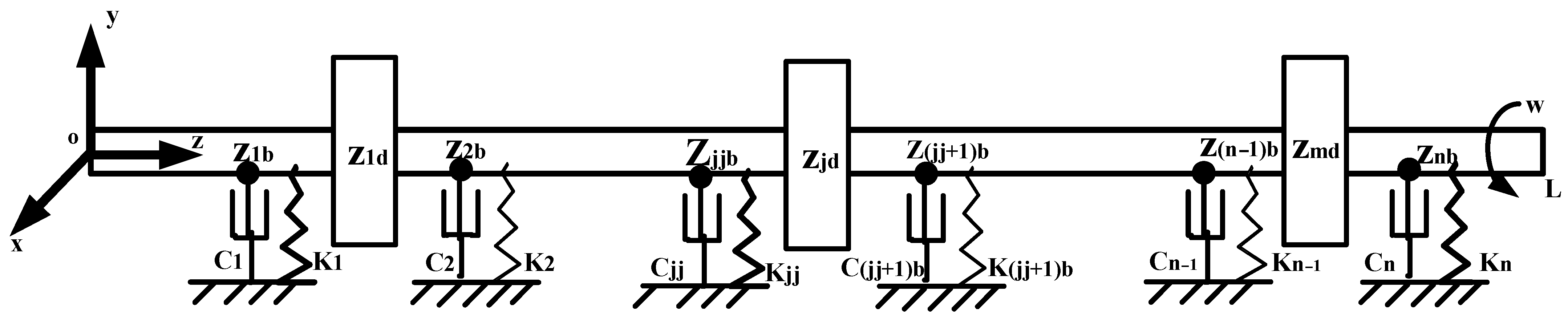
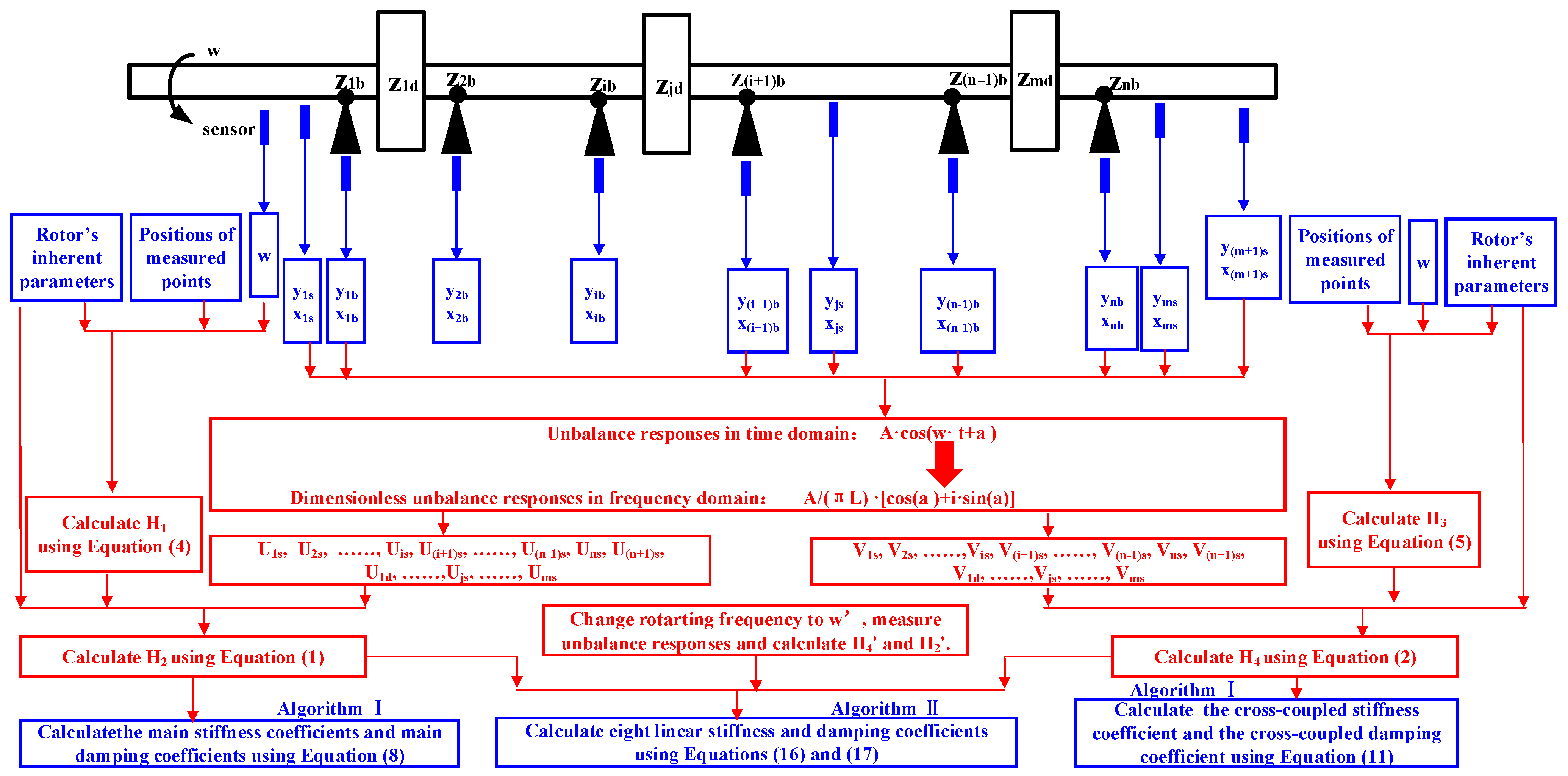
2. Theory
2.1. Algorithm I for Identification of Main Stiffness and Damping Coefficients of Rolling Bearings
2.2. Algorithm II for Identification of Bearings’ Main and Cross-Coupled Coefficients
2.3. Identification Procedures of the Two Algorithms
3. Numerical Simulations and Discussion
3.1. Methodology of Numerical Simulations
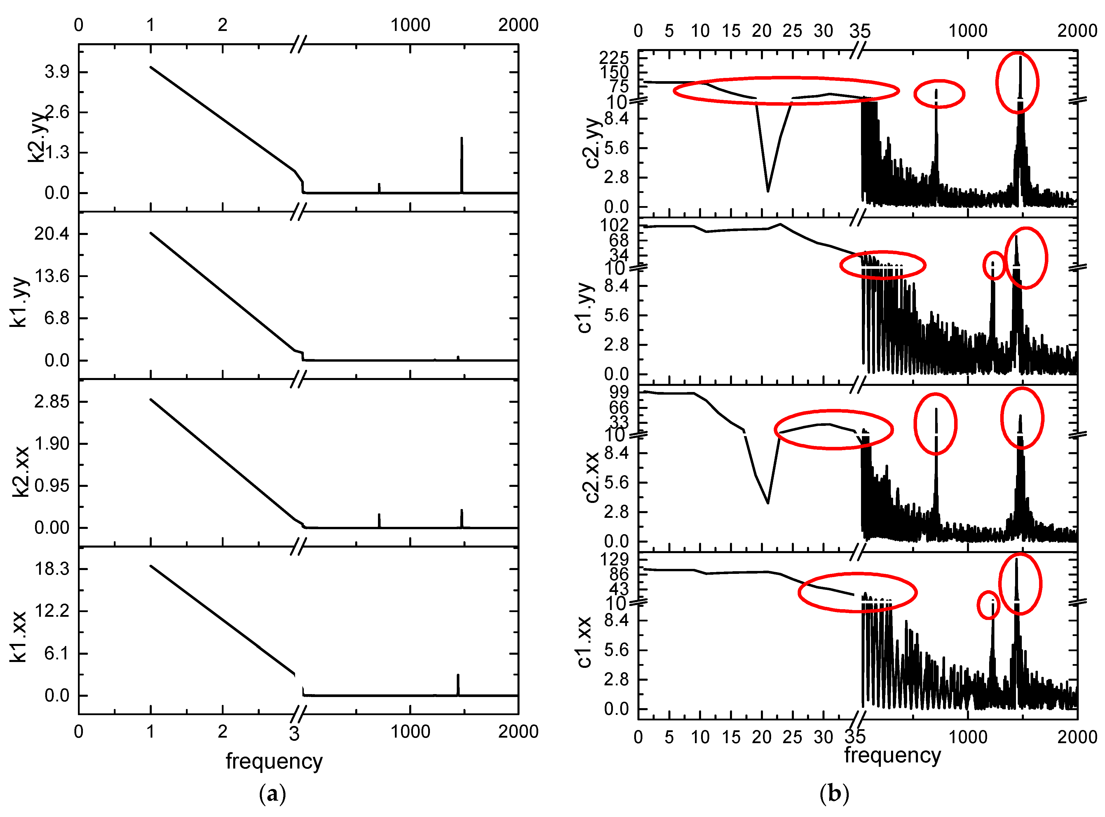
3.2. Finding of Adjustment Point
3.2.1. Results
The First Kind of Simulation Based on Algorithm I
- (1)
- #14 point as the last measuring point.
- (2)
- #29 point as the last measuring point.
- (3)
- #33 point as the last measuring point.
- (4)
- #49 point as the last measuring point.
- (5)
- #53 point as the last measuring point.
- (6)
- #69 point as the last measuring point.
- (7)
- #73 point as the last measuring point.
- (8)
- #91 point as the last measuring point.
The First Kind of Simulation Based on Algorithm II
- (1)
- Results of the computational example g4.4.
- (2)
- Results of the Computational Example h4.4.
3.2.2. Discussion
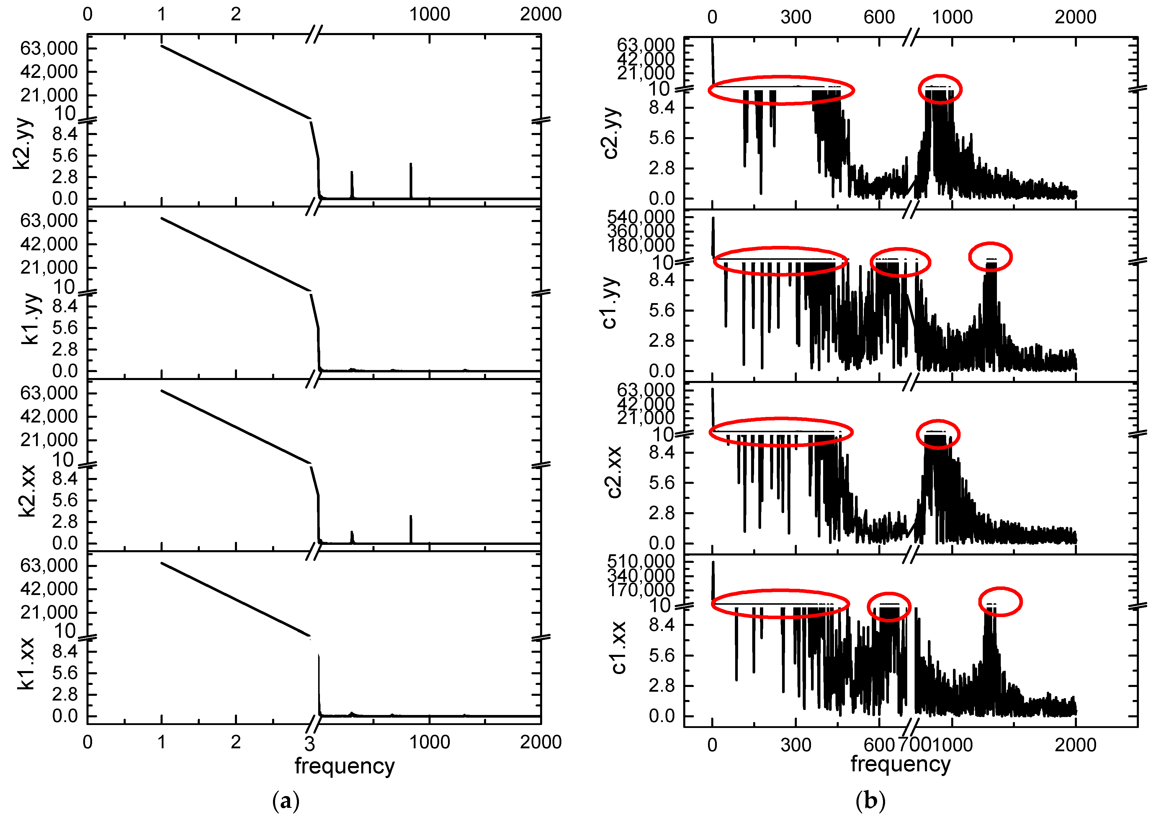
3.3. Application of Adjustment Point
3.3.1. Results
Results of the First Kind of Simulation
- (1)
- Simulation results based on Algorithm I.
- (2)
- Simulation results based on Algorithm II.
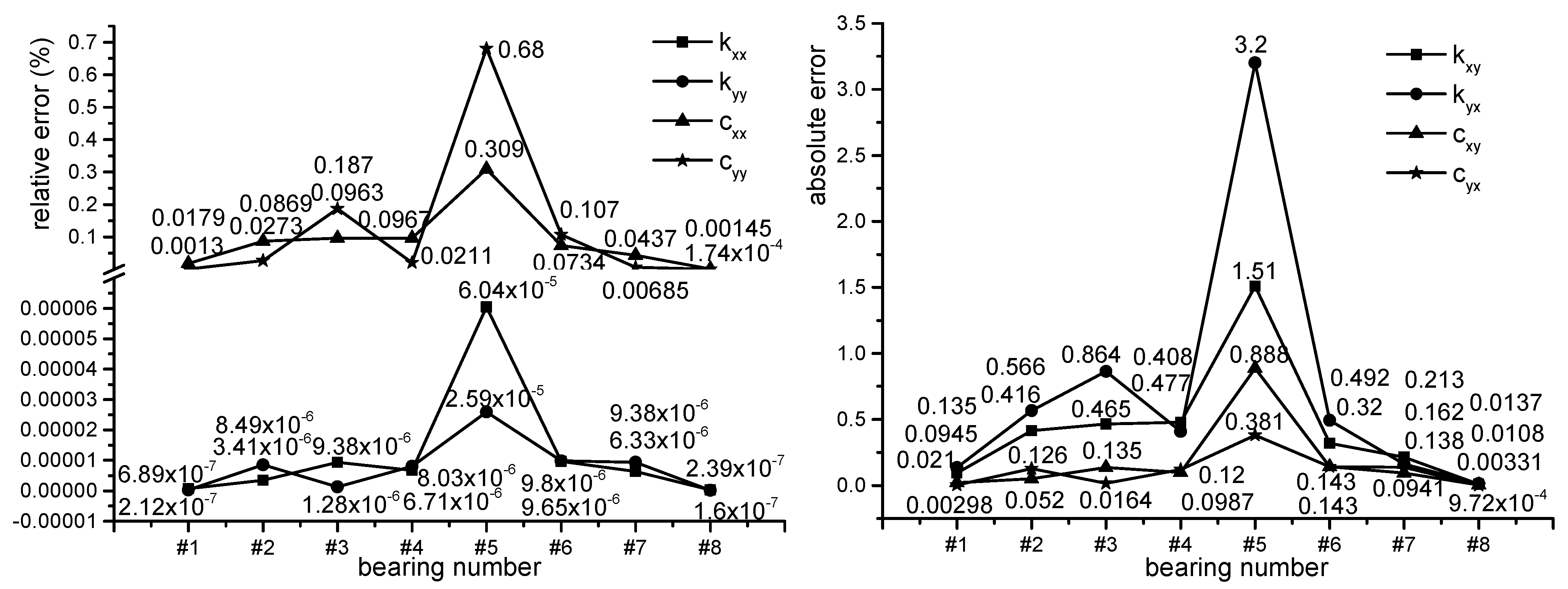
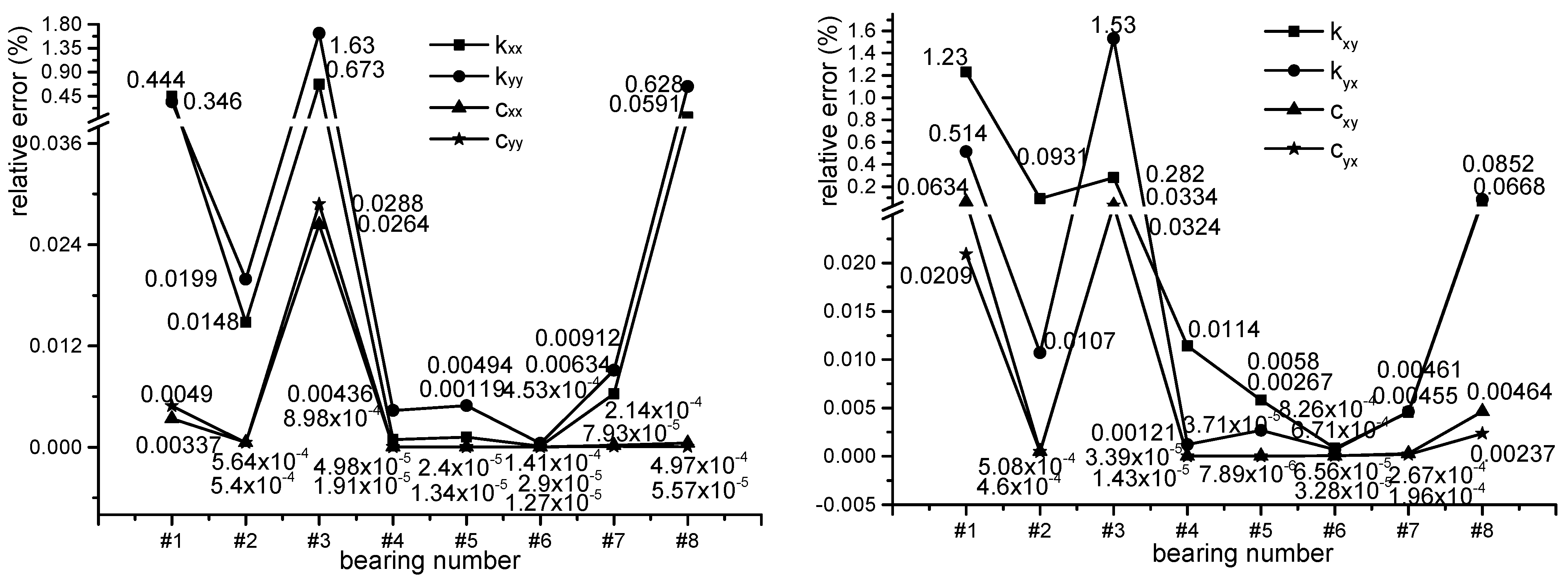
Results of the Second Kind of Simulation
- (1)
- Simulation results based on Algorithm I.
- (2)
- Simulation results based on Algorithm II.
3.3.2. Discussion
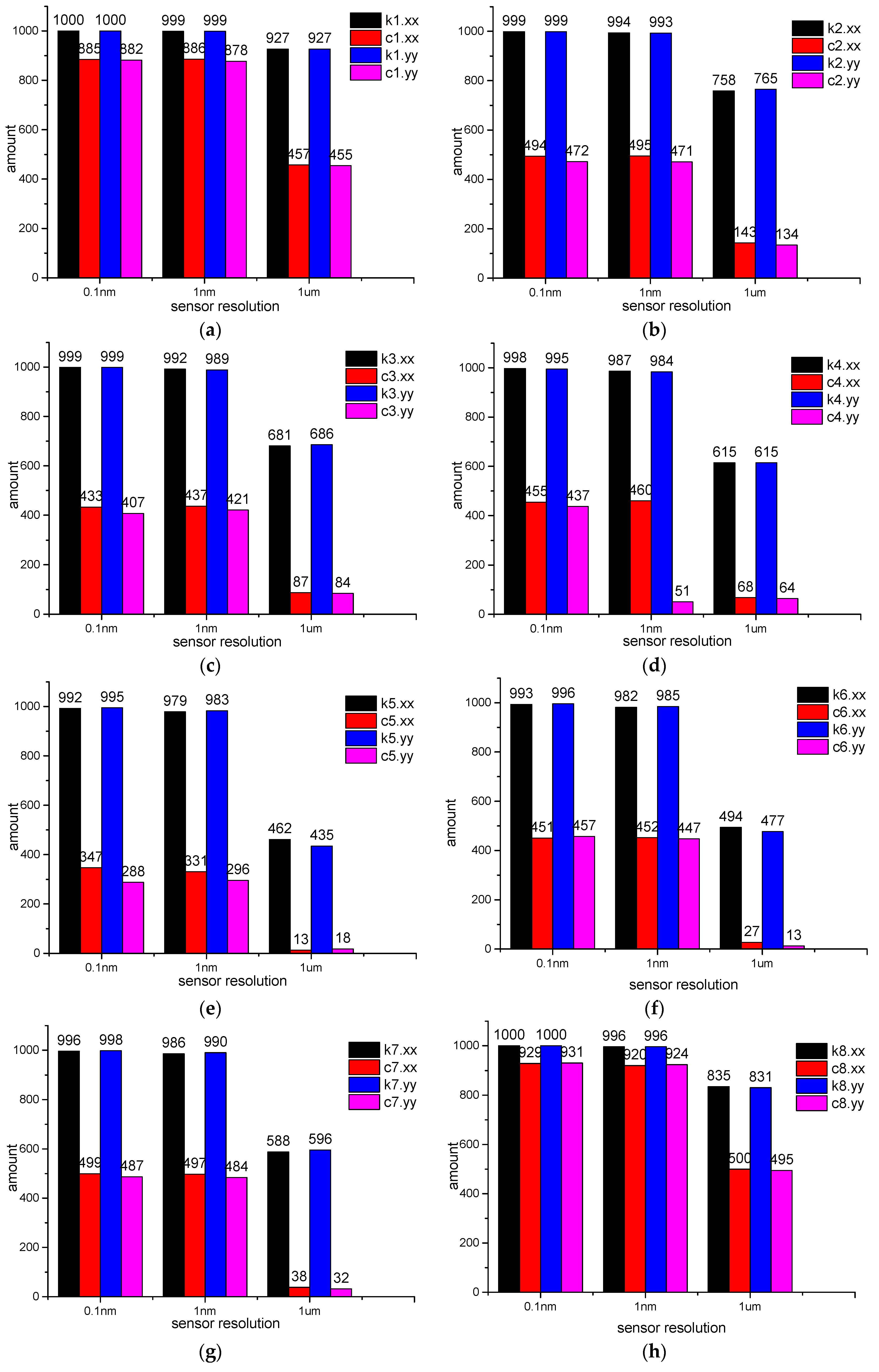
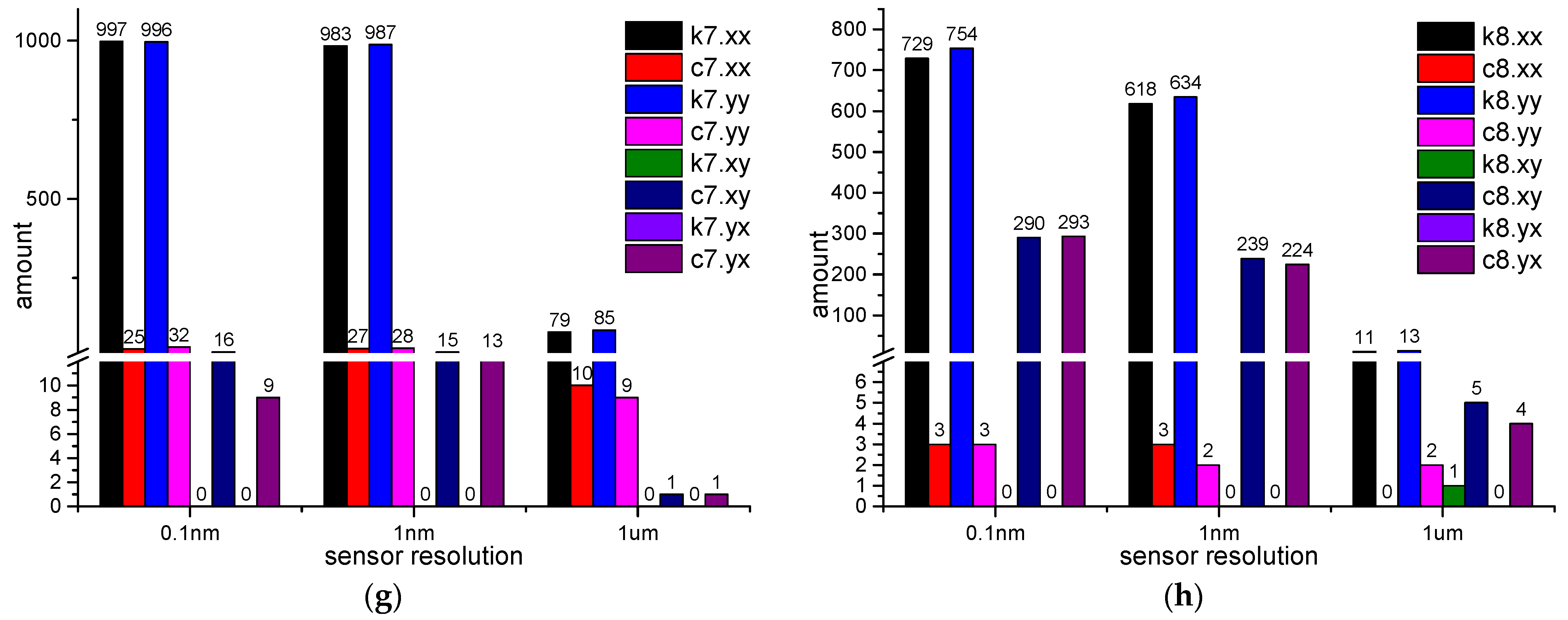
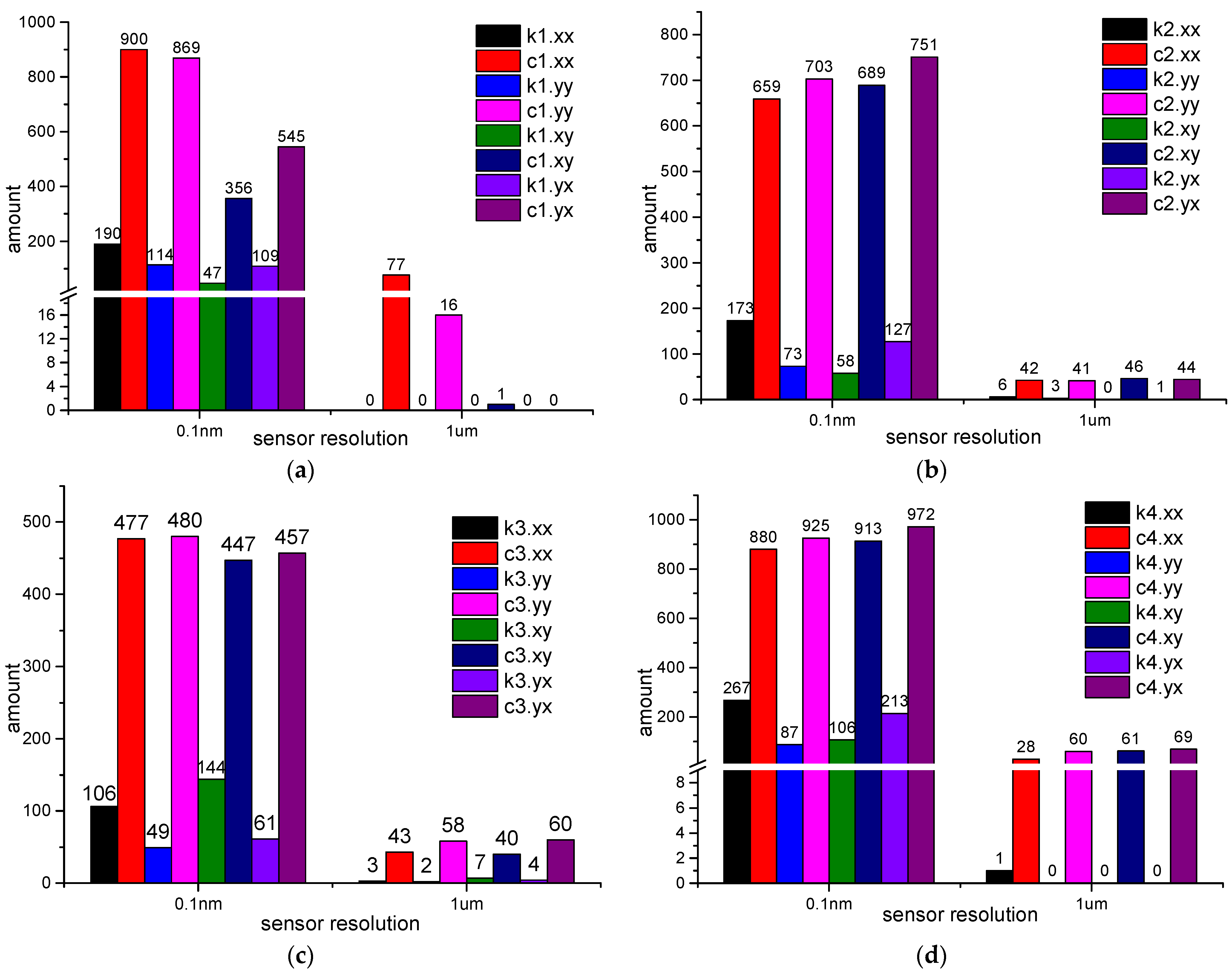
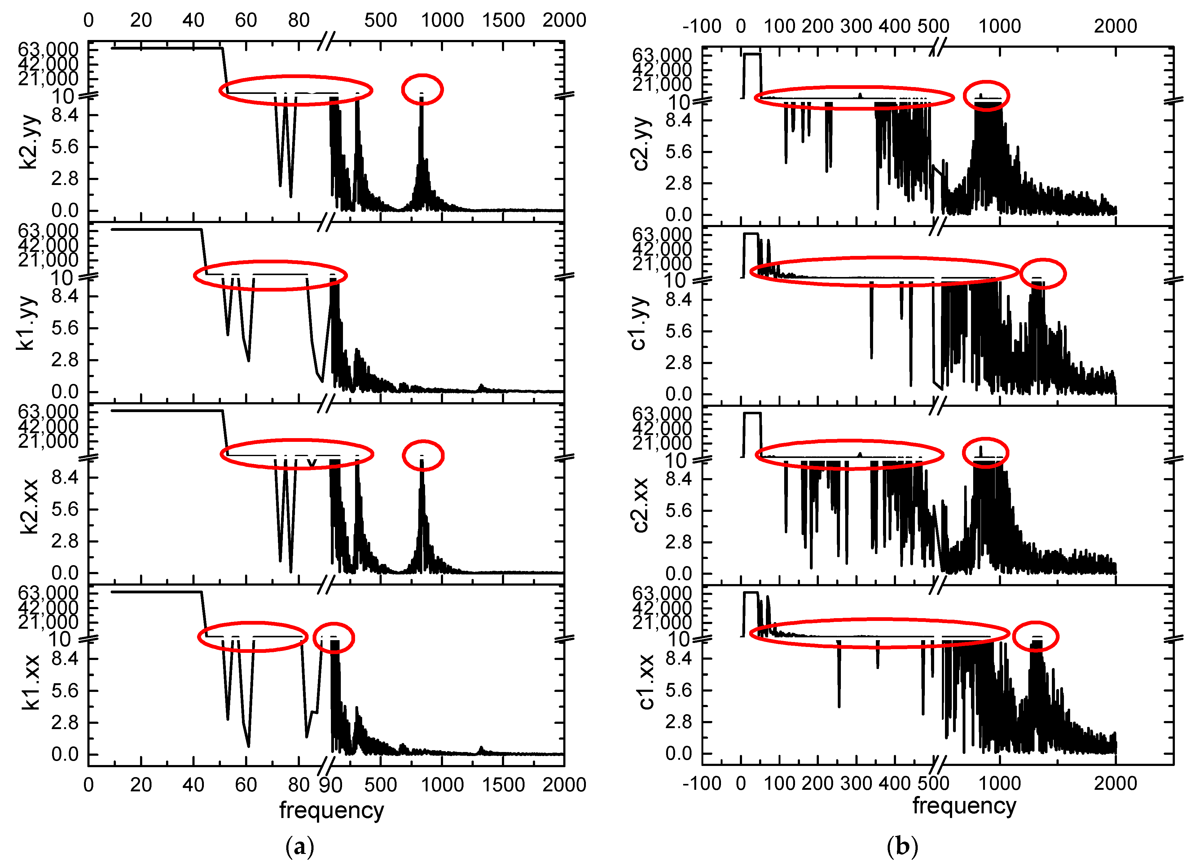
3.4. Effect of Sensor Resolution
3.4.1. Results
Simulations Results Based on Algorithm I
- (1)
- 0.1 nm resolution.
- (2)
- 1 nm resolution.
- (3)
- 1 um resolution.
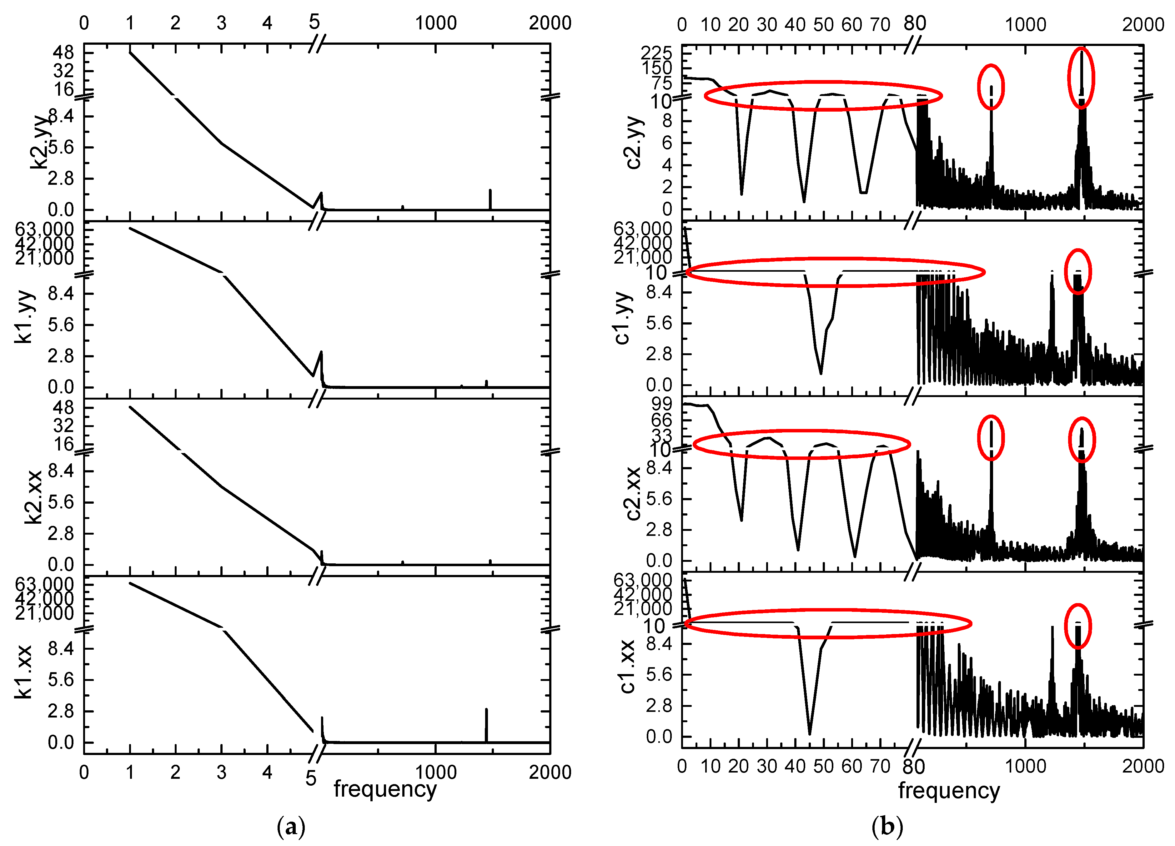
- (1)
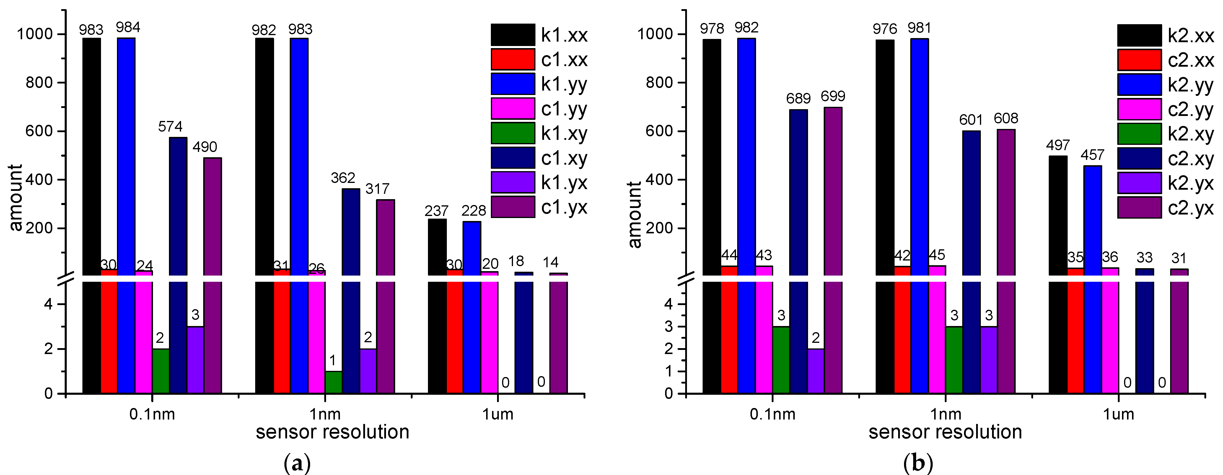
- The maximum relative error of the identified coefficient is very big and it appears at low frequency.
- (2)
- The main stiffness coefficients cannot be identified at 1 Hz when 1 nm resolution is used and the main stiffness coefficients cannot be identified from 1 to 33 Hz when 1 um resolution is applied.
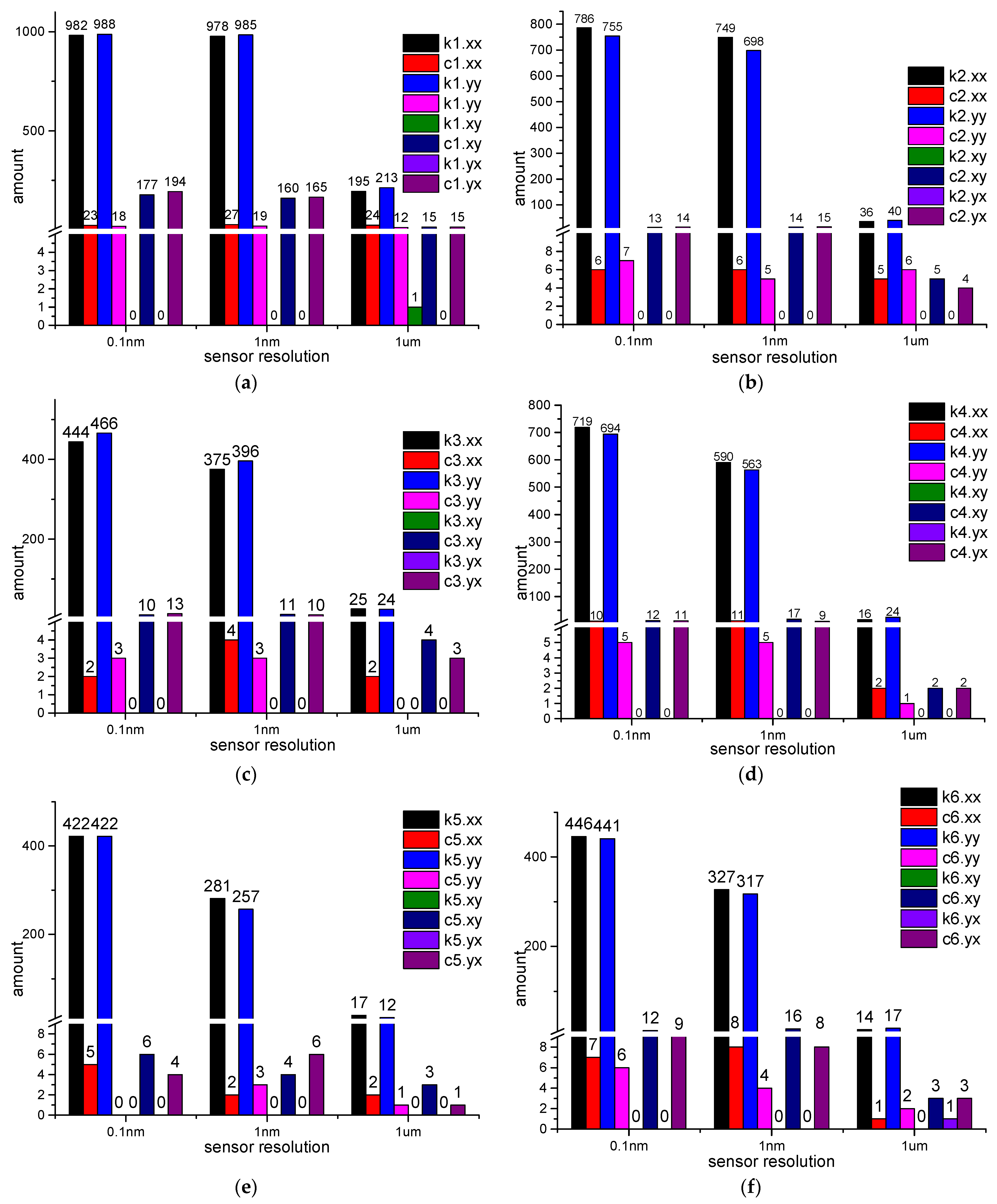
Simulations Results Based on Algorithm II
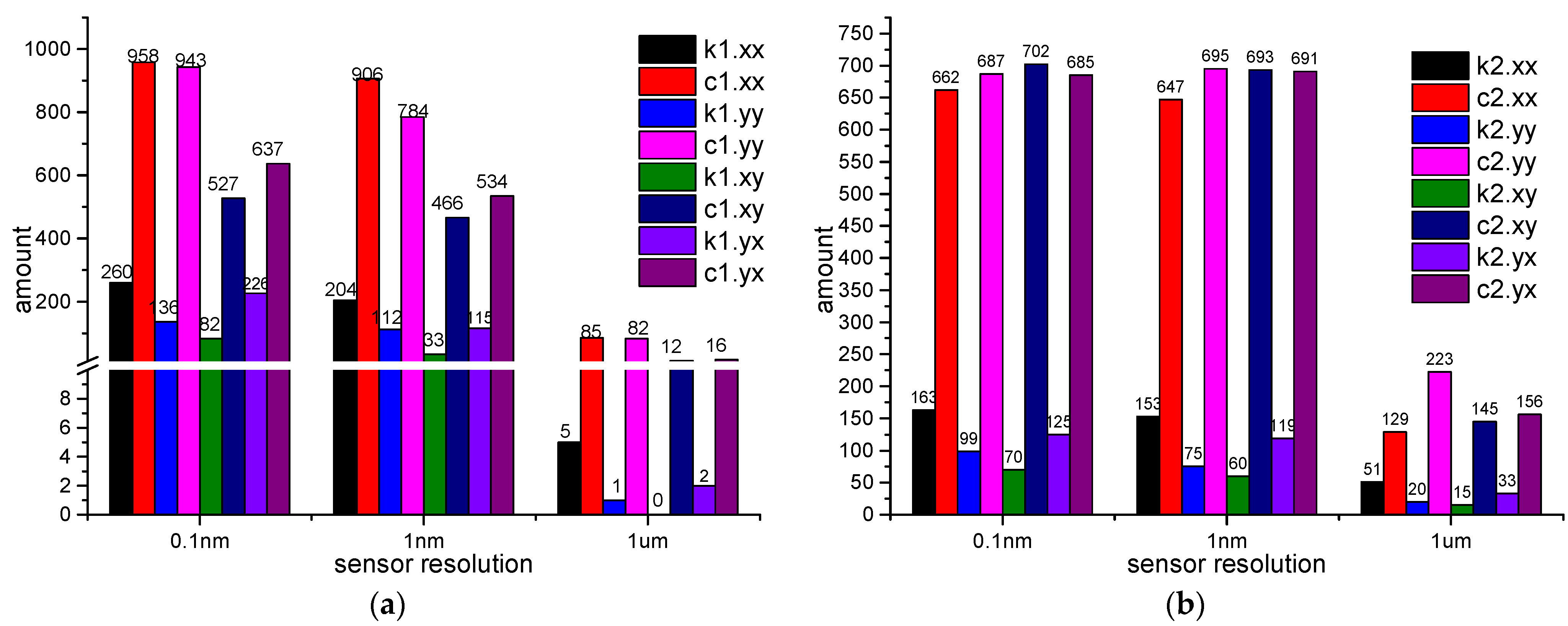
- (1)
- 0.1 nm resolution.
- (2)
- 1 nm resolution.
- (3)
- 1 um resolution.
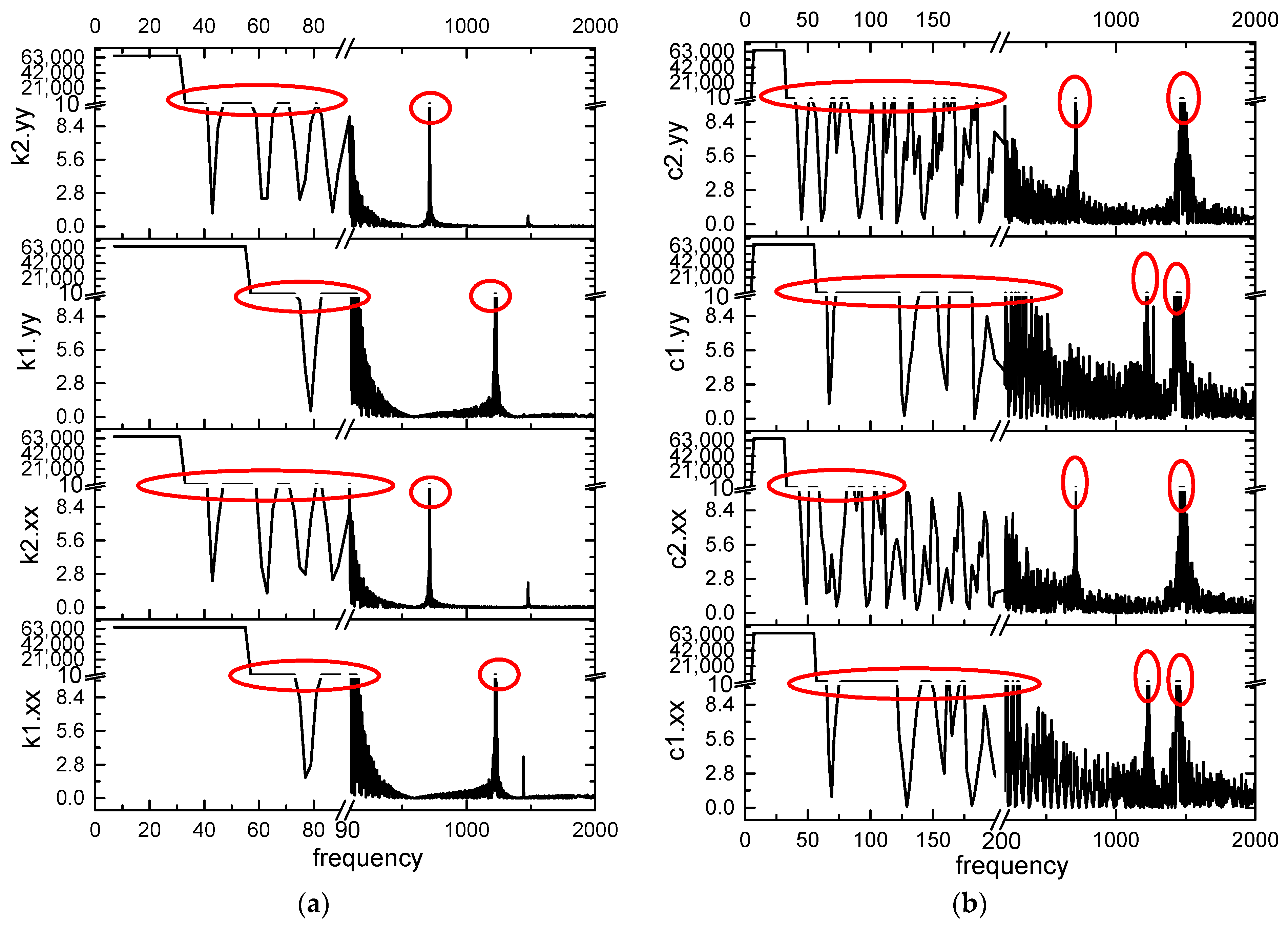
- (1)
- When the resolution is 1 nm, the coefficients of #1–3 bearing cannot be identified at 1 Hz. From 1 to 3 Hz, the coefficients of #4 and #6–8 bearing cannot be identified. From 1 to 5 Hz, the coefficients of #5 bearing cannot be identified.
- (2)
- When the resolution is 1 um, the coefficients of #1 bearing cannot be identified from 1 to 65 Hz. From 1 to 57 Hz, the coefficients of #2 bearing cannot be identified. From 1 to 83 Hz, the coefficients of #3 bearing cannot be identified. From 1 to 99 Hz, the coefficients of #4 bearing cannot be identified. From 1 to 163 Hz, the coefficients of #5 bearing cannot be identified. From 1 to 133 Hz, the coefficients of #6 bearing cannot be identified. From 1 to 97 Hz, the coefficients of #7 bearing cannot be identified. From 1 to 107 Hz, the coefficients of #8 bearing cannot be identified.
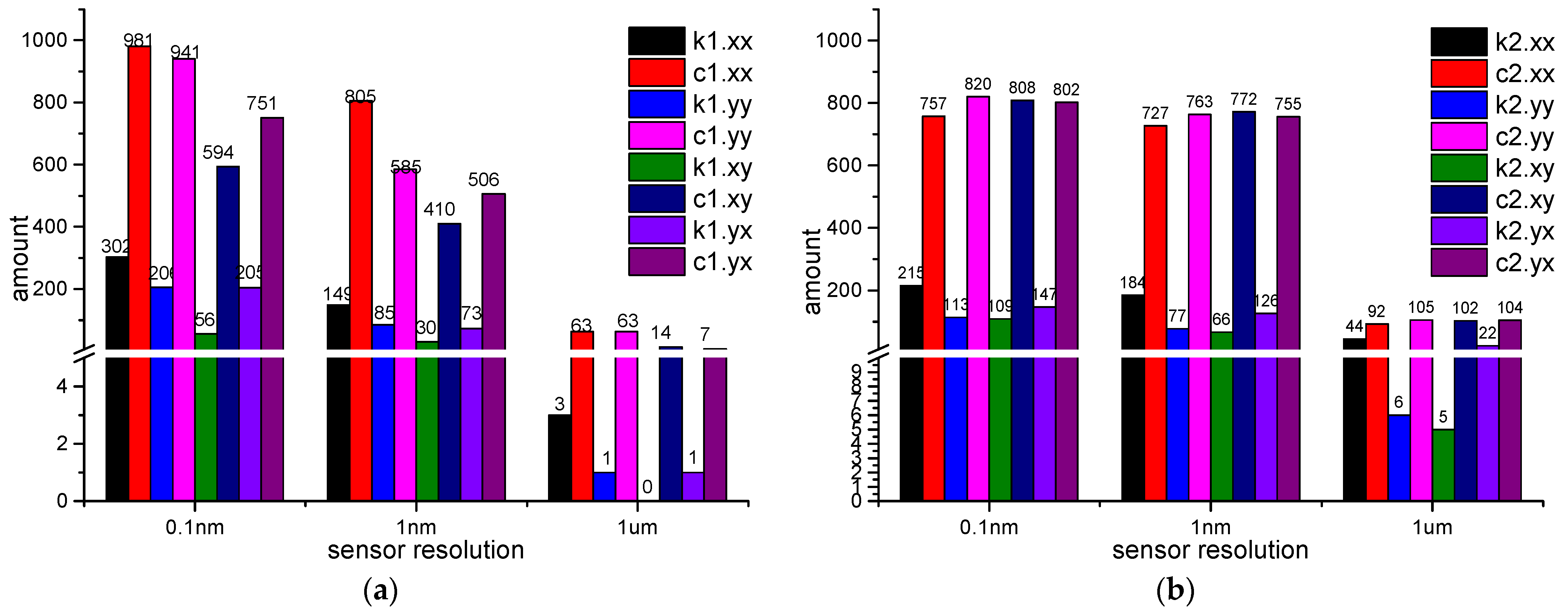
- (1)
- 0.1 nm resolution.
- (2)
- 1 um resolution.
- (1)
- At 1 Hz, k5.xx, k6.xx and k8.xx, c5.xx, c6.xx and c8.xx, k1.yy, k4.yy and k5.yy, c1.yy, c4.yy and c5.yy, k5.xy, k6.xy and k8.xy, c5.xy, c6.xy and c8.xy, k1.yx, k4.yx and k5.yx, c1.yx, c4.yx and c5.yx cannot be identified when the resolution is 0.1 nm.
- (2)
- When 1 um resolution is used, k1.xx and c1.xx, k1.xy and c1.xy cannot be identified from 1 to 481 Hz and 515 to 1123 Hz. From 1 to 115 Hz, k2.xx and c2.xx, k2.xy and c2.xy cannot be identified. From 1 to 105 Hz, k3.xx and c3.xx, k3.xy and c3.xy cannot be identified. From 1 to 467 Hz, k4.xx and c4.xx, k4.xy and c4.xy cannot be identified. From 1 to 307 Hz, k5.xx and c5.xx, k5.xy and c5.xy cannot be identified. From 1 to 335 Hz, k6.xx and c6.xx, k6.xy and c6.xy cannot be identified. From 1 to 109 Hz and 121 to 249 Hz, at 859 Hz, from 863 to 865 Hz, k7.xx and c7.xx, k7.xy and c7.xy cannot be identified. From 1 to 797 Hz and 865 to 1289 Hz, k8.xx and c8.xx, k8.xy and c8.xy cannot be identified. As for the coefficients in the y direction, k1.yy and c1.yy, k1.yx and c1.yx cannot be identified from 1 to 477 Hz and 511 to 1117 Hz. From 1 to 109 Hz, k2.yy and c2.yy, k2.yx and c2.yx cannot be identified. From 1 to 101 Hz, k3.yy and c3.yy, k3.yx and c3.yx cannot be identified. From 1 to 461 Hz, k4.yy and c4.yy, k4.yx and c4.yx cannot be identified. From 1 to 301 Hz, k5.yy and c5.yy, k5.yx and c5.yx cannot be identified. From 1 to 331 Hz, k6.yy and c6.yy, k6.yx and c6.yx cannot be identified. From 1 to 115 Hz, 119 to 255 Hz, k7.yy and c7.yy, k7.yx and c7.yx cannot be identified. From 1 to 793 Hz and 869 to 1285 Hz, k8.yy and c8.yy, k8.yx and c8.yx cannot be identified.
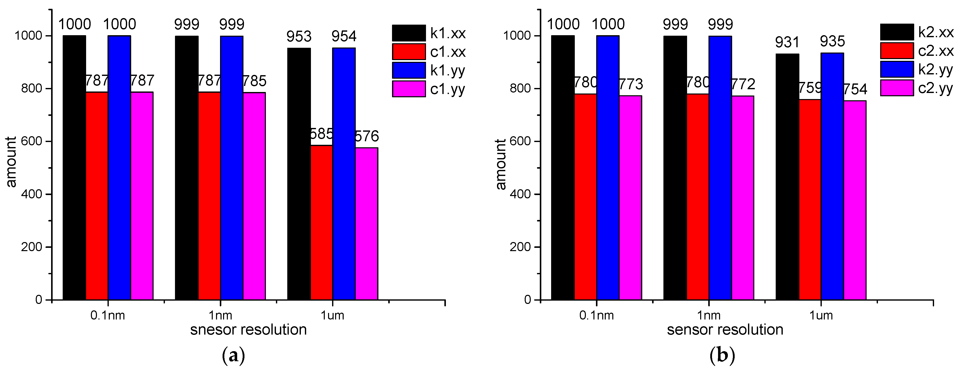
3.4.2. Discussion
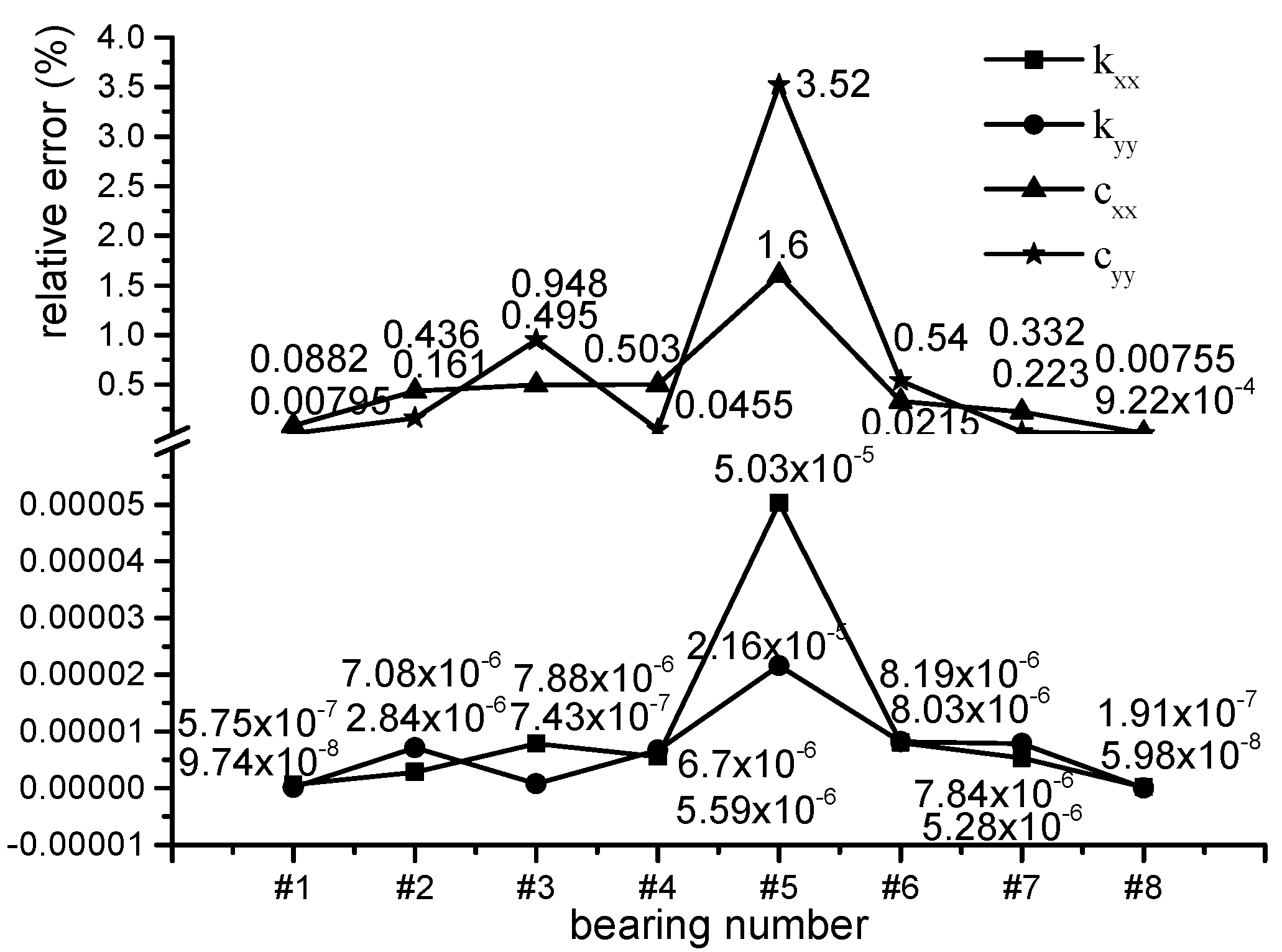
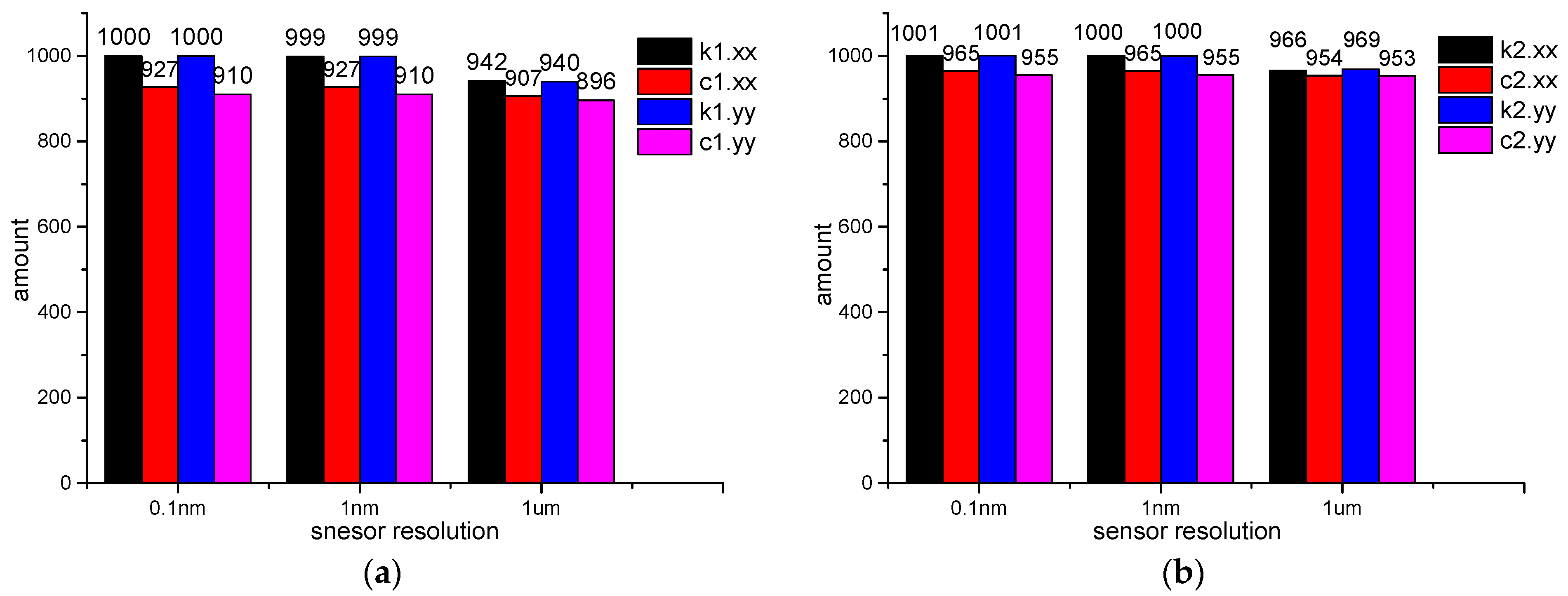
- (1)
- The numbers of LEFPs of the main stiffness coefficients are bigger than those of the main damping coefficients. It is indicated that the main stiffness coefficients of rolling bearings can be better identified than the main damping coefficients.
- (2)
- The amounts of LEFPs decrease when the sensor resolution is reduced. Only several stiffness coefficients’ relative errors are bigger than 10% when the sensor resolution is 0.1 nm. However, when the sensor resolution is 1 um, nearly half of the frequency points at which the stiffness coefficients’ relative errors are bigger than 10% in the simulation of g4.4.
- (3)
- When the sensor resolution is 0.1 nm, there are only dozens of, even zero LEFPs of the main stiffness coefficients in the simulation of g4.4. It is indicated that the stiffness bearing can be well identified by Algorithm I when the sensor resolution is 0.1 nm. While for the main damping coefficients, the number of LEFPs is much less than those of the main stiffness coefficients, which indicates that the stiffness coefficients cannot be well-identified. However, the damping coefficients of rolling bearings are far less than the stiffness coefficients. Hence, the damping coefficients of rolling bearings can be considered as zero. Therefore, Algorithm I can be used for rolling bearing in a multi-span and multi-disc rolling bearing-rotor system when the resolution is 0.1 nm.
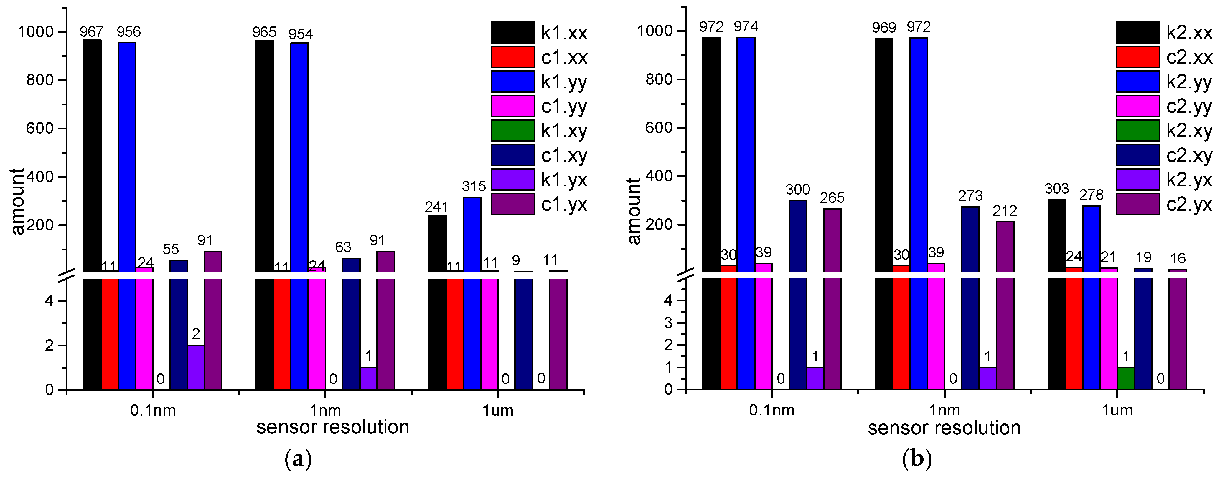
- (1)
- The numbers of LEFPs of the main stiffness coefficients are far greater than those of the main damping coefficients and the cross-coupled stiffness and damping coefficients. Hence, the main stiffness coefficients of rolling bearings can be better identified than the other coefficients. The reason is also that there is a very big difference between the main stiffness coefficients and the other coefficients of rolling bearings.
- (2)
- The amounts of LEFPs decrease when the sensor resolution is reduced. In the computational example g4.4, when the sensor resolution is 0.1 nm, there is less than half of the LEFPs of the main stiffness coefficients of #3, #5 and #6 bearing. There are about seven hundred LEFPs of the main stiffness coefficients of #2, #4 and #8 bearing. There are about nine hundred LEFPs of the main stiffness coefficients of #1 and #7 bearing. When the resolution is 1 um, the number of LEFPs decreases to less than 100.
- (1)
- The numbers of LEFPs of the damping coefficients of journal bearings are bigger than those of the stiffness coefficients, which indicates that the damping coefficients of journal bearings can be better identified than the stiffness coefficients.
- (2)
- The amount of LEFPs decrease when the sensor resolution is reduced. In the computational example h4.4, when the sensor resolution is 0.1 nm, most relative errors of the damping coefficients are lower than 10%. When the sensor resolution is 1 um, the LEFPs decrease to less than 100. As for the stiffness coefficients, the number of LEFPs is much less than that of the damping coefficients. There are only several, even zero LEFPs of the stiffness coefficients in the simulation of h4.4. For journal bearings, it is necessary to identify the four stiffness coefficients and the four damping coefficients.
4. Conclusions
- (1)
- The proposed algorithms provide a technique by which the stiffness and damping coefficients of each bearing can be monitored online under operation conditions. To identify the coefficients of all bearings in a rotor with n bearings and m discs, there should be m + n + 1 measured unbalance responses in both x and y directions. Moreover, the unbalance responses of each bearing should be measured. Algorithm I is suitable for rolling bearing coefficient identification, while Algorithm II can be applied to estimating both rolling-bearing coefficients and oil-journal bearing coefficients. External excitations and test runs are not required for the two algorithms. However, it is necessary to change the rotating speed slightly when using Algorithm II.
- (2)
- Adjustment points play a critical role in improving the identification accuracy of the two algorithms. Numerical simulations indicate that the coefficients of the bearing, which the adjustment point is near, are accurately identified. While the identification errors of the bearing, from which the adjustment point is far away, are often very big. Hence, in order to identify all bearings’ coefficients accurately, there should be an adjustment point near each bearing.
- (3)
- Accuracy of the unbalance response measurement system is very important to the two algorithms. Numerical simulations indicate that if the measuring errors of all the required unbalance responses are zero or the same, the identification errors are almost equal to zero. It is indicated that the repeatability precision of each measuring channel of the unbalance response measurement system plays a key role when using the two algorithms. Moreover, the two algorithms require high sensor resolution. The sensor resolution is higher, and the estimation accuracy is higher. Sensors with a resolution of 1 um should be avoided and sensors with a resolution of 0.1 nm are recommended for practical application.
Author Contributions
Funding
Institutional Review Board Statement
Informed Consent Statement
Data Availability Statement
Conflicts of Interest
Appendix A
- (1)
- Simulation of g1.4.


- (2)
- Simulation of g1.1.


Appendix B
- (1)
- Simulation of g1.4.

- (2)
- Simulation of g1.1.

Appendix C
- (1)
- Simulation of h1.4.

- (2)
- Simulation of h1.1

References
- Chen, W. A Simplified Identification Method of Dynamic Stiffness for the Heavy-Load and Low-Speed Journal Bearings. Teh. Vjesn. 2020, 27, 125–132. [Google Scholar]
- Kim, S.H.; Yeon, S.M.; Lee, J.H.; Kim, Y.W.; Lee, H.; Park, J. Additive manufacturing of a shift block via laser powder bed fusion: The simultaneous utilisation of optimised topology and a lattice structure. Virtual Phys. Prototyp. 2020, 15, 460–480. [Google Scholar] [CrossRef]
- Snyder, T.; Braun, M. Comparison of perturbed reynolds equation and cfd models for the prediction of dynamic coefficients of sliding bearings. Lubricants 2018, 6, 5. [Google Scholar] [CrossRef] [Green Version]
- Li, Q.; Zhang, S.; Ma, L.; Xu, W.; Zheng, S. Stiffness and damping coefficients for journal bearing using the 3D transient flow calculation. J. Mech. Sci. Technol. 2017, 31, 2083–2091. [Google Scholar] [CrossRef]
- Dyk, Š.; Rendl, J.; Byrtus, M.; Smolík, L. Dynamic coefficients and stability analysis of finite-length journal bearings considering approximate analytical solutions of the Reynolds equation. Tribol. Int. 2019, 130, 229–244. [Google Scholar] [CrossRef]
- Merelli, C.E.; Barilá, D.O.; Vignolo, G.G.; Quinzani, L.M. Dynamic coefficients of finite length journal bearing. Evaluation using a regular perturbation method. Int. J. Mech. Sci. 2019, 151, 251–262. [Google Scholar] [CrossRef] [Green Version]
- Kang, Y.; Shi, Z.; Zhang, H.; Zhen, D.; Gu, F. A novel method for the dynamic coefficients identification of journal bearings using Kalman filter. Sensors 2020, 20, 565. [Google Scholar] [CrossRef] [Green Version]
- Li, Q.; Wang, W.; Weaver, B.; Wood, H. Model-based interpolation-iteration method for bearing coefficients identification of operating flexible rotor-bearing system. Int. J. Mech. Sci. 2017, 131, 471–479. [Google Scholar] [CrossRef]
- Tiwari, R.; Lees, A.W.; Friswell, M.I. Identification of dynamic bearing parameters: A review. Shock. Vib. Dig. 2004, 36, 99–124. [Google Scholar] [CrossRef]
- Mutra, R.R. Identification of rotor bearing parameters using vibration response data in a turbocharger rotor. J. Comput. Appl. Res. Mech. Eng. 2019, 9, 145–156. [Google Scholar]
- Hagg, A.C.; Sankey, G.O. Some dynamic properties of oil-film journal bearings with reference to the unbalance vibration of rotors. J. Appl. Mech. 1956, 78, 302–306. [Google Scholar] [CrossRef]
- Duffin, S.; Johnson, B.T. Paper 4: Some Experimental and Theoretical Studies of Journal Bearings for Large Turbine-Generator Sets. In Proceedings of the Institution of Mechanical Engineers, London, UK, 1 June 1966. [Google Scholar]
- Tiwari, R.; Lees, A.W.; Friswell, M.I. Identification of speed-dependent bearing parameters. J. Sound Vib. 2002, 254, 967–986. [Google Scholar] [CrossRef] [Green Version]
- Tyminski, N.C.; Tuckmantel, F.W.; Cavalca, K.L.; de Castro, H.F. Bayesian inference applied to journal bearing parameter identification. J. Braz. Soc. Mech. Sci. Eng. 2017, 39, 2983–3004. [Google Scholar] [CrossRef]
- Chen, C.; Jing, J.; Cong, J.; Dai, Z. Identification of dynamic coefficients in circular journal bearings from unbalance response and complementary equations. Proc. Inst. Mech. Eng. Part J J. Eng. Tribol. 2019, 233, 1016–1028. [Google Scholar] [CrossRef]
- Song, Q.; Sun, F.; Ma, J. A New Algorithm and Experimental Investigation for the Identification of Dynamic Characteristics of Journal Bearings. J. Beijing Inst. Technol. 2002, 22, 682–686. [Google Scholar]
- Tiwari, R.; Chakravarthy, V. Identification of the bearing and unbalance parameters from rundown data of rotors. In IUTAM Symposium on Emerging Trends in Rotor Dynamics; Springer: Dordrecht, The Netherlands, 2011. [Google Scholar]
- Bently, D.E. Modal testing and parameter identification of rotating shaft/fluid lubricated bearing system. In Proceedings of the Fourth International Conference on Modal Analysis, Los Angeles, CA, USA, 3–6 February 1986. [Google Scholar]
- Stanway, R.; Tee, T.K.; Mottershead, J.E. Identification of squeeze-film bearing dynamics using a recursive, frequency-domain filter. In Proceedings of the ASME Twelfth Biennial Conference on Mechanical Vibration and Noise, Montreal, QC, Canada, 17–21 September 1989. [Google Scholar]
- Iida, H. Application of the Experimental Determination of Character Matrics to the Balancing of a Flexible Rotor. In Proceedings of the IFToMM 4th International Conference on Rotor Dynamics, Chicago, IL, USA, September 1994. [Google Scholar]
- Tiwari, R. Chakravarthy, V. Simultaneous identification of residual unbalances and bearing dynamic parameters from impulse responses of rotor–bearing systems. Mech. Syst. Signal Processing 2006, 20, 1590–1614. [Google Scholar] [CrossRef]
- Tiwari, R.; Chakravarthy, V. Simultaneous estimation of the residual unbalance and bearing dynamic parameters from the experimental data in a rotor-bearing system. Mech. Mach. Theory 2009, 44, 792–812. [Google Scholar] [CrossRef]
- Tiwari, R. Conditioning of regression matrices for simultaneous estimation of the residual unbalance and bearing dynamic parameters. Mech. Syst. Signal Processing 2005, 19, 1082–1095. [Google Scholar] [CrossRef]
- Wang, A.; Yao, W.; He, K.; Meng, G.; Cheng, X.; Yang, J. Analytical modelling and numerical experiment for simultaneous identification of unbalance and rolling-bearing coefficients of the continuous single-disc and single-span rotor-bearing system with Rayleigh beam model. Mech. Syst. Signal Processing 2019, 116, 322–346. [Google Scholar] [CrossRef]
- Wang, A.; Xia, Y.; Cheng, X.; Yang, J.; Meng, G. Continuous Rotor Dynamics of Multi-disc and Multi-span Rotor: Theoretical and Numerical Investigation on Continuous Model and Analytical Solution for Unbalance Responses. Appl. Sci. 2022. accepted. [Google Scholar]
- Wang, A.; Feng, Y.; Yang, J.; Cheng, X.; Meng, G. Continuous Rotor Dynamics of Multi-disc and Multi-span Rotor: A Theoretical and Numerical Investigation on Identification of Rotor Unbalance from Unbalance Responses. Appl. Sci. 2022, 12, 3865. [Google Scholar] [CrossRef]
- Wang, A.; Yao, W. Theoretical and Numerical Studies on Simultaneous Identification of Rotor Unbalance and Sixteen Dynamic Coefficients of Two Bearings Considering Unbalance Responses. Int. J. Control. Autom. Systems 2021. accepted. [Google Scholar]


| #14 | #29 | #33 | #49 | #53 | #69 | #73 | #91 |
| #14 | #29 | #31 | #49 | #51 | #69 | #71 | #89 |
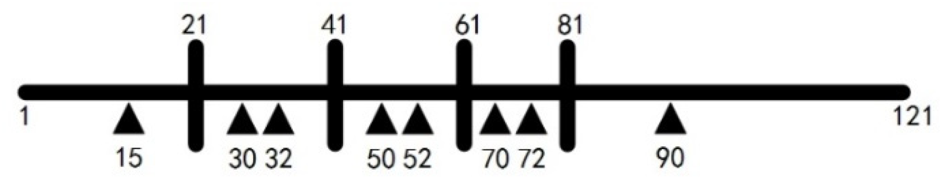
| The m + n measuring points | #15 (#1 bearing) | #90 (#2 bearing) | #61 (#disc) |
| Adjustment point | #14 | #91 |
| The m + n measuring points | #15 (#1 bearing) | #90 (#2 bearing) | #21 (disc) | #41 (disc) | #61 (disc) | #81 (disc) |
| Adjustment point | #14 | #91 |
| Relative error (%) | k1.xx | k2.xx | c1.xx | c2.xx | k1.yy | k2.yy | c1.yy | c2.yy |
| 2.706 × 10⁻⁷ | 6.16 × 10⁻⁸ | 0.0306 | 0.00977 | 2.39 × 10⁻⁷ | 8.162 × 10⁻⁸ | 0.141 | 0.0175 |
| Relative error (%) | k1.xx | k2.xx | c1.xx | c2.xx | k1.yy | k2.yy | c1.yy | c2.yy |
| 4.11 × 10⁻⁷ | 8.13 × 10⁻⁸ | 0.0227 | 0.00204 | 1.24 × 10⁻⁷ | 5.31 × 10⁻⁸ | 0.0130 | 0.00834 |
| The m + n measuring points | #3 (#1 bearing) | #47 (#2 bearing) | #31 (#disc) |
| Adjustment point | #2 | #48 |
| The m + n measuring points | #3 (#1 bearing) | #47 (#2 bearing) | #21 (disc) | #41 (disc) | #61 (disc) | #81 (disc) |
| Adjustment point | #2 | #48 |
| Relative error (%) | k1.xx | k2.xx | c1.xx | c2.xx | k1.yy | k2.yy | c1.yy | c2.yy |
| 3.25 × 10⁻⁷ | 6.00 × 10⁻⁷ | 0.00573 | 0.00192 | 3.11 × 10⁻⁷ | 5.63 × 10⁻⁷ | 0.0287 | 0.00352 | |
| Identified absolute value | k1.xy | k2.xy | c1.xy | c2.xy | k1.yx | k2.yx | c1.yx | c2.yx |
| 0.0333 | 0.0108 | 0.00998 | 0.00108 | 0.117 | 0.0159 | 0.00888 | 0.00155 |
| Relative error (%) | k1.xx | k2.xx | c1.xx | c2.xx | k1.yy | k2.yy | c1.yy | c2.yy |
| 4.94 × 10⁻⁷ | 1.85 × 10⁻⁷ | 0.00472 | 0.000425 | 2.22 × 10⁻⁷ | 9.48 × 10⁻⁸ | 0.00278 | 0.00170 | |
| Identified absolute value | k1.xy | k2.xy | c1.xy | c2.xy | k1.yx | k2.yx | c1.yx | c2.yx |
| 0.0210 | 0.00870 | 0.0154 | 0.00145 | 0.0108 | 0.00762 | 0.00480 | 0.000967 |
| Relative error (%) | k1.xx | k2.xx | k1.yy | k2.yy | k1.xy | k2.xy | k1.yx | k2.yx |
| 0.00435 | 0.00350 | 0.00537 | 0.0118 | 0.0324 | 0.0218 | 0.00346 | 0.00633 | |
| Relative error (%) | c1.xx | c2.xx | c1.yy | c2.yy | c1.xy | c2.xy | c1.yx | c2.yx |
| 1.56 × 10⁻⁵ | 0.000229 | 2.45 × 10⁻⁵ | 0.000204 | 0.000416 | 0.000188 | 9.41 × 10⁻⁵ | 0.000190 |
| Relative error (%) | k1.xx | k2.xx | k1.yy | k2.yy | k1.xy | k2.xy | k1.yx | k2.yx |
| 0.0535 | 0.0367 | 0.0184 | 0.181 | 0.677 | 0.241 | 0.0131 | 0.0879 | |
| Relative error (%) | c1.xx | c2.xx | c1.yy | c2.yy | c1.xy | c2.xy | c1.yx | c2.yx |
| 0.000281 | 0.000627 | 0.000152 | 0.000612 | 0.00926 | 0.000473 | 0.000265 | 0.000604 |
| Relative error (%) | k1.xx | k2.xx | c1.xx | c2.xx | k1.yy | k2.yy | c1.yy | c2.yy |
| 4.11 × 10⁻⁷ | 8.13 × 10⁻⁸ | 0.0227 | 0.00204 | 1.24 × 10⁻⁷ | 5.31 × 10⁻⁸ | 0.0130 | 0.00834 |
| Relative error (%) | k1.xx | k2.xx | c1.xx | c2.xx | k1.yy | k2.yy | c1.yy | c2.yy |
| 2.71 × 10⁻⁷ | 6.16 × 10⁻⁸ | 0.0306 | 0.00977 | 2.39 × 10⁻⁷ | 8.16 × 10⁻⁸ | 0.141 | 0.0175 |
| Relative error (%) | k1.xx | k2.xx | c1.xx | c2.xx | k1.yy | k2.yy | c1.yy | c2.yy |
| 4.94 × 10⁻⁷ | 1.11 × 10⁻⁷ | 0.00472 | 0.000425 | 1.51 × 10⁻⁷ | 9.51 × 10⁻⁸ | 0.00278 | 0.00170 | |
| Identified absolute value | k1.xy | k2.xy | c1.xy | c2.xy | k1.yx | k2.yx | c1.yx | c2.yx |
| 0.0210 | 0.00870 | 0.0154 | 0.00145 | 0.0108 | 0.00762 | 0.00480 | 0.000967 |
| Relative error (%) | k1.xx | k2.xx | c1.xx | c2.xx | k1.yy | k2.yy | c1.yy | c2.yy |
| 3.25 × 10⁻⁷ | 1.70 × 10⁻⁷ | 0.00573 | 0.00192 | 3.12 × 10⁻⁷ | 5.40 × 10⁻⁷ | 0.0287 | 0.00352 | |
| Identified absolute value | k1.xy | k2.xy | c1.xy | c2.xy | k1.yx | k2.yx | c1.yx | c2.yx |
| 0.0333 | 0.0108 | 0.00998 | 0.00108 | 0.117 | 0.0159 | 0.00888 | 0.00155 |
| Relative error (%) | k1.xx | k2.xx | c1.xx | c2.xx | k1.yy | k2.yy | c1.yy | c2.yy |
| 0.0535 | 0.0373 | 0.000281 | 0.000620 | 0.0184 | 0.182 | 0.000152 | 0.000618 | |
| Relative error (%) | k1.xy | k2.xy | c1.xy | c2.xy | k1.yx | k2.yx | c1.yx | c2.yx |
| 0.677 | 0.2494 | 0.00926 | 0.000472 | 0.0131 | 0.0857 | 0.000265 | 0.000627 |
| Relative error (%) | k1.xx | k2.xx | c1.xx | c2.xx | k1.yy | k2.yy | c1.yy | c2.yy |
| 0.00435 | 0.00350 | 1.56 × 10⁻⁵ | 0.000229 | 0.00537 | 0.0118 | 2.45 × 10⁻⁵ | 0.000204 | |
| Relative error (%) | k1.xy | k2.xy | c1.xy | c2.xy | k1.yx | k2.yx | c1.yx | c2.yx |
| 0.0324 | 0.0218 | 0.000416 | 0.000188 | 0.00345 | 0.00633 | 9.41 × 10⁻⁵ | 0.000190 |
Publisher’s Note: MDPI stays neutral with regard to jurisdictional claims in published maps and institutional affiliations. |
© 2022 by the authors. Licensee MDPI, Basel, Switzerland. This article is an open access article distributed under the terms and conditions of the Creative Commons Attribution (CC BY) license (https://creativecommons.org/licenses/by/4.0/).
Share and Cite
Wang, A.; Bi, Y.; Cheng, X.; Yang, J.; Meng, G.; Xia, Y.; Feng, Y. Continuous Rotor Dynamics of Multi-Disc and Multi-Span Rotor: A Theoretical and Numerical Investigation on the Identification of Bearing Coefficients from Unbalance Responses. Appl. Sci. 2022, 12, 4251. https://doi.org/10.3390/app12094251
Wang A, Bi Y, Cheng X, Yang J, Meng G, Xia Y, Feng Y. Continuous Rotor Dynamics of Multi-Disc and Multi-Span Rotor: A Theoretical and Numerical Investigation on the Identification of Bearing Coefficients from Unbalance Responses. Applied Sciences. 2022; 12(9):4251. https://doi.org/10.3390/app12094251
Chicago/Turabian StyleWang, Aiming, Yujie Bi, Xiaohan Cheng, Jie Yang, Guoying Meng, Yun Xia, and Yu Feng. 2022. "Continuous Rotor Dynamics of Multi-Disc and Multi-Span Rotor: A Theoretical and Numerical Investigation on the Identification of Bearing Coefficients from Unbalance Responses" Applied Sciences 12, no. 9: 4251. https://doi.org/10.3390/app12094251