
Dynamic Community Discovery Method Based on Phylogenetic Planted Partition in Temporal Networks


Abstract
:1. Introduction
1.1. Background
1.2. Motivation
1.3. Our Work and Contributes
- (1)
- The time dimension is introduced into the typical stochastic block-model, and all states in the whole dynamic network system are treated as variables, and the observation equation is taken as the constraint between variables to construct an error function about the whole dynamic network system.
- (2)
- By adopting the graph-based optimization strategy, the constraints in the entire motion trajectory can be considered once. In the linearization process, only the Jacobian matrix is calculated, and the calculation process is also relative to the entire motion trajectory. Therefore, the entire system evolution process is transformed into the nonlinear system optimization process.
- (3)
- In natural ecosystems, inspired by the evolutionary thinking of species populations and combined with the typical probability model of stochastic block-model in community discovery, a phylogenetic planted partition method (PPPM) for dynamic community discovery is proposed.
- (4)
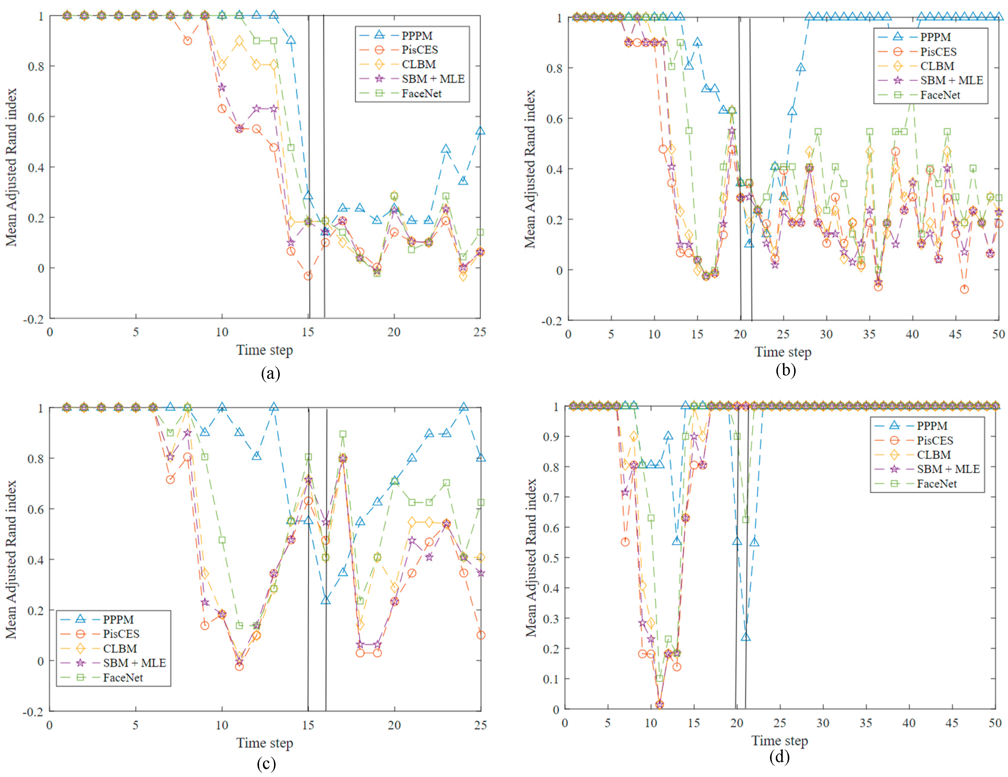
- The proposed PPPM method in the two scenarios of artificial network and the real network is verified by experiments, which proves that the performance of the novel method is better than the four state-of-the-art methods (FaceNet, SBM + MLE, CLBM, and PisCES).
1.4. Organization
2. Related Work
3. Meterials
3.1. Formal Definition
3.2. A Migration Partitioning Model for Phylogenetic Evolution
| Algorithm 1: Main procedure of the iterative method |
| 1. Given an initial value , radius and parameter k |
| 2. for the k-th iteration, solving: , s. t. |
| 3. Compute |
| 4. if |
| 5. |
| 6. else if |
| 7. |
| 8. |
| 9. if convergence |
| 10. break |
| 11. end |
| Algorithm 2: The main procedure of PPPM |
| Input:, k//dynamic networks and the number of communities Output://the community 1. at |
| 2. Initialize by using spectral clustering applied on |
| 3. at |
| 4. if iteration max iteration//hill-climbing algorithm |
| 5. //negative Log of the best adjacent case till to a constant |
| 6. //currently being traversing case |
| 7. for to do//traverse all adjacent solutions |
| 8. for to ; s.t. do |
| 9. //change community of a node |
| 10. compute using Equations (15)–(17) |
| 11. compute Log using (18) |
| 12. if then//current case is the best case |
| 13. |
| 14. //refresh community of current node |
| 15. if then//the best adjacent case is better than the current best case |
| 16. |
| 17. else//achieve a minimum |
| 18. break |
| 19. end |
| 20. end |
| 21. return |
4. Results
- (1)
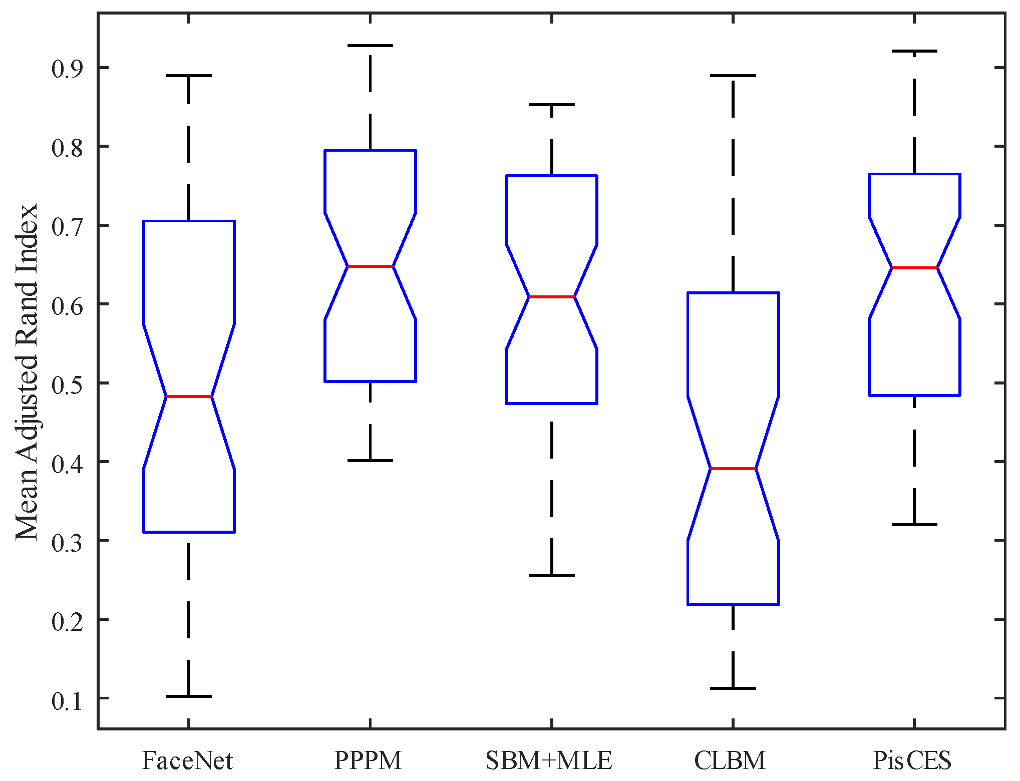
- Adjust Rand Index (ARI), , if the value of ARI is closer to 1, it means better results.where represents the expected value of and denotes the maximum value of .
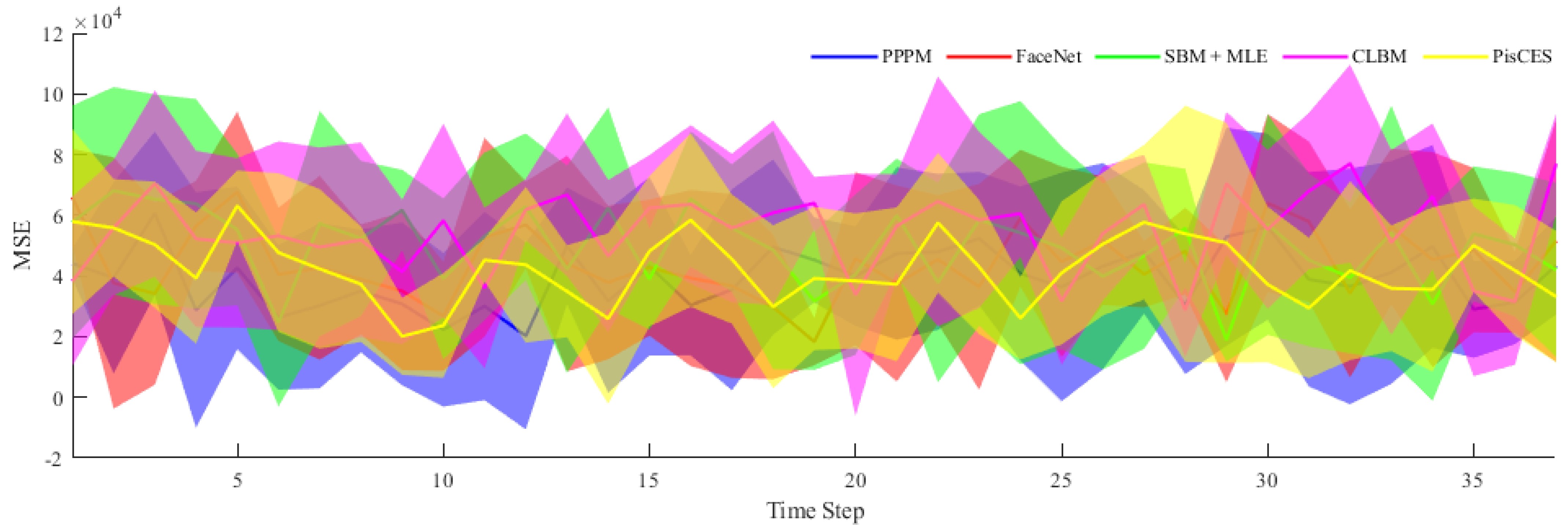
- (2)
- Mean-squared errors (MSE), the smaller the value, the smaller the error, that is, the better the result.where is the real data, expresses the fitting data, and implies the number of samples.
4.1. Synthetic Networks
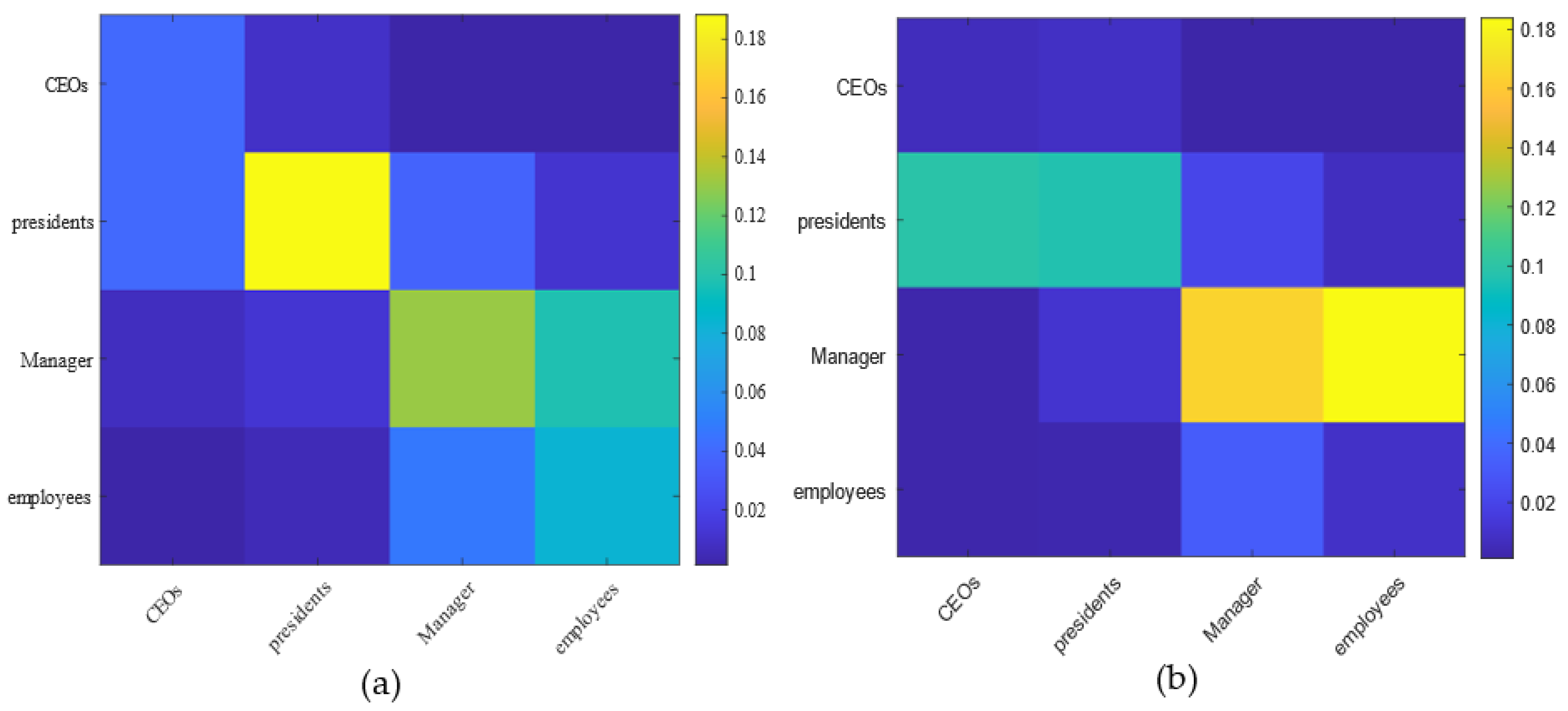
4.2. Real-World Networks
4.2.1. MIT Reality Mining
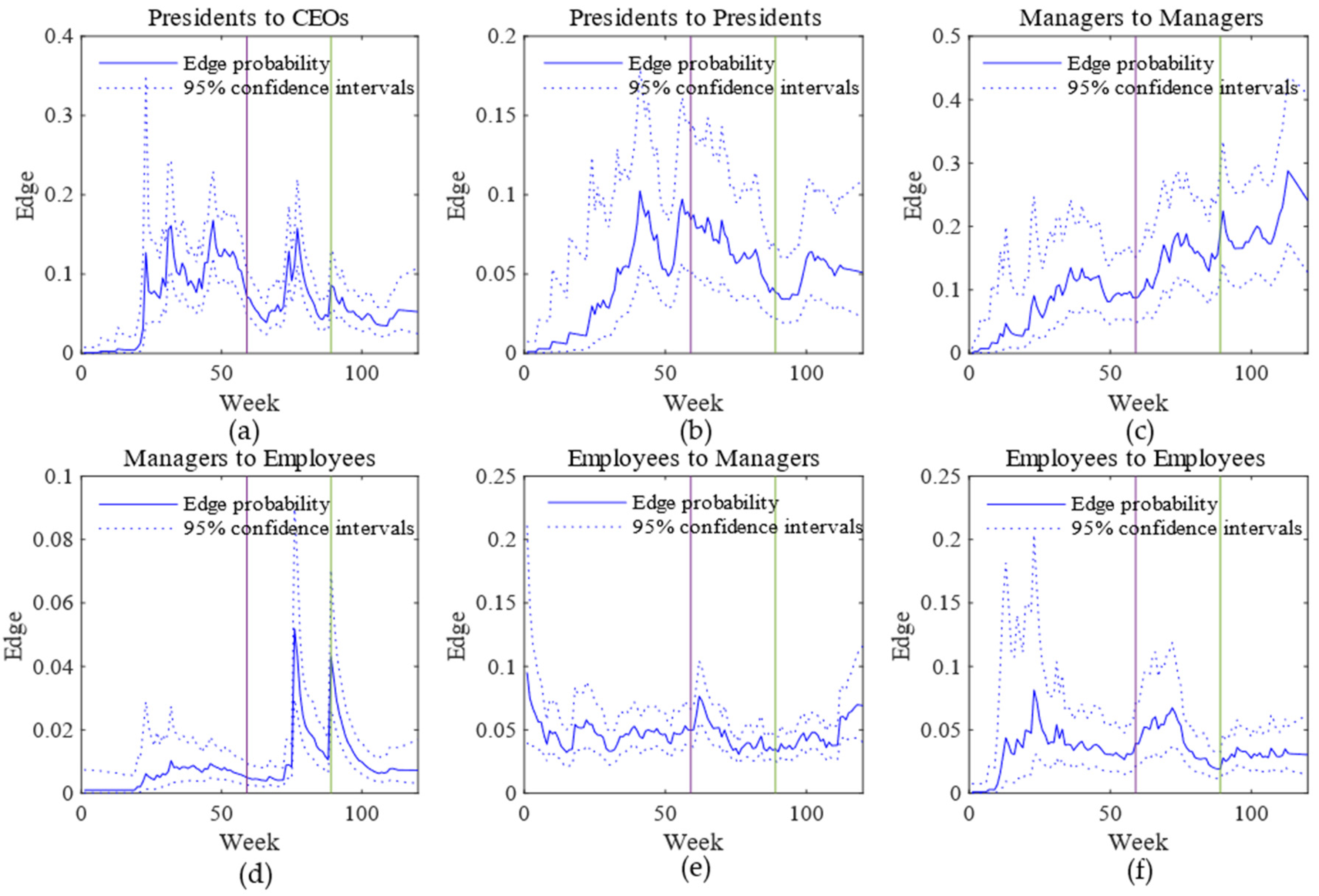
4.2.2. Enron Email Data
5. Conclusions
Author Contributions
Funding
Institutional Review Board Statement
Informed Consent Statement
Data Availability Statement
Conflicts of Interest
References
- Newman, M.E. The structure and function of complex networks. SIAM Rev. 2003, 45, 167–256. [Google Scholar] [CrossRef] [Green Version]
- Dakiche, N.; Benbouzid, F.T.; Slimani, Y.; Benatchba, K. Tracking community evolution in social networks: A survey. Inf. Process. Manag. 2018, 56, 1084–1102. [Google Scholar] [CrossRef]
- Girvan, M.; Newman, M.E. Community structure in social and biological networks. Proc. Natl. Acad. Sci. USA 2002, 99, 7821–7826. [Google Scholar] [CrossRef] [PubMed] [Green Version]
- Guruharsha, K.; Rual, J.F.; Zhai, B.; Mintseris, J.; Vaidya, P.; Vaidya, N.; Beekman, C.; Wong, C.; Rhee, D.Y.; Cenaj, O. A protein complex network of Drosophila melanogaster. Cell 2011, 147, 690–703. [Google Scholar] [CrossRef] [Green Version]
- Pagani, G.A.; Aiello, M. The power grid as a complex network: A survey. Physica A 2013, 392, 2688–2700. [Google Scholar] [CrossRef] [Green Version]
- Sanchez, F.; Mina, M. Oncogenic signaling pathways in the cancer genome atlas. Cell 2018, 173, 321–337. [Google Scholar] [CrossRef] [Green Version]
- Baccaletti, S.; Bianconi, G.; Criado, R. The structure and dynamics of multilayer networks. Phys. Rep. 2010, 544, 1–122. [Google Scholar] [CrossRef] [Green Version]
- Ma, X.; Sun, P.; Zhang, Z. An integrative framework for protein interaction and methylation data to discover epigenetic modules, IEEE/ACM Trans. Comput. Biot. Bioinf. 2019, 16, 1855–1866. [Google Scholar]
- Ma, X.; Dong, D.; Wang, Q. Community detection in multi-layer networks using joint nonnegative matrix factorization. IEEE Trans. Knowl. Data Eng. 2019, 31, 273–286. [Google Scholar] [CrossRef]
- Huang, Z.; Rege, X. Detecting community in attributed networks by dynamically exploring node attributes and topological structure. Knowl. Based Syst. 2020, 196, 105760. [Google Scholar] [CrossRef]
- Džamić, D.; Aloise, D.; Mladenović, N. Ascent–descent variable neighborhood decomposition search for community detection by modularity maximization. Ann. Oper. Res. 2019, 272, 273–287. [Google Scholar] [CrossRef]
- Karrer, B.; Newman, M.E. Stochastic blockmodels and community structure in networks. Phys. Rev. E 2011, 83, 016107. [Google Scholar] [CrossRef] [PubMed] [Green Version]
- Wen, Y.M.; Huang, L.; Wang, C.D.; Lin, K.Y. Direction recovery in undirected social networks based on community structure and popularity. Inform. Sci. 2019, 473, 31–43. [Google Scholar] [CrossRef]
- He, D.; Feng, Z.; Jin, D.; Wang, X.; Zhang, W. Joint identification of network communities and semantics via integrative modeling of network topologies and node contents. In Proceedings of the Thirty-First AAAI Conference on Artificial Intelligence, San Francisco, CA, USA, 4–9 February 2017; pp. 116–124. [Google Scholar]
- Airoldi, E.M.; Blei, D.M.; Fienberg, S.E.; Xing, E.P. Mixed membership stochastic blockmodels. J. Mach. Learn. Res. 2008, 9, 1981–2014. [Google Scholar]
- Qiao, M.; Yu, J.; Bian, W.; Li, Q.; Tao, D. Improving Stochastic Block Models by Incorporating Power-Law Degree Characteristic; IJCAI: Melbourne, Australia, 2017; pp. 2620–2626. [Google Scholar]
- Fortunato, S. Community detection in graphs. Phys. Rep. 2010, 486, 75–174. [Google Scholar] [CrossRef] [Green Version]
- Fortunato, S.; Hric, D. Community detection in networks: A user guide. Phys. Rep. 2016, 659, 1–44. [Google Scholar] [CrossRef] [Green Version]
- Rand, D.; Christakis, N. Dynamic social networks promote cooperation in experiments with humans. Proc. Natl. Acad. Sci. USA 2011, 108, 19193–19198. [Google Scholar] [CrossRef] [Green Version]
- Chiang, A.; Massagie, J. Molecular basis of metastasis. N. Engl. J. Med. 2008, 359, 927–932. [Google Scholar] [CrossRef] [Green Version]
- Kim, M.; Han, J. A particle-and-density based evolutionary clustering method for dynamic networks. Proc. VLDB Endow. 2009, 2, 622–633. [Google Scholar] [CrossRef] [Green Version]
- Folino, F.; Pizzuti, C. An evolutionary multi-objective approach for community discovery in dynamic networks. IEEE Trans. Knowl. Data Eng. 2014, 26, 1838–1852. [Google Scholar] [CrossRef]
- Chi, Y.; Song, X.; Zhou, D.; Hino, K.; Tseng, B.L. On evolutionary spectral clustering. ACM Trans. Knowl. Data Discov. 2009, 3, 1–30. [Google Scholar] [CrossRef]
- Wang, L.; Rege, M. Low-rank kernel matrix factorization for large-scale evolutionary clustering. IEEE Trans. Knowl. Data Eng. 2012, 24, 1036–1050. [Google Scholar] [CrossRef]
- Ma, X.; Dong, D. Evolutionary nonnegative matrix factorization algorithms for community detection in dynamic networks. IEEE Trans. Knowl. Data Eng. 2017, 29, 1045–1058. [Google Scholar] [CrossRef]
- Ma, X.; Zhang, B.; Ma, C.; Ma, Z. Co-regularized Nonnegative Matrix Factorization for Evolving Community Detection in Dynamic Networks. Inf. Sci. 2020, 528, 265–279. [Google Scholar] [CrossRef]
- Lin, Y.; Zhu, S. Analyzing communities and their evolutions in dynamic social networks. ACM Trans. Knowl. Discov. Data 2009, 3, 1–31. [Google Scholar] [CrossRef]
- Yang, T.; Chi, Y. Detecting communities and their evolutions in dynamic social networks-a bayesian approach. Mach. Learn. 2011, 82, 157–189. [Google Scholar] [CrossRef] [Green Version]
- Palla, G.; Barabási, A.L.; Vicsek, T. Quantifying social group evolution. Nature 2007, 446, 664–667. [Google Scholar] [CrossRef] [Green Version]
- Cazabet, R.; Amblard, F. Dynamic Community Detection. In Encyclopedia of Social Network Analysis and Mining; Springer: New York, NY, USA, 2014; pp. 404–414. [Google Scholar]
- Rossetti, G.; Cazabet, R. Community Discovery in Dynamic Networks: A Survey. ACM Comput. Surv. 2017, 51, 1–37. [Google Scholar] [CrossRef] [Green Version]
- Aynaud, T.; Fleury, E.; Guillarme. Communities in evolving networks: Definitions, detection, and analysis techniques. In Dynamics on and of Complex Networks; Springer: New York, NY, USA, 2013; Volume 2, pp. 159–200. [Google Scholar]
- Hartmann, T.; Kappes, A.; Wagner, D. Clustering Evolving Networks. In Algorithm Engineering; Springer: New York, NY, USA, 2016; Volume 9220, pp. 280–329. [Google Scholar]
- Agarwal, M.; Ramamritham, K.; Bhide, M. Real time discovery of dense clusters in highly dynamic graphs: Identifying real world events in highly. dynamic environments. Proc. VLDB Endow. 2012, 5, 980–991. [Google Scholar] [CrossRef]
- Tang, L.; Liu, H. Identifying evolving groups in dynamic multimode networks. IEEE Trans. Knowl. Data Eng. 2012, 24, 72–85. [Google Scholar] [CrossRef] [Green Version]
- Sun, J.; Faloutsos, C. Graphscope: Parameter-free of large time evolving-graph. In Proceedings of the 13th Conference on Knowledge Discovery Data Mining, New York, NY, USA, 12–15 August 2007; pp. 687–696. [Google Scholar]
- Chakrabarti, D.; Kumar, R.; Tomkins, A. Evolutionary clustering. In Proceedings of the 12th ACM SIGKDD International Conference on Knowledge Discovery and Data Mining, New York, NY, USA, 20–23 August 2006; pp. 554–560. [Google Scholar]
- Chi, Y.; Song, X.D.; Zhou, D.Y.; Koji, H.; Belle, L.T. Evolutionary spectral clustering by incorporating temporal smoothness. In Proceedings of the 13th ACM SIGKDD International Conference on Knowledge Discovery and Data Mining, New York, NY, USA, 12–15 August 2007; pp. 153–162. [Google Scholar]
- Folino, F.; Pizzuti, C. Multiobjective evolutionary community detection for dynamic networks. In Proceedings of the Conference on Genetic and Evolutionary Computation, Oregon, Portland, 7–11 July 2010; pp. 535–536. [Google Scholar]
- Gong, M.G.; Zhang, L.J.; Ma, J.J. Community detection in dynamic social networks based on multi-objective immune algorithm. J. Comput. Sci. Technol. 2012, 27, 455–467. [Google Scholar] [CrossRef]
- Xu, K.S.; Kliger, M.; Hero, A.O., III. Adaptive evolutionary clustering. Data Min. Knowl. Discov. 2014, 28, 304–336. [Google Scholar] [CrossRef] [Green Version]
- Han, Q.; Kevin, X.; Edoardo, A. Consistent estimation of dynamic and multilayer block models. In Proceedings of the 32th International Conference on Machine Learning, Lille, France, 6–11 July 2015; pp. 1511–1520. [Google Scholar]
- Kevin, X. Stochastic block transition models for dynamic networks. In Proceedings of the 18th International Conference on Artificial Intelligence and Statistics, San Diego, California, USA, 9–12 May 2015; pp. 1079–1087. [Google Scholar]
- Zhang, X.; Moore, C.; Newman, M.E.J. Random graph models for dynamic networks. Eur. Phys. J. B 2017, 90, 1–14. [Google Scholar] [CrossRef]
- Amir, G.; Pan, Z.; Aaron, C.; Cristopher, M.; Leto, P. Detectability Thresholds and Optimal Algorithms for Community Structure in Dynamic Networks. Phys. Rev. X 2016, 6, 031005. [Google Scholar]
- Sharmodeep, B.; Shirshendu, C. Spectral clustering for multiple dissociative sparse networks. arXiv 2017, arXiv:1805.10594. [Google Scholar]
- Paolo, B.; Fabrizio, L.; Piero, M.; Daniele, T. Detectability thresholds in networks with dynamic link and community structure. arXiv 2017, arXiv:1701.05804. [Google Scholar]
- Mehrnaz, A.; Theja, T. Block-Structure Based Time-Series Models for Graph Sequences. arXiv 2018, arXiv:1804.08796. [Google Scholar]
- Étienne, G.; Anthony, C.; Mustapha, L.; Hanane, A.; Loïc, G. Conditional Latent Block Model: A Multivariate Time Series Clustering Approach for Autonomous Driving Validation. arXiv 2020, arXiv:2008.00946. [Google Scholar]
- Emmanuel, A. Community Detection and Stochastic Block Models: Recent Developments. J. Mach. Learn. Res. 2017, 18, 1–86. [Google Scholar]
- Liu, F.; Choi, D. Global spectral clustering in dynamic networks. Proc. Natl. Acad. Sci. USA 2018, 115, 927–932. [Google Scholar] [CrossRef] [PubMed] [Green Version]
- Eagle, N.; Pentland, A.S.; Lazer, D. Inferring friendship network structure by using mobile phone data. Proc. Natl. Acad. Sci. USA 2009, 106, 15274–15278. [Google Scholar] [CrossRef] [PubMed] [Green Version]
- Klimt, B.; Yang, Y. The enron corpus: A new dataset for email classification research. In Proceedings of the European Conference on Machine Learning, Pisa, Italy, 20–24 September 2004; Springer: Berlin, Germany, 2004; pp. 217–226. [Google Scholar]


| Ref. | Year | Approach | Theory | Dataset |
|---|---|---|---|---|
| [42] | 2015 | Maximum Likelihood Estimation | Consistency | MIT Reality Mining |
| [43] | 2015 | Kalman Filtering + Local Search | / | Facebook wall posts |
| [44] | 2016 | Expectation Maximization | / | Internet AS graphs, Friendship networks |
| [45] | 2016 | Expectation Maximization | Detectability thresholds | Synthetic |
| [46] | 2017 | Expectation Maximization | Detectability thresholds | Synthetic |
| [47] | 2017 | Time-lag corrected | Convergence rates | Synthetic |
| [48] | 2018 | Aggregating SBM subroutines + MLE | Correctness/Stage-wise convergence rates | Enron emails, Facebook friendships |
| [49] | 2020 | Exhaustive grid search | Convergence rates | Synthetic |
| Our work | 2022 | Graph-based optimization | Convergence rates | MIT Reality Mining, Enron emails |
| Time Step | Random Rate | Proposed PPPM | PisCES | CLBM | SBM + MLE | FaceNet |
|---|---|---|---|---|---|---|
| 25 | 10% | 0.65702 | 0.50409 | 0.48838 | 0.56099 | 0.46667 |
| 50 | 0.56630 | 0.38265 | 0.34544 | 0.49414 | 0.34324 | |
| 25 | 20% | 0.72236 | 0.57972 | 0.54694 | 0.66961 | 0.50949 |
| 50 | 0.94401 | 0.90616 | 0.89504 | 0.92753 | 0.88592 | |
| Mean | 0.72242 | 0.670 | 0.56895 | 0.663068 | 0.55133 | |
| FaceNet | PPPM | SBM + MLE | CLBM | PisCES | |
|---|---|---|---|---|---|
| Max | 0.8991 | 0.9555 | 0.8678 | 0.8876 | 0.9412 |
| 75% | 0.7125 | 0.8005 | 0.7856 | 0.6258 | 0.7811 |
| Median | 0.4902 | 0.6523 | 0.6215 | 0.4981 | 0.6536 |
| 25% | 0.3154 | 0.5111 | 0.4992 | 0.2314 | 0.4902 |
| Min | 0.1002 | 0.40 | 0.2671 | 0.1487 | 0.3243 |
Publisher’s Note: MDPI stays neutral with regard to jurisdictional claims in published maps and institutional affiliations. |
© 2022 by the authors. Licensee MDPI, Basel, Switzerland. This article is an open access article distributed under the terms and conditions of the Creative Commons Attribution (CC BY) license (https://creativecommons.org/licenses/by/4.0/).
Share and Cite
Liu, X.; Ding, N.; Fiumara, G.; De Meo, P.; Ficara, A. Dynamic Community Discovery Method Based on Phylogenetic Planted Partition in Temporal Networks. Appl. Sci. 2022, 12, 3795. https://doi.org/10.3390/app12083795
Liu X, Ding N, Fiumara G, De Meo P, Ficara A. Dynamic Community Discovery Method Based on Phylogenetic Planted Partition in Temporal Networks. Applied Sciences. 2022; 12(8):3795. https://doi.org/10.3390/app12083795
Chicago/Turabian StyleLiu, Xiaoyang, Nan Ding, Giacomo Fiumara, Pasquale De Meo, and Annamaria Ficara. 2022. "Dynamic Community Discovery Method Based on Phylogenetic Planted Partition in Temporal Networks" Applied Sciences 12, no. 8: 3795. https://doi.org/10.3390/app12083795