Monocular Real Time Full Resolution Depth Estimation Arrangement with a Tunable Lens

Abstract

This work introduces a real-time full-resolution depth estimation device, which allows integral displays to be fed with a real-time light-field. The core principle of the technique is a high-speed focal stack acquisition method combined with an efficient implementation of the depth estimation algorithm, allowing the generation of real time, high resolution depth maps. As the procedure does not depend on any custom hardware, if the requirements are met, the described method can turn any high speed camera into a 3D camera with true depth output. The concept was tested with an experimental setup consisting of an electronically variable focus lens, a high-speed camera, and a GPU for processing, plus a control board for lens and image sensor synchronization. The comparison with other state of the art algorithms shows our advantages in computational time and precision.

1. Introduction

Standard cameras can extract 2D light information from a scene, which includes intensity and wavelength. However, 3D details are lost during this process due to lack of information regarding the direction of each ray of light. The 3D data is essential to a better understanding of the scene as it could be used to find the placement of objects more accurately in the scene [1,2], or to construct 3D mesh [3,4,5,6], or for artistic purposes in disciplines such as cinematography or computer game development [7].

Several methods exist that obtain 3D volumes. They can be classified in two main groups: active or passive. While active methods require additional hardware that emits light information from the device to sense the 3D information of the scene [7,8,9,10,11], passive methods use only the received light information. Classical passive methods consist of utilizing stereo [12,13,14], structure from motion (SFM) [15,16,17], depth from focus (DFF) [18,19] or approaches with a monocular camera and single images using deep learning techniques [20,21]. Passive methods usually do not allow obtaining the 3D information in real time, as they require a high level of computational processing, and the single capture approach cannot obtain real distances.

The vision system presented in this paper extracts 3D information in real time using a sensor coupled with a variable focus lens, obtaining a full pipeline for passive real time 3D extraction. A comparison with other widespread methods yields that our algorithm is faster and more accurate.

2. Materials and Methods

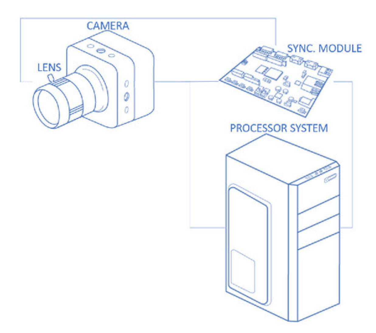
Our proposal is a vision system setup to capture 3D images in real time. There are two main components to ensure the full pipeline, the setup (Hardware components) and the algorithm (Software component). Both are described in the next sections.

2.1. Setup

2.1.1. General Overview

To achieve the hardware part of our vision system, several components were selected (Figure 1): a variable focus lens, a high speed camera, a synchronization module and a processing system.

A liquid lens was chosen as a variable focus lens. Due to the capability of fast movement, the fastest in the market is capable of moving at least 156 fps with high precision and repeatability. The camera captures Full HD ($1920\times 1080$) with a high frame rate (greater than 156), and supports the lens mount (C-mount). As a synchronization module, we use a microprocessor to synchronize the lens and the camera with high accuracy, to this purpose, an FPGA was selected, since the FPGAs allow to generate multiple clocks without losing cycles. Finally, the processing system must support reading all the camera frames and needs a GPU that executes the parallel algorithm.

Our algorithm is capable of extracting the distances from the captured frames, estimating distances with high accuracy, and dealing with the low frequencies problem by using the input color information, a common issue in DFF algorithms [22].

2.1.2. Camera

The camera requirements need to be chosen according to the selected optics and to the desired resolution of the depth information. In the setup used for this paper, the variable focus lens is C-mount. The lens acquires six different focus planes by sweeping from the nearest focus to the farthest focus (infinity) without an overlapping depth of field. The camera must be C-mount compatible and have at least a frame rate of 150 frames per second (fps) to simulate a real time 25 fps camera. Using a global shutter is mandatory to avoid artifacts while capturing at high frame rate speed. Additionally, an Opto-isolated trigger input/output is needed to perform the correct synchronization with the lens and a high-speed interface for data transfer. To send this amount of data, at least a 3 Gb/s speed bus is needed using Bayer pattern following Equation (1):

$$AD=\frac{F\times W\times H\times C\times 8}{{1024}^3}$$

(1)

where $AD$ is the amount of data in Gb/s, F the number of frames per second and W, H, C are width, height, and channels, respectively. Usable interfaces that can transfer such high amounts of data are, but not limited to, the Camera Link (CL), CoaXPress (CXP) and MIPI, depending on the version and lanes. For the setup used in the camera presented here, a frame grabber was used to read the output data. The camera and frame grabber used in this setup are the Flare2MP [23] and Matrox Radient eV-CL [24]. The capture is done at 156 fps with an exposure time of 6 milliseconds.

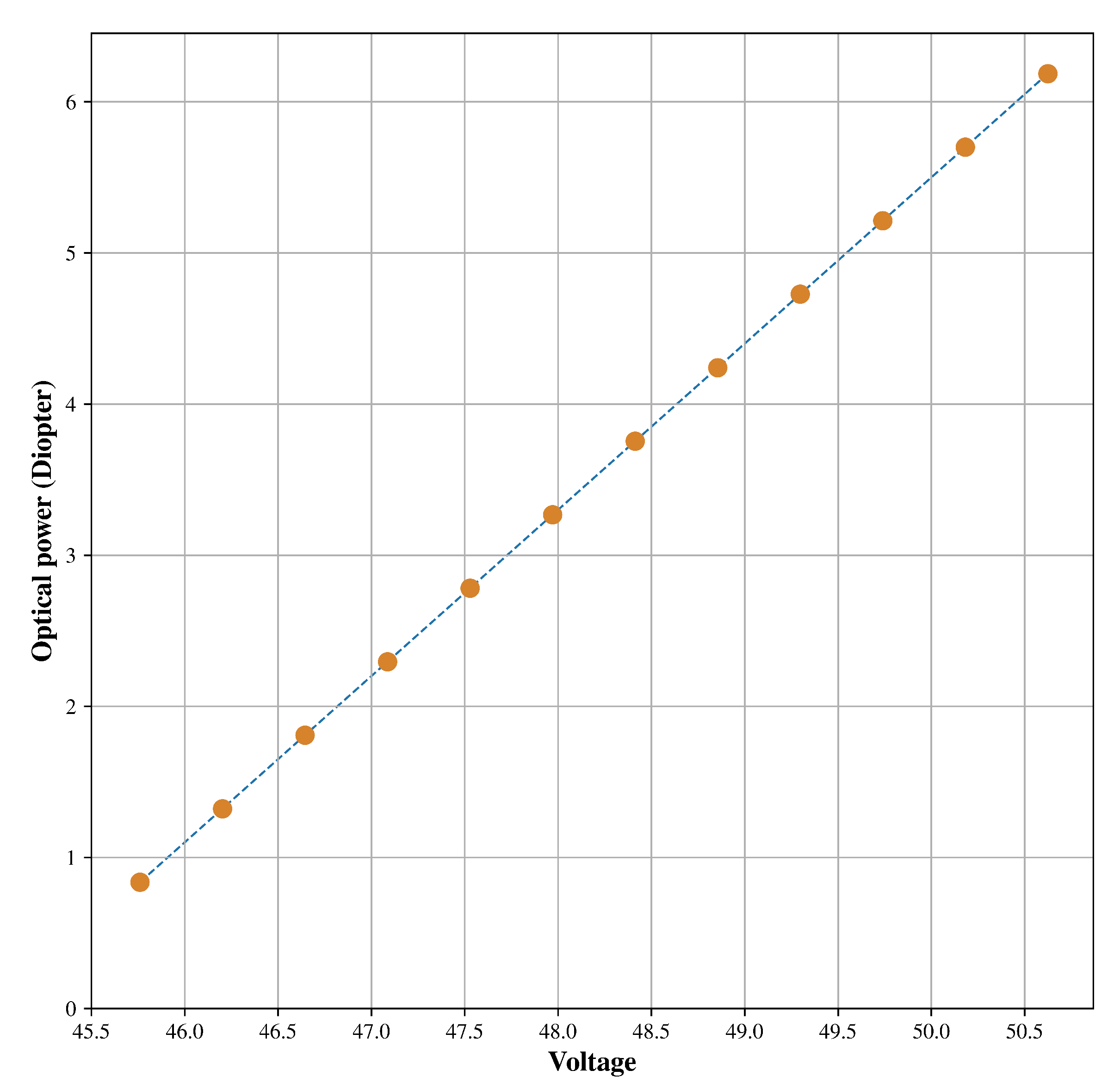
2.1.3. Variable Focus Lens

In order to capture multiple images of the same scene at different focus positions at high speed, a variable focus lens is needed. In our setup, an electronically focus controllable lens is used (Varioptic’s C-C-39N0-250) [25].

This lens is controlled using a custom-made camera-lens synchronization module using an FPGA that accurately controls the lens focus distance with the image sensor trigger, capturing the images in the focal stack. The focus sweep curve follows a “sawtooth” graph when plotted as focus time vs. total time from near to far focus. Between the near and far focus, six images with short exposure time are acquired, consuming a total time of 38.4 ms to capture one focal stack. This provides an effective frame rate of 26 fps (156 total frames acquired by the image sensor). Figure 2 shows the sawtooth described. In our case it is necessary to send two commands to the liquid lens to achieve focus repeatability by image captured, the Figure 3 displays the voltage rms values used to modifiy the focal-length as well as the optical power.

Liquid lenses have been successfully used in another fields, for example in the medical and surgical sectors by increasing the depth of field [26], or adding other kind of information as polarization to 3D scenes resulting in a 4 dimensions experimental space [27].

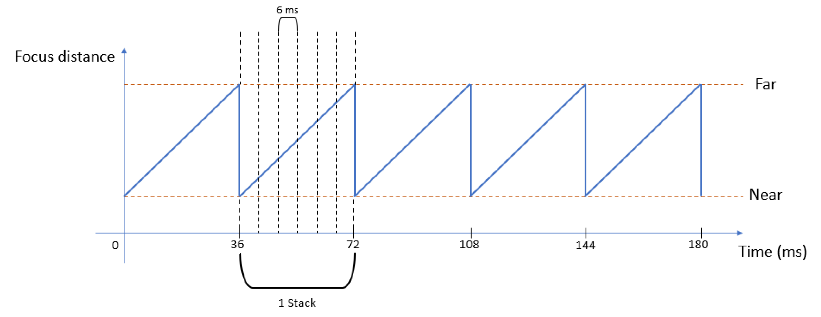
2.2. Synchronization Module

Camera, lens and system processors must be synchronized to obtain the focal stack in the desired moment without losing any cycle of CPU, however, common CPU’s are not valid due to clock uncertainty. To achieve the desired synchronization requirements, any microprocessor able to generate two clocks and an I2C signal is valid. An Arty Z7 [28] was chosen, using VHDL language to generate the properly modules to control the lens via I2C and generate output clocks to the trigger and the lens, using as input a PC reset to start capturing.

Processor System

Once the focal stack is captured, it is sent to the processing system to estimate depth. This system can be any hardware capable of processing and reading the incoming data at the needed speed. In the setup, the depth estimation algorithm (explained in Section 2.3) runs on a GeForce RTX 1080 GPU, and the data is transferred to the GPU using the Matrox Radient eV-CL already described.

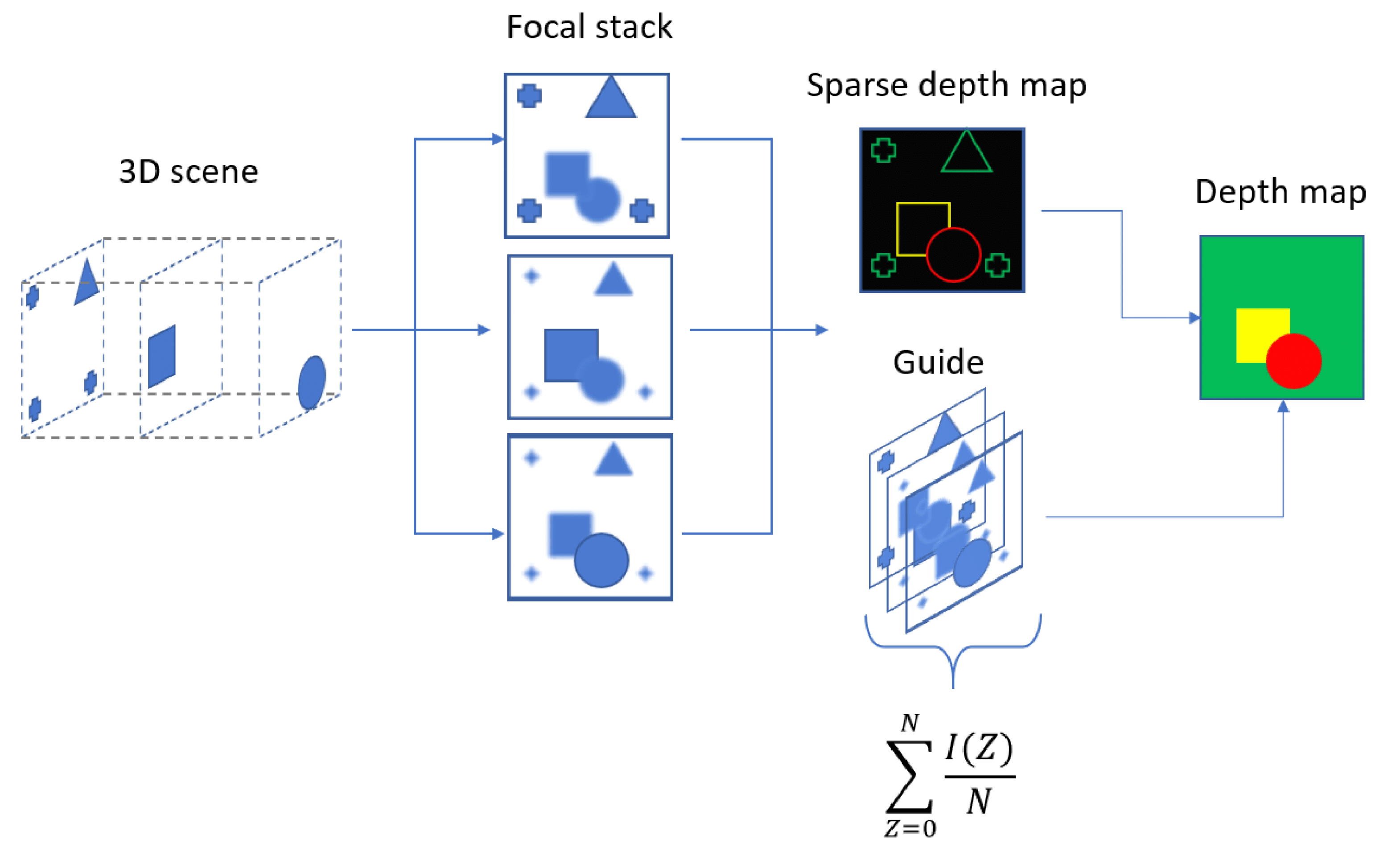
2.3. Depth Estimation Algorithm

Dense depth estimation algorithms must obtain the non textureless zones, and fill the textureless zones with the neighbour information, in this paper the result of obtaining the high frequency zones are defined as a sparse estimation of depth. The sparse estimation of depth is done by composing the focal stack using a defocus operator [29]. The amount of information estimated will heavily depend on the scene; if the image is lacking high frequencies, depth cannot be estimated. Once the sparse depth map has been computed, the unknown values must be filled. To this purpose, a sparse depth map and a composition of the focal stack is used as a starting point to fill the algorithm. Figure 4 below shows the steps in the algorithm pipeline.

Let $I\left(z\right)$ be the focal stack with shape $W\times H\times N$ with W, H, N as height, width and the number of planes of the stack, respectively, the sparse depth map is defined as follows:

$$SD=\underset{z}{max}G\left(I\right)\bigcap _{i=2}^n\underset{z}{max}\left(U_i\left(G\left(R_{\frac{1}{i}}\left(I\right)\right)\right)\right)$$

(2)

where $G_z\left(I\right)$ is the 2D gradient magnitude function for each image of the stack, $U_i$ is an area upsample function and $R_{\frac{1}{i}}$ is an area downsample function, where i is the factor to resize and n the maximum number of pyramids, for our results n value is equal to 3. The multiscale approach avoids noise artifacts due to the elimination of small noisy pixels, the maximum gradients that exceed a tolerance factor with respect to the other gradient values of the stack will be considered. As only gradients are used, the resulting sparse depth map will have information only along the edges. However, a complete depth map is needed. Figure 5 shows a real sparse depth map obtained with our camera.

The next step prior to generating a depth map is to evaluate the movement intra-stack, the idea of capture in non-static scenes generates artifacts due to the displacement occurred between each stack plane, the procedure is to eliminate the artifacts from the sparse depth-map using a Z-entropy function as named in the Equation (3), the regularization procedure does not enhance the movement because of the technique.

$$H\left(S\right)+\sum _z^{n}I\left(z\right){log}_{2}I\left(z\right)$$

(3)

where S is the stack, H the entropy and z is the index of each plane, to this procedure the input image is selected by bins, the idea is to have, at most, 2 bit to represent the different values in the same pixel along the z axis, avoiding big changes due to the movement.

Another part of the algorithm implies inferring the unknown values in the sparse depth map. The final solution should satisfy the following constraints:

• All the data points in the existing sparse depth map have to be present in the final solution.
• There are no missing depth values.
• The resulting depth map should be edge preserving and should be smooth within the map.

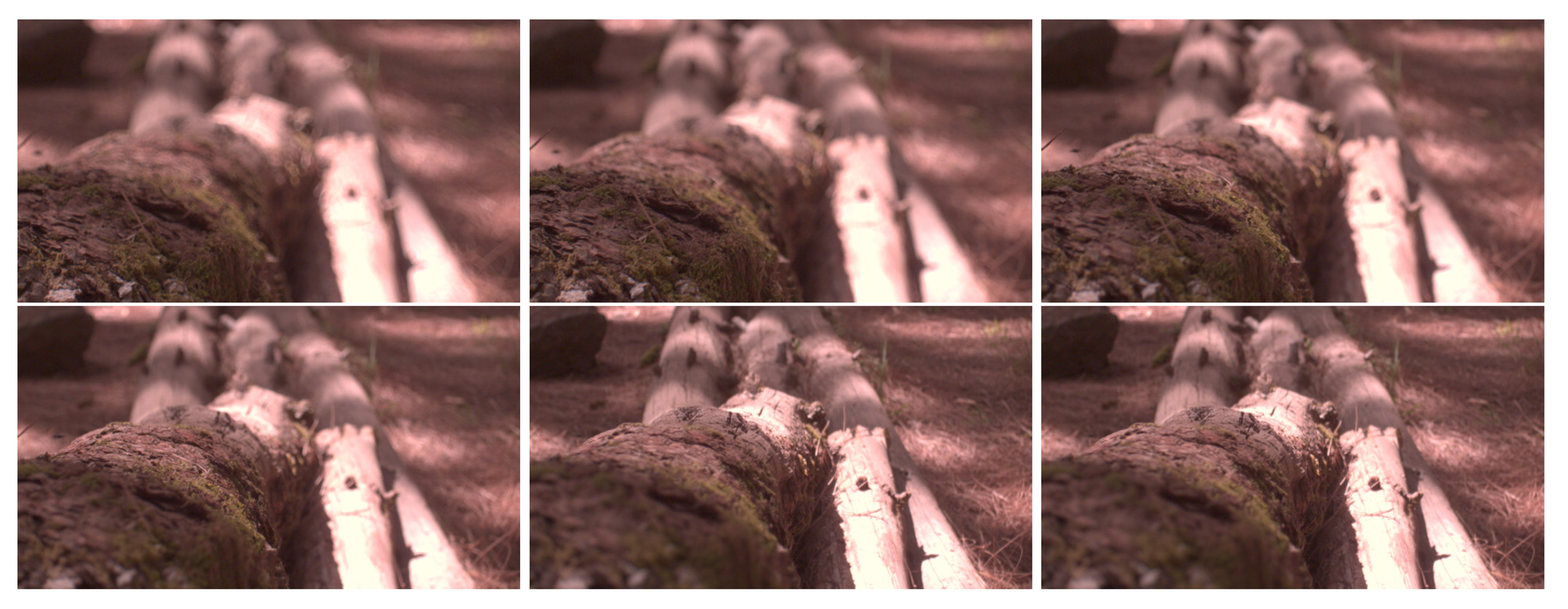
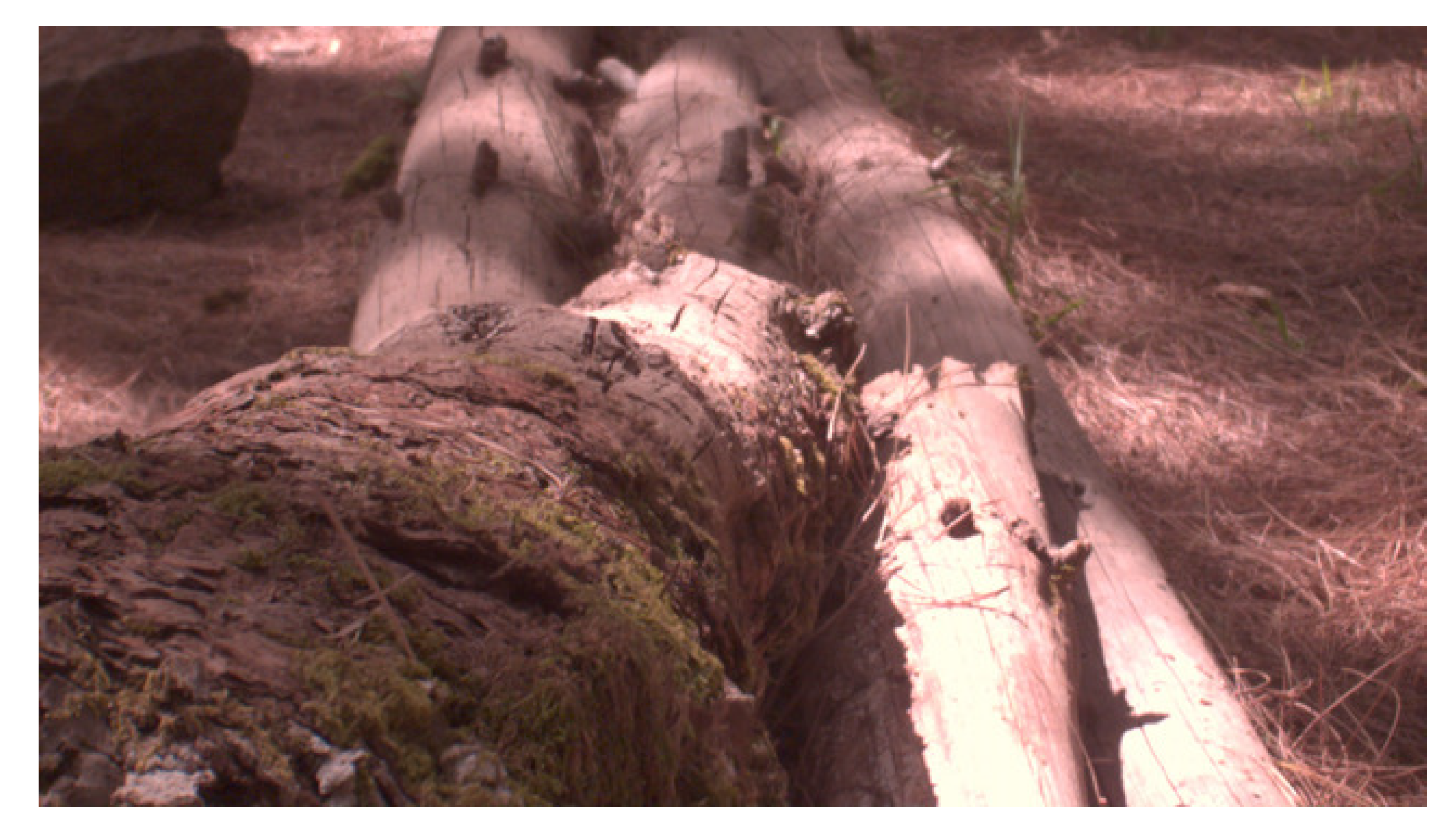
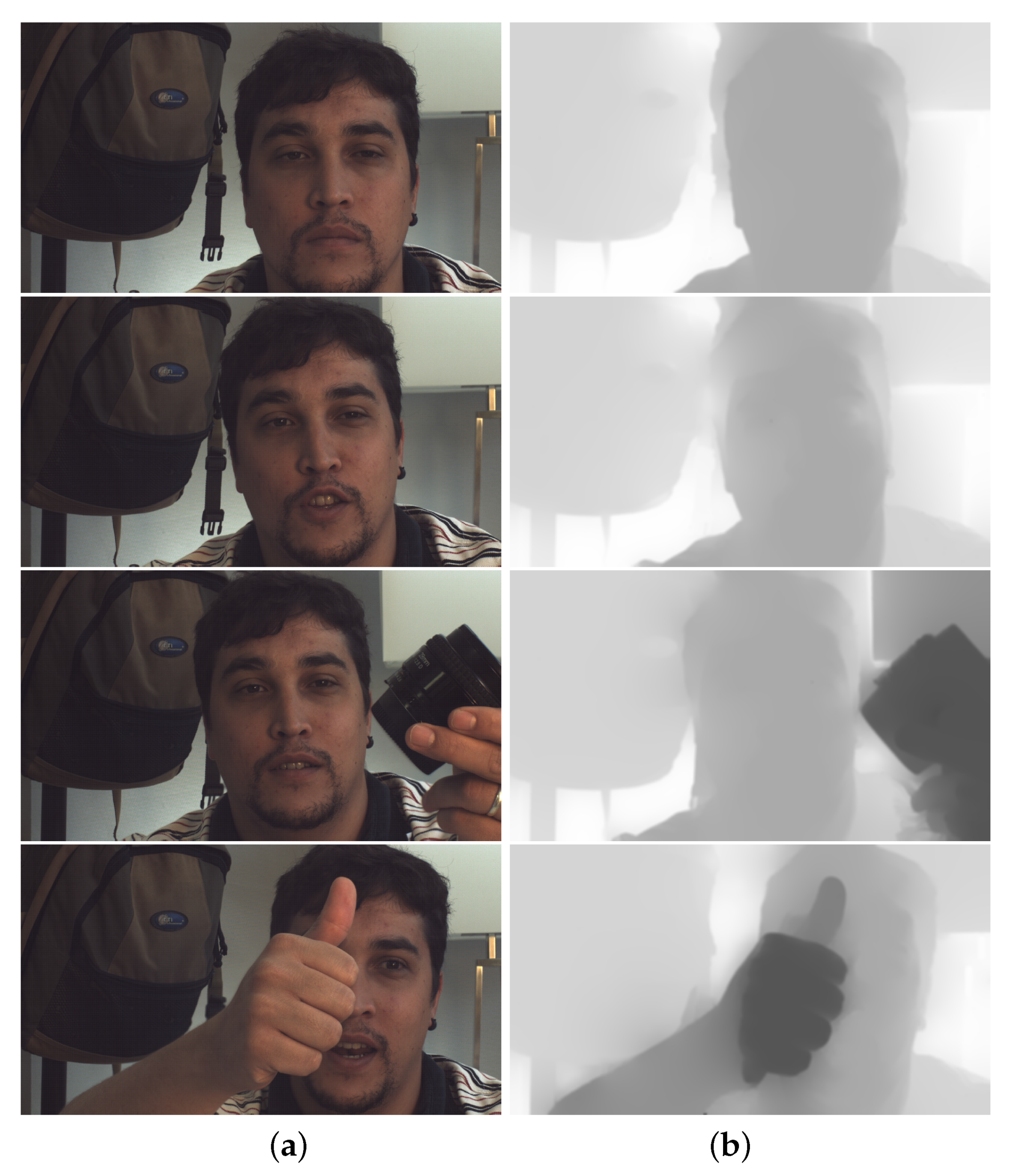
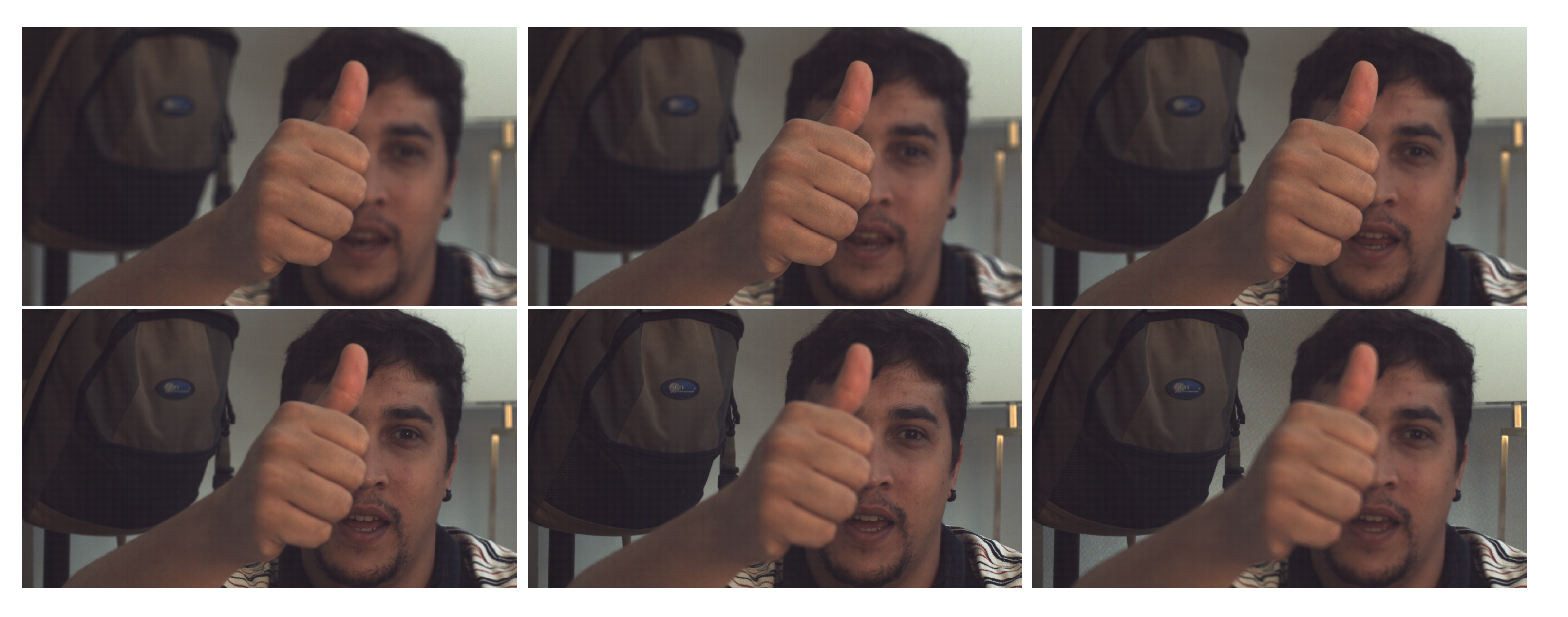
Following the previous statement, the solution will be the one that minimizes the error function:

$$\lambda S(D,R)+\sum _{x,y}M(x,y){(D(x,y)-SD(x,y))}^2$$

(4)

where $D(x,y)$ is the resulting depth map, $M(x,y)$ is the binary mask of Equation (5), this parameter ensures that the original values of the sparse depth-map are not modified and $S(D,R)$ is the smooth term weighted with the parameter $\lambda$ which ensures that the depth map is smooth at the same time that preserves the edges present in the reference R, the idea of $S(D,R)$ is to fill the depth map values using the sparse depth-map, which is the first iteration but also using the color distance provided by the reference.

$$M(x,y)=\left\{\begin{array}{cc}0\hfill & \mathrm{if}SD(x,y)\mathrm{is}\mathrm{uncertain}\hfill \\ 1,\hfill & \mathrm{else}\hfill \end{array}\right.$$

(5)

The reference R is a simple composition of the input stack presented in Equation (6) and the smoothing term defined by Equation (7).

$$R(x,y)=\sum _{z}I(x,y,z)/N$$

(6)

$$S(D,R)=\sum _{x_1,y_1,x_2,y_2}\widehat{W}(R,x_1,y_1,x_2,y_2){(D(x_1,y_1)-D(x_2,y_2))}^2$$

(7)

where $\widehat{W}(R,x_1,y_1,x_2,y_2)$ is the bistochastized version of a bilateral affinity function W. The affinity of each pixel depends not only on the distance between each other, but also in the color distance in the YUV color space. W is defined as follows:

$$\begin{array}{c}W(R,x_1,y_1,x_2,y_2)=\hfill \\ \hfill exp\left(-\frac{\parallel (x_1,y_1)-(x_2,y_2){\parallel }^2}{2{\sigma }_{xy}^2}-\frac{{(R_l(x_1,y_1)-R_l(x_2,y_2))}^2}{2{\sigma }_l^2}-\frac{\parallel R_{uv}(x_1,y_1)-R_{uv}(x_2,y_2){\parallel }^2}{2{\sigma }_{uv}^2}\right)\end{array}$$

(8)

where ${\sigma }_{xy}^2$, ${\sigma }_l^2$ and ${\sigma }_{uv}^2$ are the spatial, luma and uv variances, respectively.

The problem of minimizing the error function (4) is intractable; however, it can be modified as in [30,31] to solve the problem in bilateral space [32].

With the problem modified, the selected parameters to execute the algorithm are ${\sigma }_{xy}=16$, ${\sigma }_l=16$ and ${\sigma }_{uv}=16$, obtaining a grid of $16\times 16\times 16$ in the bilateral space, this reduces the number of neighbours in the search of candidates reducing the computational time, to remove the square artifacts produced by our approach, a final Gaussian blur is applied using a kernel size of $ks=16\times 1.2$ and a $\sigma =ks\times 0.7$ obtaining the result shown in Figure 6.

3. Results

This section presents the results of our arrangement. The working principle of our system is depth estimation from the focal stack acquired using a liquid lens.

The raw data obtained by our arrangement are presented in the Figure 7, by showing the images in the focal stack used to calculate the depth map shown in Figure 6. With the resulting depth map it is also possible to extract an All In Focus (AIF) image as shown in Figure 8, by using and interpolating the depth map indices with the input images.

Fast capture acquisition allows the intra-stack movement to be decreased, avoiding high frequencies artifacts in the depth map. Some frames extracted from a captured video are shown in the Figure 9. As discussed in Section 2.3, it is necessary to compute the Z-entropy to remove the movement artifacts, the Figure 10 presents a stack with some movement in the hand and in the mouse and the Figure 11 shows the mask detected as movement to remove from the sparse depth map.

Figure 12 shows a 3D point cloud that was generated using the depth map (Figure 6) and the all in focus (Figure 8) by using the intrinsics parameters of the camera to assign the Z distances.

4. Discussion

The experimental setup is not directly comparable with other methods of acquisition, in that way different algorithms are chosen to compare the depth maps results.

There are many different algorithms proposed in the state of the art to approximate the depth estimation from focal stack capture [19,22,34,35,36,37]. The discussion is presented by choosing three, with the first chosen due to the similarity of the capture system [34], Hui et al. presents a camera with a liquid lens which obtains the different focus positions varying the voltage like the arrangement proposed in this document. The second algorithm is the most referenced [36] in the literature, and uses classic computer vision to solve the problem, that is also comparable with the algorithm presented in the Section 2.3. The last one was selected to compare a classical computer vision algorithm with neural networks and is the first article that uses neural networks to solve the problem [19]. The article presented by our team [37] was compared visually with the algorithm presented here in the same way than the others. Noise study was not applied here given that the ground-truth used for this study were contemplated in the training stage.

In the method presented in this paper, the focal stack acquisition and processing is done in real time, allowing for live video as presented in Section 2.3. In addition, our prototype works outdoors even with direct sunlight from behind the objects. Figure 13 shows the comparison between the method presented in this paper and the methods mentioned before [19,34,36], using real images. Only the computer vision algorithm could be compared as the focal stack was obtained with our camera and we did not have access to the raw data collected in the referenced works.

In the images shown in Figure 13, our algorithm appears to be more edge preserving and smooth with the environment of the scene. Hui et al.’s implementation appears to work well with big objects inside the scene, the algorithm is edge preserving but not very smooth between the different levels of distances. The DDFF algorithm has very low resolution output, and the neural network is trained with a mobile captured dataset under very different conditions than the proposed cameras. VDFF and our results are similar but execute slower and has less accuracy under noisy conditions.

Relative multiscale deep depth from a focus approach [37] is compared with the same images as the others, as shown in the Figure 14. The neural network approach shows better results in some scenes. Under textureless zones, the zone without edges has good depth map values, but if we modify or use images of a camera with a different configuration, like the three top images, the classical algorithms adapt better than the neural network approach, and the same happens if we add a macro lens in the top of the arrangement and capture the focal stack by varying the focus positions, as we can see in the bottom images.

To evaluate the accuracy of our method a PSNR metric was chosen:

$$PSNR=10{log}_{10}\left(\frac{M^2}{MSE(D,GT)}\right),$$

(9)

where M is the maximum pixel value and $MSE$ is the mean squared error between D computed depth map and $GT$ ground truth. The metric result is expressed in dB. Ground truth depth maps were obtained from Middleburry dataset [39], using the original left image to generate synthetic defocused images following the procedure of J. Lee et al. [40]. The comparison shown in Figure 15 was made using different images of the cited dataset, by adding simulated camera noise to evaluate the robustness of the different algorithms. The PSNR average was computed with the following equation:

$$PSN{R}_A=10{log}_{10}\left(\frac{{\sum }_{i=0}^N{10}^{\frac{PSNR\left(D\right(i),GT(i\left)\right)}{10}}}{N}\right)$$

(10)

where N is the number of the images in the dataset, five in our case. Figure 16 shows some of the result over one image with the different methods and the ground truth.

Table 1. Comparison times for a 10 planes focal stack. The approach presented executes faster and with best accuracy than the compared methods.

Method	Runtime (ms)	PSNR Average (dB)
Ours	38	29.25
DDFF	580	22.01
Hui et al	3700	22.77
VDFF	7362	24.87

shows the average PSNR and the runtime comparison. These measurements use 10 planes due to the limitation of the DDFF algorithm. Comparison times of DDFF were extracted from their article, and the code is provided by the author. Hui et al was implemented in Python, using the paper explanation, and the times were extracted from their article, taking the time that they expose for one plane and multiplying by 10. VDFF times were obtained in the same way that our algorithm, and the code is provided by the authors. The hardware setup is an i7-9700 and a NVIDIA 1080 GTX. Table 1 demonstrates that our approach executes faster than the other methods, using a parallel setup, and the accuracy also improves, as evidenced by the enhancement in the shape of the images.

5. Conclusions

Digital information provided by common cameras produce a lack of information of the captured scene. To improve the human perception knowing the distances from the lens to the scene would be helpful. This paper proposes a passive method to extract the depth information in real time with a full pipeline.

The algorithm presented shows an improvement over the regularization term by filling textureless zones faster than the others, while the extraction of high frequencies could be comparable with the other algorithms in computational time. Under not well illuminated conditions, due to the low exposure time of the fast acquisition camera, the DFF algorithm’s behaviour is not that which was desired. Liquid lenses have a very small diameter because of the difficulty to move large amounts of liquid electronically, which is a critical point of decision to obtain good results. Some of the algorithms compared provide a better PSNR than ours on synthetic and non-noisy scenes. Due to the selection of the defocus operator, the behavior is better on synthetic images with a known blur applied to the original image. Our selection of defocus operator was chosen to avoid noise artifacts and this causes the loss of information in pure synthetic images.

This work demonstrates that it is possible to combine a setup avoiding lasers and multiple cameras to convert a fast acquisition camera into a real 3D camera.

References

1. Percoco, G.; Salmerón, A.J.S. Photogrammetric measurement of 3D freeform millimetre-sized objects with micro features: An experimental validation of the close-range camera calibration model for narrow angles of view. Meas. Sci. Technol. 2015, 26, 095203. [Google Scholar] [CrossRef] [Green Version]
2. Yakar, M. Using close range photogrammetry to measure the position of inaccessible geological features. Exp. Tech. 2009, 35, 54–59. [Google Scholar] [CrossRef]
3. Remondino, F.; Guarnieri, A.; Vettore, A. 3D modeling of Close-Range Objects: Photogrammetry or Laser Scanning. Proc. SPIE 2004, 5665, 216–225. [Google Scholar] [CrossRef] [Green Version]
4. Samaan, M.; Héno, R.; Deseilligny, M. Close-range photogrammetric tools for small 3D archeological objects. ISPRS Int. Arch. Photogramm. Remote Sens. Spat. Inf. Sci. 2013, XL-5/W2, 549–553. [Google Scholar] [CrossRef] [Green Version]
5. Lastilla, L.; Ravanelli, R.; Ferrara, S. 3D high-quality modeling of small and complex archaeological inscribed objects: Relevant issues and proposed methodology. In Proceedings of the GEORES 2019—2nd International Conference of Geomatics and Restoratio, Milan, Italy, 8–10 May 20; Volume XLII–2/W11. [CrossRef] [Green Version]
6. Huang, J.C.; Liu, C.S.; Chiang, P.J.; Hsu, W.Y.; Liu, J.L.; Huang, B.H.; Lin, S.R. Design and experimental validation of novel 3D optical scanner with zoom lens unit. Meas. Sci. Technol. 2017, 28, 105904. [Google Scholar] [CrossRef] [Green Version]
7. Zhang, Z. Microsoft Kinect Sensor and Its Effect. IEEE Multimed. 2012, 19, 4–10. [Google Scholar] [CrossRef] [Green Version]
8. Christian, J.A.; Cryan, S.P. A survey of LIDAR technology and its use in spacecraft relative navigation. In Proceedings of the AIAA Guidance, Navigation, and Control (GNC) Conference, Boston, MA, USA, 19–22 August 2013. [Google Scholar]
9. Keselman, L.; Woodfill, J.I.; Grunnet-Jepsen, A.; Bhowmik, A. Intel RealSense stereoscopic depth cameras. In Proceedings of the IEEE Conference on Computer Vision and Pattern Recognition (CVPR) Workshops, Honolulu, HI, USA, 21–26 July 2017. [Google Scholar]
10. Atkinson, G.A.; Hansen, M.F.; Smith, M.L.; Smith, L.N. A efficient and practical 3D face scanner using near infrared and visible photometric stereo. Procedia Comput. Sci. 2010, 2, 11–19. [Google Scholar] [CrossRef] [Green Version]
11. Aubreton, O.; Bajard, A.; Verney, B.; Truchetet, F. Infrared system for 3D scanning of metallic surfaces. Mach. Vis. Appl. 2013, 24, 1513–1524. [Google Scholar] [CrossRef] [Green Version]
12. Wang, Y.; Lai, Z.; Huang, G.; Wang, B.H.; van der Maaten, L.; Campbell, M.; Weinberger, K.Q. Anytime Stereo Image Depth Estimation on Mobile Devices. arXiv 2018, arXiv:1810.11408. [Google Scholar]
13. Hirschmuller, H. Stereo Processing by Semiglobal Matching and Mutual Information. IEEE Trans. Pattern Anal. Mach. Intell. 2008, 30, 328–341. [Google Scholar] [CrossRef] [PubMed]
14. Konolige, K. Small Vision Systems: Hardware and Implementation; Robotics Research; Shirai, Y., Hirose, S., Eds.; Springer: London, UK, 1998; pp. 203–212. [Google Scholar]
15. Nyimbili, P.; Demirel, H.; Seker, D.; Erden, T. Structure from Motion (SfM)—Approaches and applications. In Proceedings of the International Scientific Conference on Applied Sciences, Antalya, Turkey, 27–30 September 2016; pp. 27–30. [Google Scholar]
16. Schönberger, J.L.; Frahm, J. Structure-from-Motion revisited. In Proceedings of the 2016 IEEE Conference on Computer Vision and Pattern Recognition (CVPR), Las Vegas, NV, USA, 27–30 June 2016; pp. 4104–4113. [Google Scholar]
17. Özyesil, O.; Voroninski, V.; Basri, R.; Singer, A. A Survey on Structure from Motion. Acta Numer. 2017, 26, 305–364. [Google Scholar] [CrossRef]
18. Suwajanakorn, S.; Hernandez, C.; Seitz, S.M. Depth from focus with your mobile phone. In Proceedings of the 2015 IEEE Conference on Computer Vision and Pattern Recognition (CVPR), Boston, MA, USA, 7–12 June 2015; pp. 3497–3506. [Google Scholar]
19. Hazirbas, C.; Soyer, S.G.; Staab, M.C.; Leal-Taixé, L.; Cremers, D. Deep depth from focus. In Proceedings of the Asian Conference on Computer Vision, Perth, WA, Australia, 2–6 December 2018. [Google Scholar]
20. Fu, H.; Gong, M.; Wang, C.; Batmanghelich, K.; Tao, D. Deep Ordinal Regression Network for Monocular Depth Estimation. arXiv 2018, arXiv:1806.02446. [Google Scholar]
21. Ranftl, R.; Lasinger, K.; Hafner, D.; Schindler, K.; Koltun, V. Towards Robust Monocular Depth Estimation: Mixing Datasets for Zero-shot Cross-dataset Transfer. arXiv 2020, arXiv:1907.01341. [Google Scholar] [CrossRef] [PubMed]
22. Martel, J.N.P.; Müller, L.K.; Carey, S.J.; Müller, J.; Sandamirskaya, Y.; Dudek, P. Real-Time Depth From Focus on a Programmable Focal Plane Processor. IEEE Trans. Circuits Syst. Regul. Pap. 2018, 65, 925–934. [Google Scholar] [CrossRef] [Green Version]
23. Flare 2MP. Available online: http://www.ioindustries.com/flare2mp.html (accessed on 5 October 2020).
24. Matrox Radient eV-CL. Available online: https://www.matrox.com/en/imaging/products/components/frame-grabbers/radient-ev-cl (accessed on 5 October 2020).
25. C-C-39N0-250. Available online: https://www.corning.com/cala/es/innovation/corning-emerging-innovations/corning-varioptic-lenses/auto-focus-lens-modules-c-c-series/varioptic-C-C-39N0-250.html (accessed on 5 October 2020).
26. Carbone, M.; Domeneghetti, D.; Cutolo, F.; D’Amato, R.; Cigna, E.; Parchi, P.D.; Gesi, M.; Morelli, L.; Ferrari, M.; Ferrari, V. Can Liquid Lenses Increase Depth of Field in Head Mounted Video See-Through Devices? J. Imaging 2021, 7, 138. [Google Scholar] [CrossRef] [PubMed]
27. Ma, L.L.; Wu, S.B.; Hu, W.; Liu, C.; Chen, P.; Qian, H.; Wang, Y.; Chi, L.; Lu, Y.Q. Self-Assembled Asymmetric Microlenses for Four-Dimensional Visual Imaging. ACS Nano 2019, 13, 13709–13715. [Google Scholar] [CrossRef] [PubMed]
28. Arty Z7. Available online: https://reference.digilentinc.com/reference/programmable-logic/arty-z7/start (accessed on 5 October 2020).
29. Pertuz, S.; Puig, D.; García, M. Analysis of focus measure operators in shape-from-focus. Pattern Recognit. 2012, 46, 1415–1432. [Google Scholar] [CrossRef]
30. Barron, J.T.; Poole, B. The fast bilateral solver. In Proceedings of the European Conference on Computer Vision, Amsterdam, The Netherlands, 8–16 October 2016. [Google Scholar]
31. Barron, J.T.; Adams, A.; Shih, Y.; Hernández, C. Fast bilateral-space stereo for synthetic defocus. In Proceedings of the 2015 IEEE Conference on Computer Vision and Pattern Recognition (CVPR), Boston, MA, USA, 7–12 June 2015. [Google Scholar]
32. Chen, J.; Paris, S.; Durand, F. Real-time edge-aware image processing with the bilateral grid. ACM Trans. Graph. 2007, 26, 103. [Google Scholar] [CrossRef]
33. Cignoni, P.; Callieri, M.; Corsini, M.; Dellepiane, M.; Ganovelli, F.; Ranzuglia, G. MeshLab: An open-source mesh processing tool. In Proceeding of the Italian Chapter Conference 2020—Smart Tools and Apps in Computer Graphics, STAG 2020, Virtual Event, Italy, 12–13 November 2020; Scarano, V., Chiara, R.D., Erra, U., Eds.; The Eurographics Association: Geneva, Switzerland, 2020. [Google Scholar] [CrossRef]
34. Hui, L.; Fan, P.; Yuntao, W.; Yanduo, Z.; Xiaolin, X. Depth map sensor based on optical doped lens with multi-walled carbon nanotubes of liquid crystal. Appl. Opt. 2016, 55, 140–147. [Google Scholar] [CrossRef]
35. Salokhiddinov, S.; Lee, S. Deep Spatialfocal Network for Depth from Focus. J. Imaging Sci. Technol. 2021, 65, 40501-1–40501-14. [Google Scholar] [CrossRef]
36. Moeller, M.; Benning, M.; Schönlieb, C.; Cremers, D. Variational Depth From Focus Reconstruction. IEEE Trans. Image Process. 2015, 24, 5369–5378. [Google Scholar] [CrossRef] [PubMed] [Green Version]
37. Ceruso, S.; Bonaque-González, S.; Oliva-García, R.; Rodríguez-Ramos, J.M. Relative multiscale deep depth from focus. Signal Process. Image Commun. 2021, 99, 116417. [Google Scholar] [CrossRef]
38. Mousnier, A.; Vural, E.; Guillemot, C. Partial light field tomographic reconstruction from a fixed-camera focal stack. arXiv 2015, arXiv:1503.01903. [Google Scholar]
39. Scharstein, D.; Pal, C. Learning conditional random fields for stereo. In Proceedings of the 2007 IEEE Conference on Computer Vision and Pattern Recognition, Minneapolis, MN, USA, 17–22 June 2007. [Google Scholar] [CrossRef]
40. Lee, J.; Lee, S.; Cho, S.; Lee, S. Deep defocus map estimation using domain adaptation. In Proceedings of the 2019 IEEE/CVF Conference on Computer Vision and Pattern Recognition (CVPR), Long Beach, CA, USA, 15–20 June 2019; pp. 12214–12222. [Google Scholar] [CrossRef]
Figure 1. Setup diagram. Presents the different visible part of the prototype.
Applsci 12 03141 g001
Figure 2. Focus sweep.
Applsci 12 03141 g002
Figure 3. Chart displaying the V r m s values used with the lens and the correspondence optical power.
Applsci 12 03141 g003
Figure 4. Algorithm pipeline.
Applsci 12 03141 g004
Figure 5. Sparse depth map represented in JET color space (blue-near, red-far), black means unknown information.
Applsci 12 03141 g005
Figure 6. Depth map from stack of Figure 7. Dark colors are nearer distances.
Applsci 12 03141 g006
Figure 7. Focal stack, from near (top-left) to far (bottom-right).
Applsci 12 03141 g007
Figure 8. All-in-focus from focal stack of Figure 7.
Applsci 12 03141 g008
Figure 9. Frames selected from a video captured with the presented setup, in the left the all in focus image, and in the right the dense depth map. (a) AIF. (b) Depth map.
Applsci 12 03141 g009
Figure 10. Focal stack with movement, the hand and the mouse is moving during the stack acquisition.
Applsci 12 03141 g010
Figure 11. Movement mask of Figure 10.
Applsci 12 03141 g011
Figure 12. Point cloud generated from a frame of video in Figure 9, the different views of the point cloud were generated with the MeshLab [33] interface.
Applsci 12 03141 g012
Figure 13. Comparison results of the different algorithms over real scenes captured with different cameras, column (a) top three images of the first column were obtained from [38]. (b) Ours. (c) VDFF [36]. (d) Hui et al. [34]. (e) DDFF [19].
Applsci 12 03141 g013
Figure 14. Comparison results of our computer vision classic algorithm with the neural network approach presented by our team, the aspect ratio was adapted to the ratio of the input to the neural network. (a) Ours. (b) RMDDFF [37].
Applsci 12 03141 g014
Figure 15. PSNR comparison adding camera simulated noise to input images. VDFF has better results in purely synthetic defocus without noise, but our approach is stable with different levels of noise.
Applsci 12 03141 g015
Figure 16. Comparison results over synthetic scene to measure PSNR, top means less noise bottom more noise. The images were obtained from [39]. (a) AIF. (b) Ours. (c) VDFF. (d) Hui et al. (e) DDFF. (f) GT.
Applsci 12 03141 g016