
Fractional-Order Controller for Course-Keeping of Underactuated Surface Vessels Based on Frequency Domain Specification and Improved Particle Swarm Optimization Algorithm


Abstract
:1. Introduction
2. USV Model
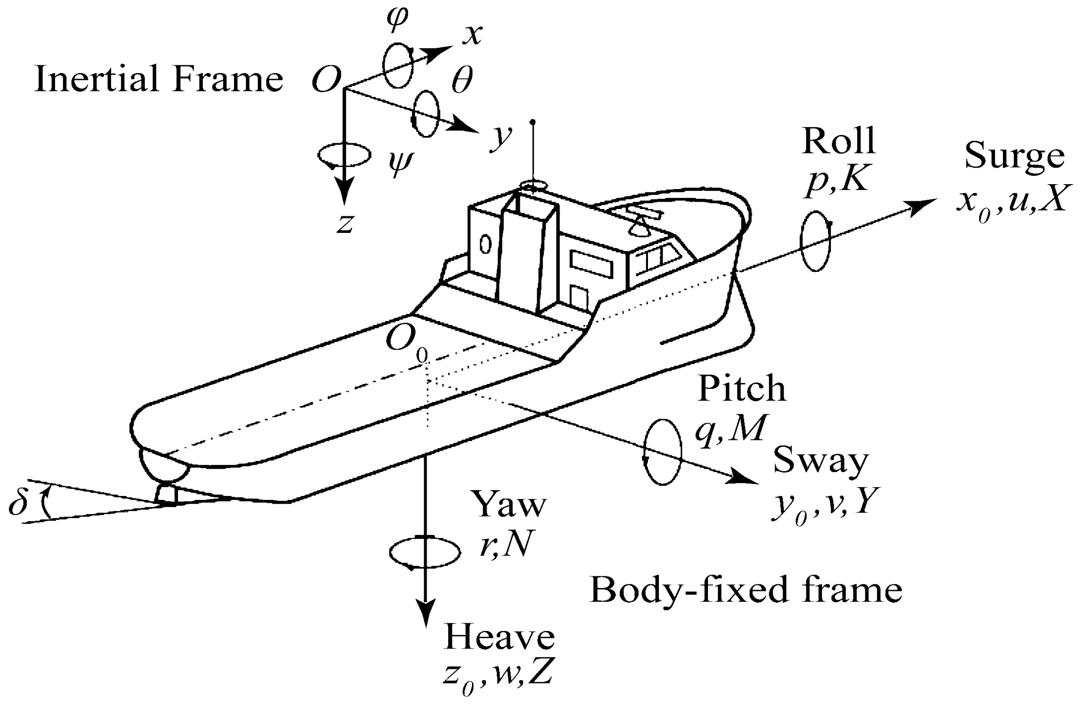
2.1. Ship Motion Model
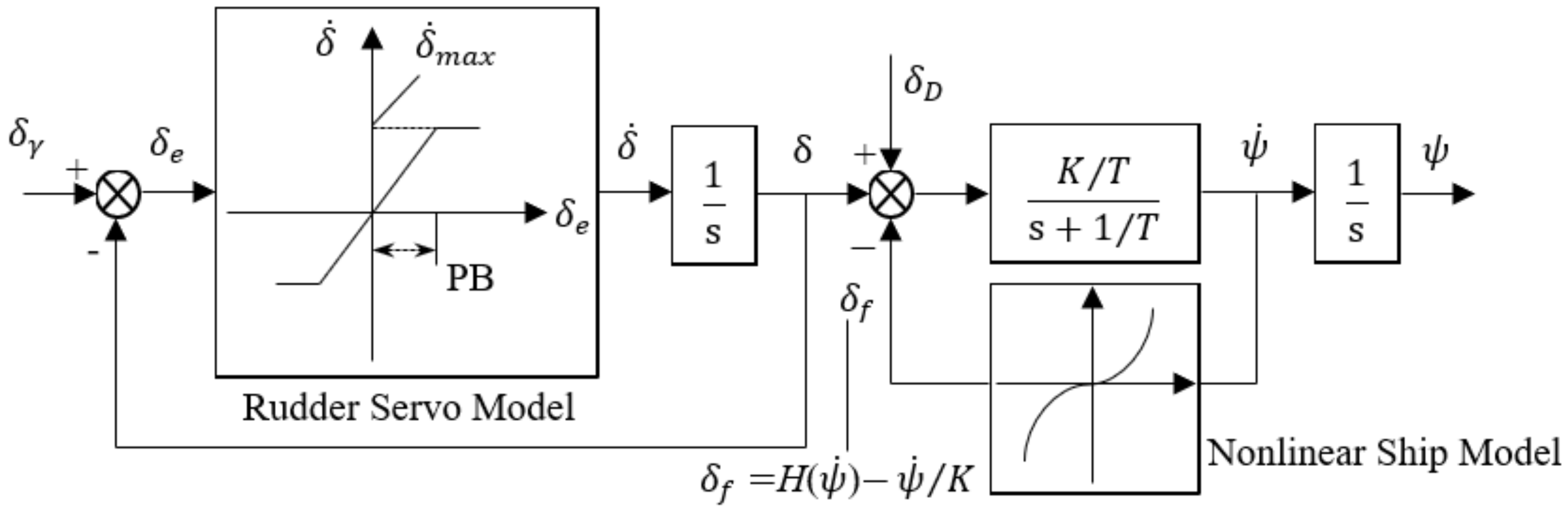
2.2. Nonlinear Ship Model
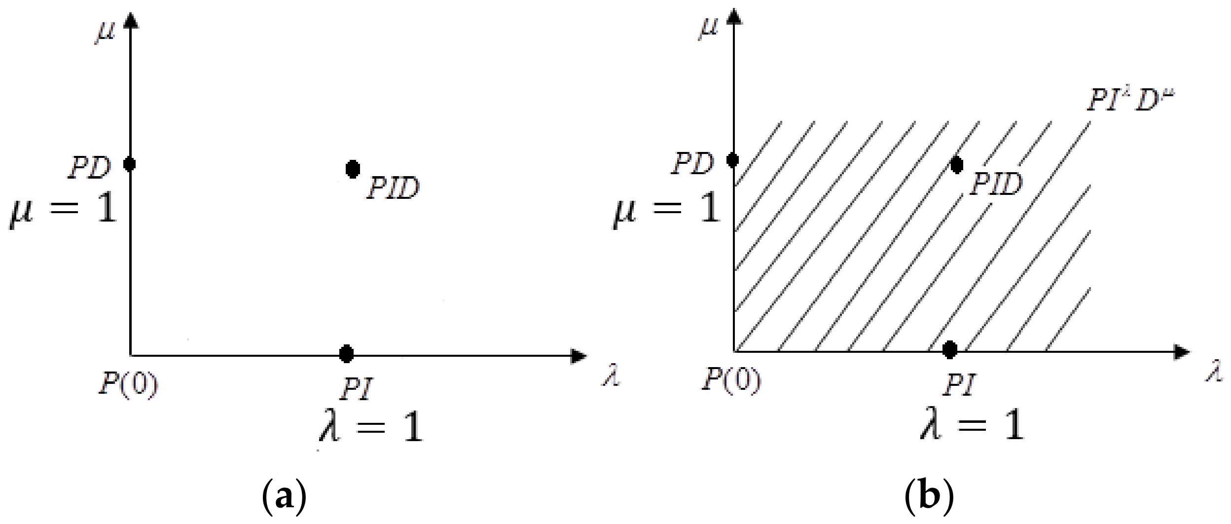
3. FO PIλDµ Controller
4. The FO PIλDµ Controller of a Ship’s Course
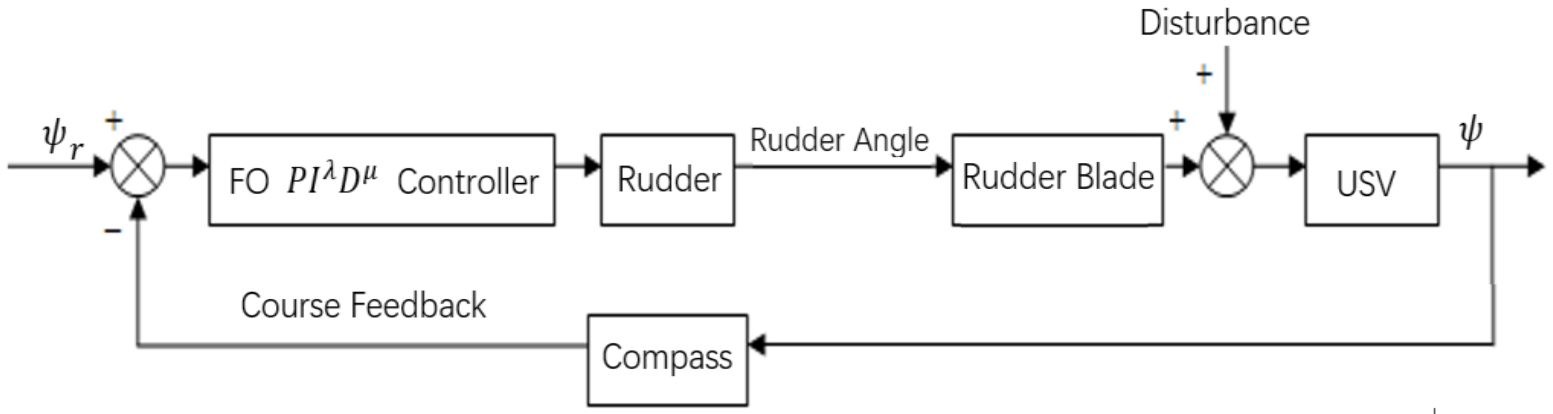
4.1. FO PIλDµ Controller Design
4.2. Autotuning of the FO PIλDµ Controller Based on the IPSO Algorithm
- If c1 and c2 are both set to 0, the particle flight velocity will remain constant, making it impossible to search the entire space;
- If c1 = 0, the particle loses its cognitive ability and easily falls into a local optimum solution;
- If c2 = 0, which leads to a lack of communication and cooperation between particles, the algorithm will fall into a local minimum, and the probability of obtaining an optimal solution will become smaller;
- Smaller values for both c1 and c2 result in particles flying away from the target area and oscillating in that area;
- With larger values for both c1 and c2, particles fly faster toward the target area, and this may also cause particles to fly away from the target area.
5. Simulations
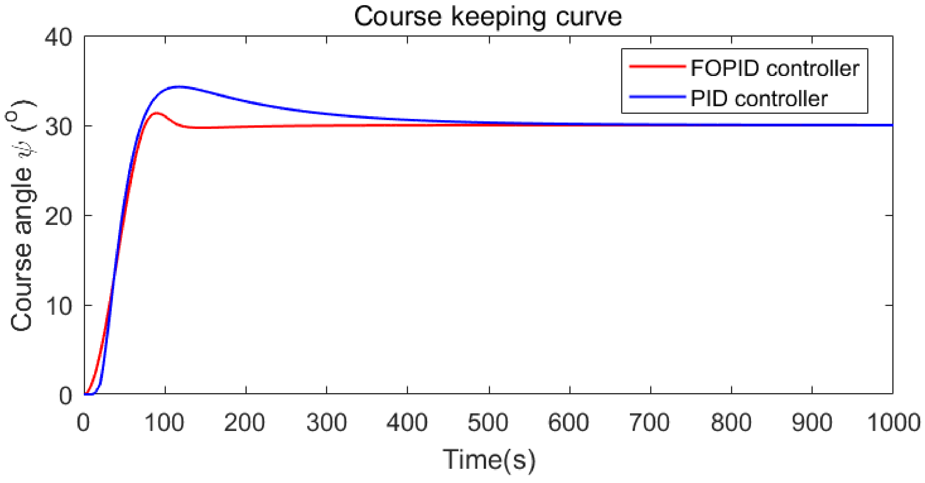
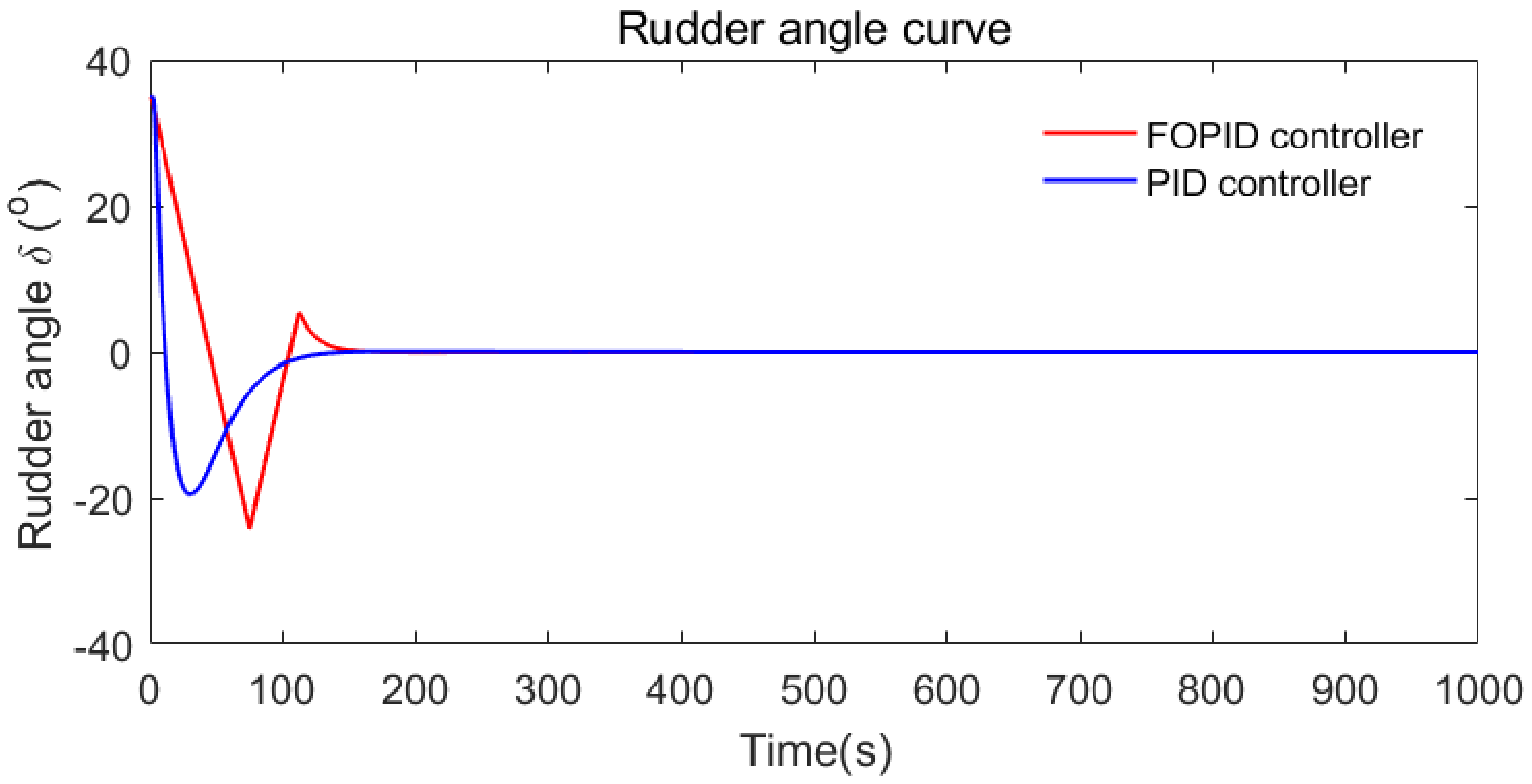
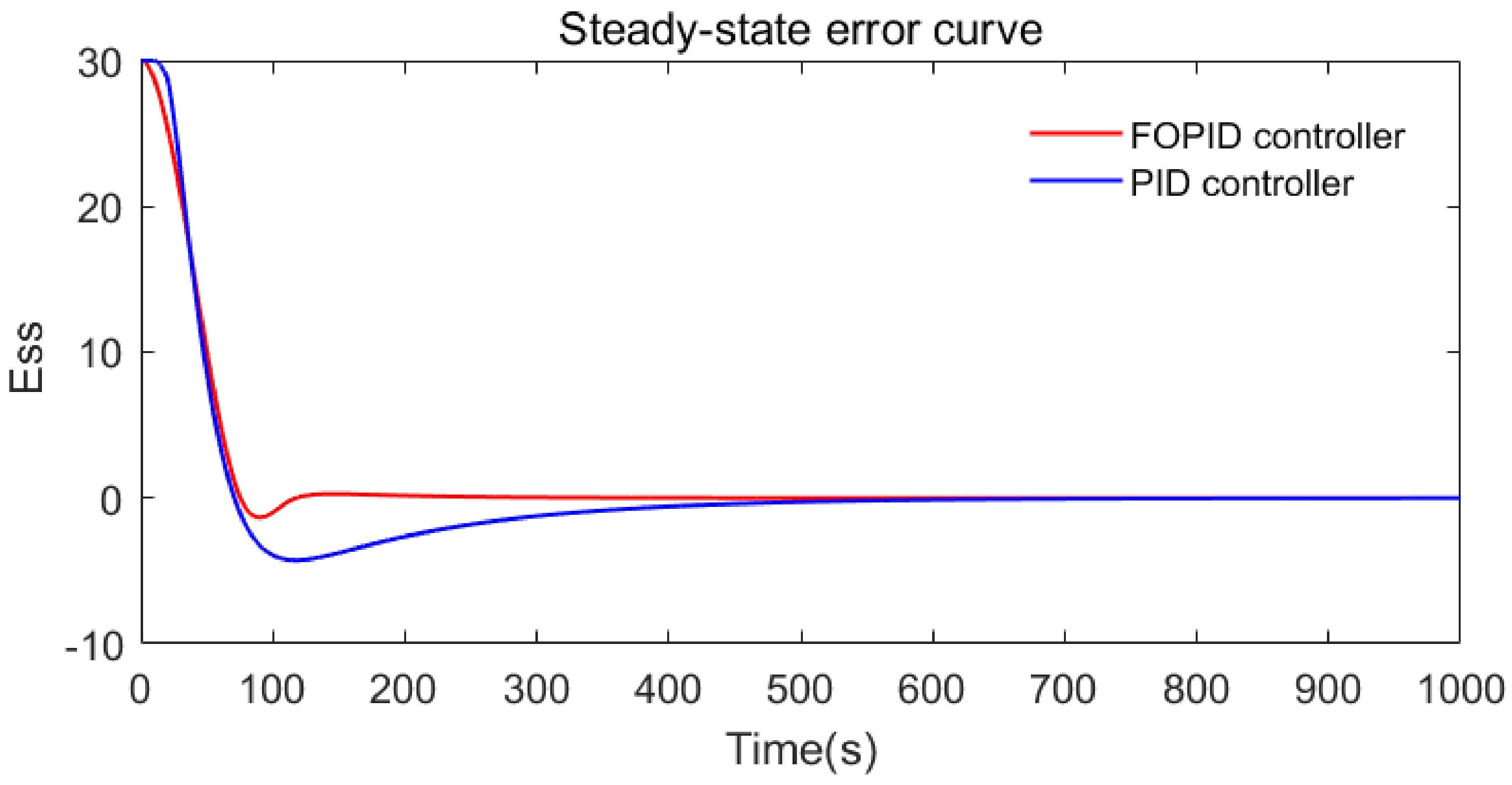
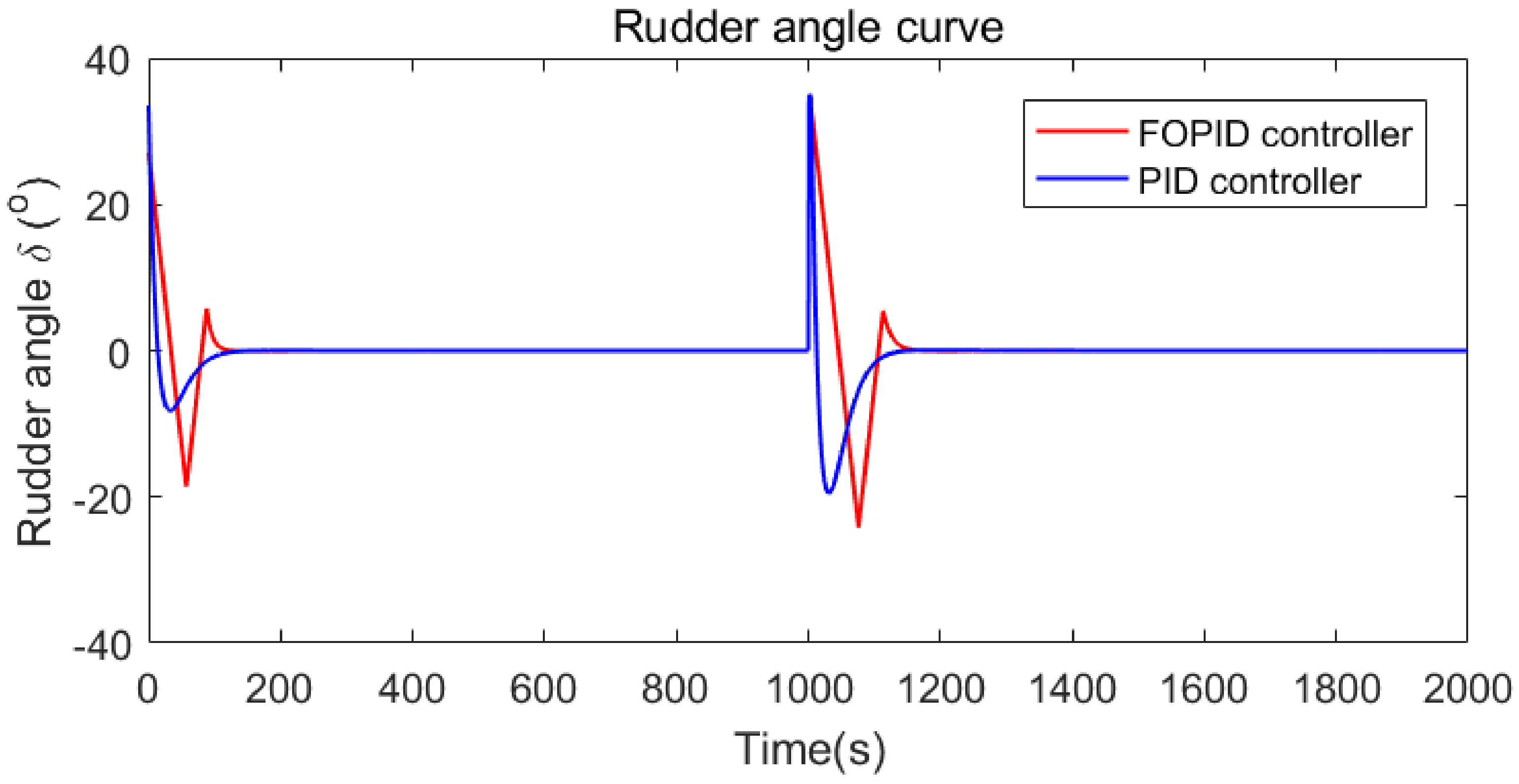
5.1. FO Controller
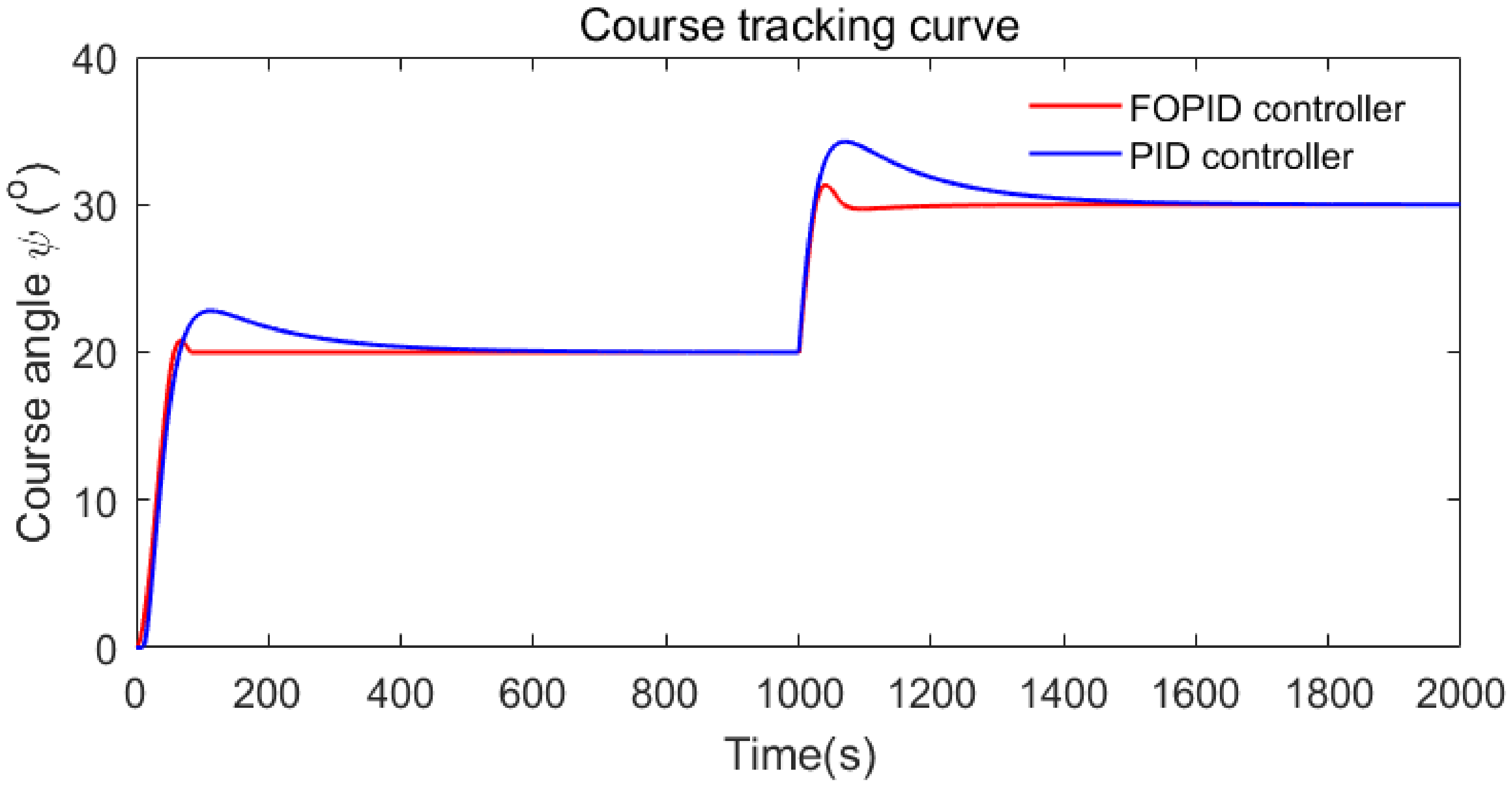
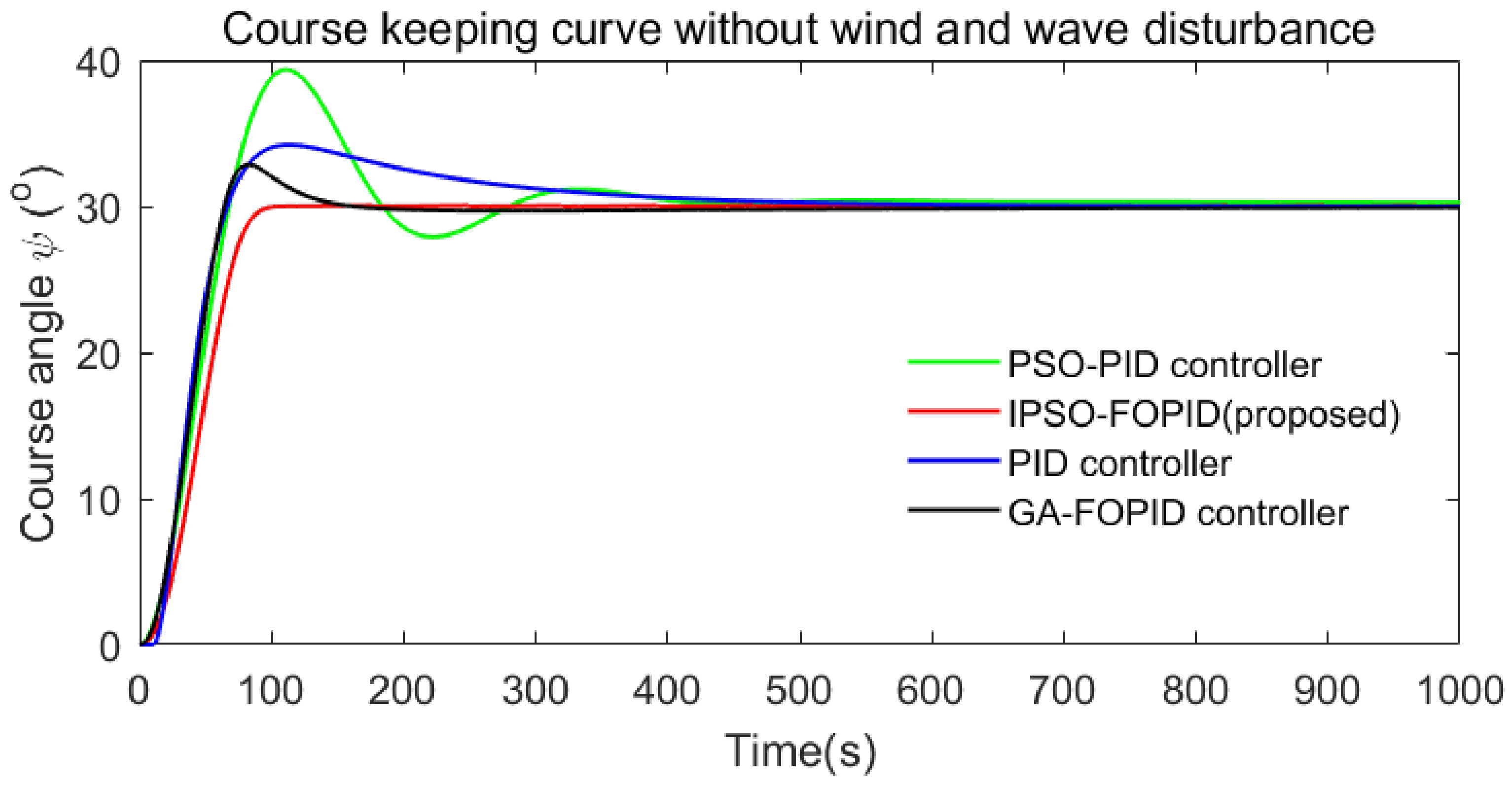
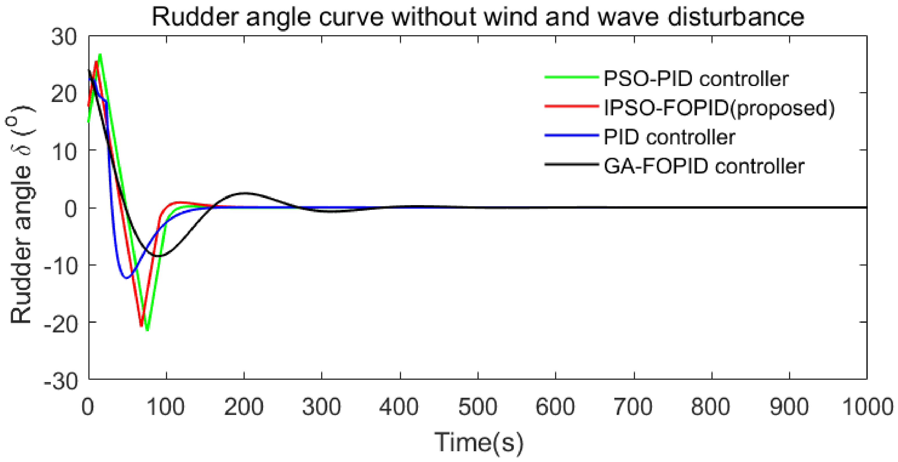
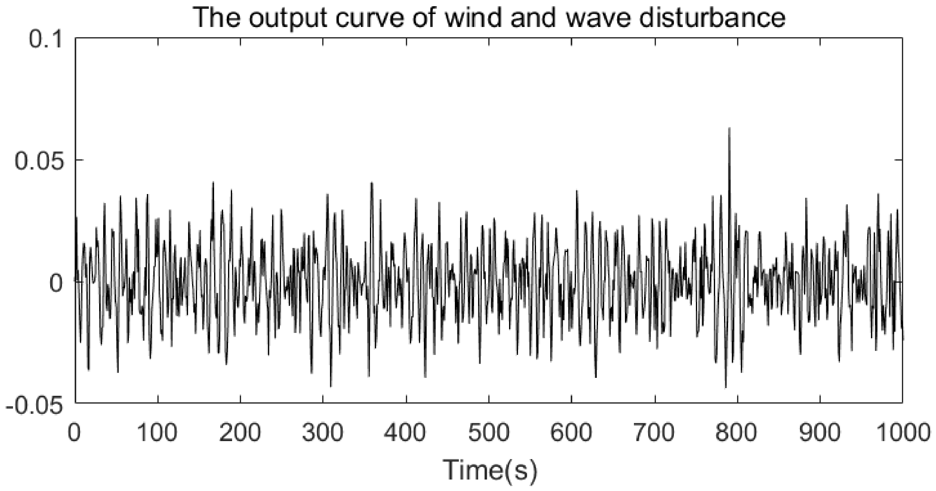
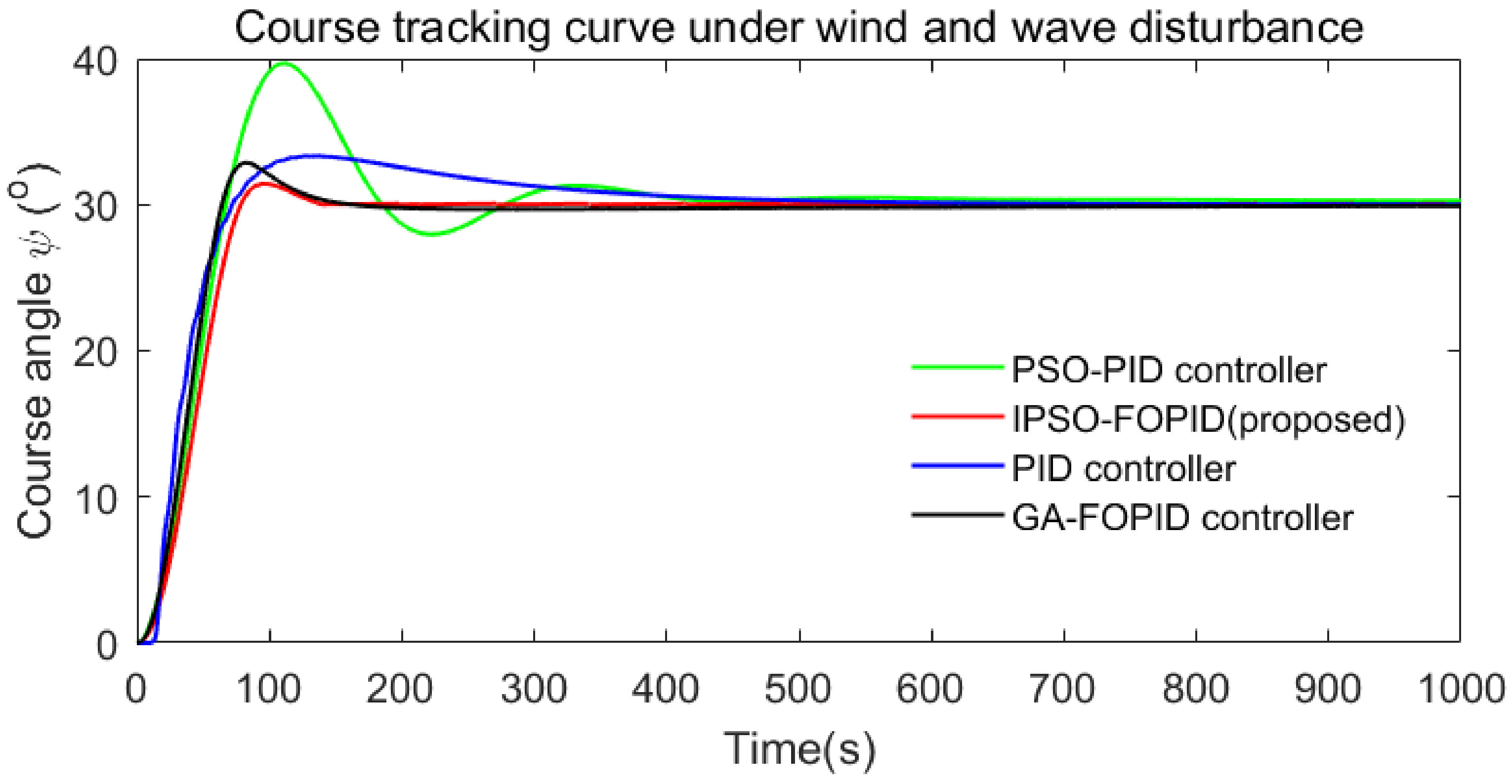
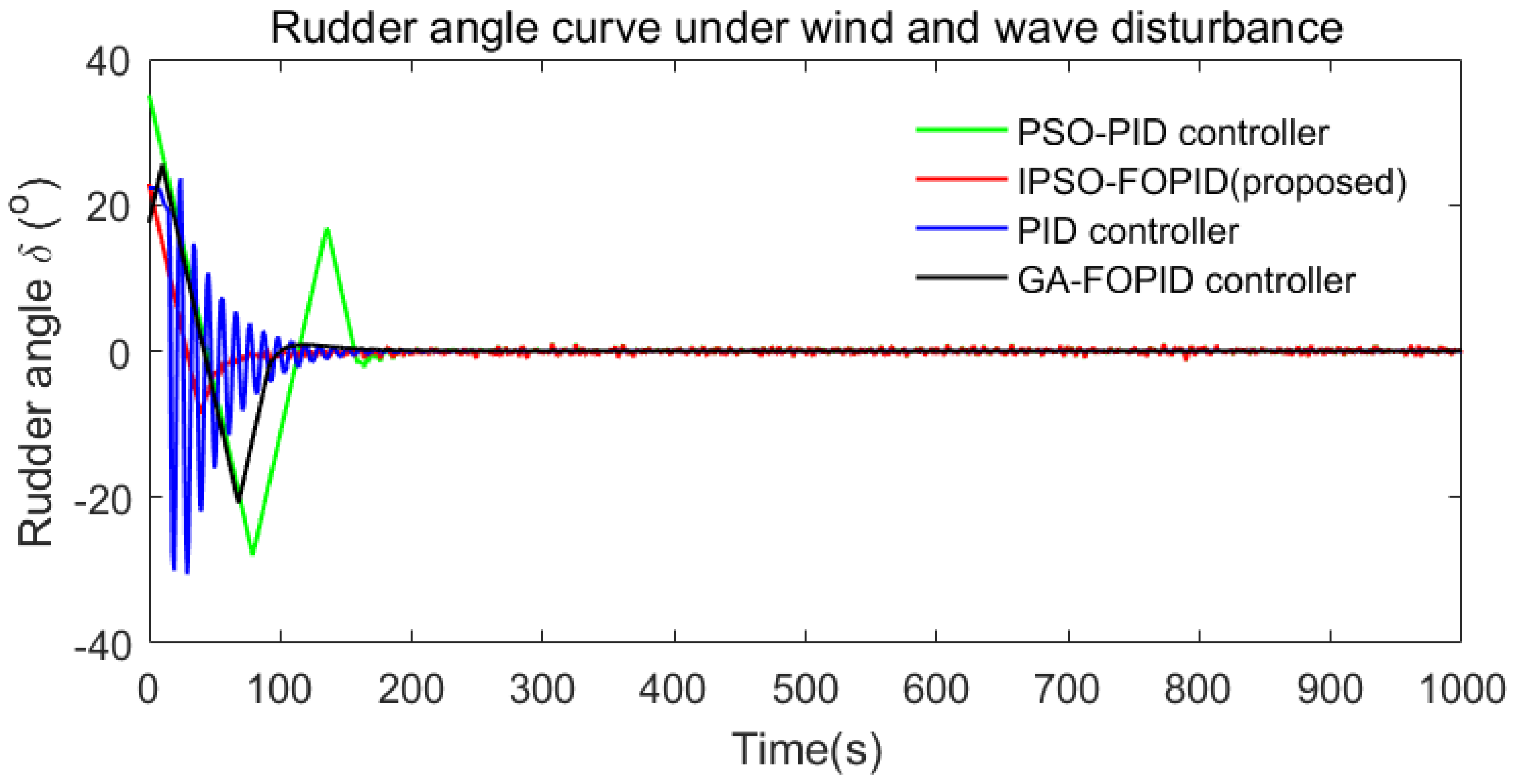
5.2. FO PIλDµ Controller Based on the IPSO Algorithm
6. Conclusions
Author Contributions
Funding
Institutional Review Board Statement
Informed Consent Statement
Data Availability Statement
Conflicts of Interest
References
- Park, B.S.; Kwon, J.W.; Kim, H. Neural network-based output feedback control for reference tracking of underactuated surface vessels. Automatica 2017, 77, 353–359. [Google Scholar] [CrossRef]
- Lu, Y.; Zhang, G.; Sun, Z.; Zhang, W. Robust adaptive formation control of underactuated autonomous surface vessels based on MLP and DOB. Nonlinear Dyn. 2018, 94, 503–519. [Google Scholar] [CrossRef]
- Liu, C.; Negenborn, R.R.; Chu, X.; Zheng, H. Predictive path following based on adaptive line-of-sight for underactuated autonomous surface vessels. J. Mar. Sci. Technol. 2018, 23, 483–494. [Google Scholar] [CrossRef]
- Sahu, B.K.; Subudhi, B.; Gupta, M.M. Stability Analysis of an Underactuated Autonomous Underwater Vehicle Using Extended-Routh’s Stability Method. Int. J. Autom. Comput. 2018, 15, 299–309. [Google Scholar] [CrossRef]
- Xie, W.; Reis, J.; Cabecinhas, D.; Silvestre, C. Design and experimental validation of a nonlinear controller for underactuated surface vessels. Nonlinear Dyn. 2020, 102, 2563–2581. [Google Scholar] [CrossRef]
- Kolmanovsky, I.; McClamroch, N.H. Developments in nonholonomic control problems. IEEE Control Syst. Mag. 1995, 15, 20–36. [Google Scholar]
- Le, M.D.; Nguyen, S.H.; Nguyen, L.A. Study on a new and effective fuzzy PID ship autopilot. Artif. Life Robot. 2004, 8, 197–201. [Google Scholar] [CrossRef]
- Gao, C.; Guo, J. On the existence of an optimal control of ship automatic steering instruments. J. Ocean Univ. China 2005, 4, 185–188. [Google Scholar] [CrossRef]
- Dlabač, T.; Ćalasan, M.; Krčum, M.; Marvučić, N. PSO-BASED PID controller design for ship course-keeping autopilot. Brodogradnja 2019, 70, 1–15. [Google Scholar] [CrossRef]
- Liu, S.; Fang, L. Application of H∞ control in rudder/flap vector robust control of a ship’s course. J. Mar. Sci. Appl. 2007, 6, 62–67. [Google Scholar] [CrossRef]
- Zhang, Q.; Zhang, M.; Hu, Y.; Zhu, G. Error-driven-based adaptive nonlinear feedback control of course-keeping for ships. J. Mar. Sci. Technol. 2021, 26, 357–367. [Google Scholar] [CrossRef]
- Wu, J.; Zeng, C.; Hu, Y. Indirect Adaptive Robust Control Design for Course Tracking of Ships Subject to Unknown Control Coefficient and Disturbances. Int. J. Control Autom. Syst. 2021, 19, 2059–2067. [Google Scholar] [CrossRef]
- Oldham, K.B.; Spanier, J. The Fractional Calculus; Academic Press: New York, NY, USA, 1974. [Google Scholar]
- Miller, K.S.; Ross, B. An Introduction to the Fractional Calculus and Fractional Differential Equations; Wiley: New York, NY, USA, 1993. [Google Scholar]
- Podlubny, I. Fractional Differential Equations; Academic Press: San Diego, CA, USA, 1999. [Google Scholar]
- Podlubny, I. Fractional-order System and Fractional-order Control. IEEE Trans. Autom. Control 1999, 44, 208–214. [Google Scholar] [CrossRef]
- Podlubny, I. Realization of Fractional-Order Control. Acta Montan. Slovaca 2003, 8, 233–235. [Google Scholar]
- Podlubny, I.; Petráš, I.; Vinagre, B.M. Analogue Realizations of Fractional-Order Controllers. Nonlinear Dyn. 2002, 29, 281–296. [Google Scholar] [CrossRef]
- Bingül, Z.A.F.E.R.; Karahan, O.Ğ.U.Z.H.A.N. Fractional PID controllers tuned by evolutionary algorithms for robot trajectory control. Turk. J. Electr. Eng. Comput. Sci. 2012, 20, 1123–1136. [Google Scholar]
- Zhang, C.; Tan, N.; Zhou, T.; Liu, M.; Shan, H. Research on Optimal Control of Subway Train Based on Fractional Order PID Controller. J. China Railw. Soc. 2018, 40, 8–14. [Google Scholar]
- Qi, Z.D.; Bian, H.J.; Leng, B.Y.; Shan, L. Design of a new fractional order PIλ–PDµ controller based on SQP. Control Decis. 2016, 31, 2275–2279. [Google Scholar]
- Safikhani Mohammadzadeh, H.; Tabatabaei, M. Design of Non-overshooting Fractional-Order PD and PID Controllers for Special Case of Fractional-Order Plants. J. Control Autom. Electr. Syst. 2019, 30, 611–621. [Google Scholar] [CrossRef]
- Kumar, J.; Kumar, V.; Rana, K.P.S. Fractional-order self-tuned fuzzy PID controller for three-link robotic manipulator system. Neural Comput. Appl. 2020, 32, 7235–7257. [Google Scholar] [CrossRef]
- Nasir, A.; Rasool, I.; Sibtain, D.; Kamran, R. Adaptive Fractional Order PID Controller Based MPPT for PV Connected Grid System under Changing Weather Conditions. J. Electr. Eng. Technol. 2021, 16, 2599–2610. [Google Scholar] [CrossRef]
- Izci, D.; Ekinci, S.; Eker, E.; Kayri, M. A novel modified opposition-based hunger games search algorithm to design fractional order proportional-integral-derivative controller for magnetic ball suspension system. Adv. Control Appl. Eng. Ind. Syst. 2022, 4, e96. [Google Scholar] [CrossRef]
- Altbawi, S.M.A.; Mokhtar, A.S.B.; Jumani, T.A. Optimal design of Fractional order PID controller based Automatic voltage regulator system using gradient-based optimization algorithm. J. King Saud Univ. Eng. Sci. 2021, in press. [Google Scholar] [CrossRef]
- Izci, D.; Ekinci, S.; Hekimoğlu, B. Fractional-Order PID Controller Design for Buck Converter System via Hybrid Lévy Flight Distribution and Simulated Annealing Algorithm. Arab. J. Sci. Eng. 2022, in press. [Google Scholar] [CrossRef]
- Cui, H.; Guan, Y.; Chen, H. Rolling element fault diagnosis based on VMD and sensitivity MCKD. IEEE Access 2021, 9, 120297–120308. [Google Scholar] [CrossRef]
- Deng, W.; Xu, J.; Gao, X.; Zhao, H. An enhanced MSIQDE algorithm with novel multiple strategies for global optimization problems. IEEE Trans. Syst. Man. Cybern. Syst. 2022, 52, 578–1587. [Google Scholar] [CrossRef]
- Ran, X.; Zhou, X.; Lei, M.; Tepsan, W.; Deng, W. A novel k-means clustering algorithm with a noise algorithm for capturing urban hotspots. Appl. Sci. 2021, 11, 11202. [Google Scholar] [CrossRef]
- Deng, W.; Zhang, X.X.; Zhou, Y.Q.; Liu, Y.; Zhou, X.B.; Chen, H.L.; Zhao, H.M. An enhanced fast non-dominated solution sorting genetic algorithm for multi-objective problems. Inform. Sci. 2022, 585, 441–453. [Google Scholar] [CrossRef]
- Li, T.Y.; Qian, Z.J.; Deng, W.; Zhang, D.Z.; Lu, H.H.; Wang, S.H. Forecasting crude oil prices based on variational mode decomposition and random sparse Bayesian learning. Appl. Soft Comput. 2021, 113, 108032. [Google Scholar] [CrossRef]
- Shao, H.D.; Lin, J.; Zhang, L.W.; Galar, D.; Kumar, U. A novel approach of multisensory fusion to collaborative fault diagnosis in maintenance. Inf. Fusion 2021, 74, 65–76. [Google Scholar] [CrossRef]
- Deng, W.; Xu, J.; Zhao, H.; Song, Y. A novel gate resource allocation method using improved PSO-based QEA. IEEE Tran. Intell. Transp. Syst. 2022, 23, 1737–1745. [Google Scholar] [CrossRef]
- Wu, X.H. Ship Maneuverability and Seakeeping; China Communications Press: Beijing, China, 1999. [Google Scholar]
- Wei, M.; Guo, C.; Liu, Y. Robust Adaptive path following for underactuated surface vessels with uncertain dynamics. J. Mar. Sci. 2012, 11, 244–250. [Google Scholar]
- Fossen, T.I. Guidance and Control of Ocean Vehicle; John Wiley & Sons Ltd.: Chichester, UK, 1994. [Google Scholar]
- Oustaloup, A.; Levron, F.; Mathieu, B.; Nanot, F.M. Frequency-band complex non-integer differentiator: Characterization and synthesis. IEEE Trans. Circuits Syst.-I Fundam. Theory Appl. 2000, 47, 25–39. [Google Scholar] [CrossRef]
- Xue, D.Y.; Zhao, C.N. Fractional order PID controller design for fractional order system. Control Theory Appl. 2007, 24, 771–776. [Google Scholar]
- Li, T.Y.; Shi, J.Y.; Zhang, D.Z. Color image encryption based on joint permutation and diffusion. J. Electron. Imaging 2021, 30, 013008. [Google Scholar] [CrossRef]
- Zhang, Z.H.; Min, F.; Chen, G.S.; Shen, S.P.; Wen, Z.C.; Zhou, X.B. Tri-partition state alphabet-based sequential pattern for multivariate time series. Cogn. Comput. 2021, 1–19. [Google Scholar] [CrossRef]
- Chen, H.; Zhang, Q.; Luo, J. An enhanced Bacterial Foraging Optimization and its application for training kernel extreme learning machine. Appl. Soft Comput. 2020, 86, 105884. [Google Scholar] [CrossRef]
- Deng, W.; Shang, S.; Cai, X.; Zhao, H.; Zhou, Y.; Chen, H.; Deng, W. Quantum differential evolution with cooperative coevolution framework and hybrid mutation strategy for large scale optimization. Knowl.-Based Syst. 2021, 224, 107080. [Google Scholar] [CrossRef]
- Wang, X.; Wang, H.Y.; Du, C.Z.; Fan, X.; Cui, L.; Chen, H.; Deng, F.; Tong, Q.; He, M.; Yang, M.; et al. Custom-molded offloading footwear effectively prevents recurrence and amputation, and lowers mortality rates in high-risk diabetic foot patients: A multicenter, prospective observational study. Diabetes Metab. Syndr. Obes. Targets Ther. 2022, 15, 103–109. [Google Scholar]
- Wei, Y.Y.; Zhou, Y.Q.; Luo, Q.F.; Deng, W. Optimal reactive power dispatch using an improved slime mould algorithm. Energy Rep. 2021, 7, 8742–8759. [Google Scholar] [CrossRef]
- Wang, L.Z.; Zhang, J.B.; Liu, P.; Choo, K.K.; Huang, F. Spectral-spatial multi-feature-based deep learning for hyperspectral remote sensing image classification. Appl. Soft Comput. 2017, 21, 213–221. [Google Scholar] [CrossRef]
- Luo, X.; Shen, Z.; Xue, R. Unsupervised band selection method based on importance-assisted column subset selection. IEEE Access 2018, 7, 517–527. [Google Scholar] [CrossRef]
- Chang, C.I.; Kuo, Y.M.; Chen, S. Self-mutual information-based band selection for hyperspectral image classification. IEEE Trans. Geosci. Remote Sens. 2021, 59, 5979–5997. [Google Scholar] [CrossRef]
- Lin, Z.; Yan, L. A support vector machine classifier based on a new kernel function model for hyperspectral data. Mapp. Sci. Remote Sens. 2015, 53, 85–101. [Google Scholar] [CrossRef]
- He, Z.Y.; Shao, H.D.; Zhong, X.; Zhao, X.Z. Ensemble transfer CNNs driven by multi-channel signals for fault diagnosis of rotating machinery cross working conditions. Knowl.-Based Syst. 2020, 207, 106396. [Google Scholar] [CrossRef]
- Li, T.Y.; Shi, J.Y.; Deng, W.; Hu, Z.D. Pyramid particle swarm optimization with novel strategies of competition and cooperation. Appl. Soft Comput. 2021, 121, 108731. [Google Scholar]
- Deng, W.; Li, Z.; Li, X.; Chen, H.; Zhao, H. Compound fault diagnosis using optimized MCKD and sparse representation for rolling bearings. IEEE Trans. Instrum. Meas. 2022, in press. [Google Scholar] [CrossRef]
- Izci, D. A novel improved atom search optimization algorithm for designing power system stabilizer. Evol. Intell. 2021, in press. [Google Scholar] [CrossRef]
- Izci, D. Design and application of an optimally tuned PID controller for DC motor speed regulation via a novel hybrid Lévy flight distribution and Nelder–Mead algorithm. Trans. Inst. Meas. Control 2021, 43, 3195–3211. [Google Scholar] [CrossRef]
- Eberhart, R.C.; Kennedy, J. A New Optimizer Using Particle Swarm Theory. In Proceedings of the 6th International on Symposium of Micromachine Human Science, Nagoya, Japan, 4–6 October 1995; pp. 39–43. [Google Scholar]
- Kennedy, J.; Eberhart, R.C. Particle swarm optimization. In Proceedings of the IEEE International Conference on Neural Networks, Perth, Australia, 27 November–1 December 1995; pp. 1942–1948. [Google Scholar]
- Angeline, P.J. Using selection to improve particle swarm optimization. In Proceedings of the IEEE International Conference on Evolutionary Computation and IEEE World Congress on Computational Intelligence, Anchorage, AK, USA, 4–9 May 1998; pp. 84–89. [Google Scholar]
- Naka, S.; Genji, T.; Yura, T.; Fukuyama, Y. A hybrid particle swarm optimization for distribution state estimation. IEEE Trans. Power Syst. 2003, 18, 60–68. [Google Scholar] [CrossRef]
- Wonohadidjojo, D.M.; Kothapalli, G.; Hassan, M.Y. Position control of electro-hydraulic actuator system using fuzzy logic controller optimized by particle swarm optimization. Int. J. Autom. Comput. 2013, 10, 181–193. [Google Scholar] [CrossRef] [Green Version]
- Jia, X.L.; Zhang, X.K. Intelligent Control of Ship Motion with H∞ Robust Control; Dalian Maritime University Press: Dalian, China, 2002. [Google Scholar]


| Algorithm | Particles m | Weight ω | Learning Factors c1, c2 | Maximum Speed Vmax | Maximum Iterations Tmax |
|---|---|---|---|---|---|
| PSO | 20 | 1 | 2, 2 | 1 | 100 |
| IPSO | 20 | 1 | Equations (30) and (31) | 1 | 100 |
| Structure | Value | Structure | Value |
|---|---|---|---|
| length of ship | 280 m | length of two columns | 267 m |
| width of ship | 39.8 m | distance of gravity center | 2.64 m |
| area of Rudder | 61.0 m2 | square coefficient | 0.67 |
| no-load weight | 3.5453 M tons | full load weight | 6.5531 M tons |
| draft | 12.532 m | draft with fully load | 14.023 m |
| Controller Type | Adjust Time ts | Rise Time tr | Overshoot M | Ess |
|---|---|---|---|---|
| FO PIλDµ | 114 | 75 | 4.42% | 0.002 |
| PID controller | 519 | 71 | 14.25% | 0.007 |
| V (knots) | K | T | α | β |
|---|---|---|---|---|
| 27.1 | 0.2676 | 186.9556 | 10.4915 | 7.5343 |
| 26.5 | 0.2617 | 191.1885 | 10.7291 | 8.0578 |
| 24.5 | 0.2419 | 206.7958 | 11.6049 | 10.1966 |
| 22.5 | 0.2222 | 225.1776 | 12.6366 | 13.1644 |
| 19.8 | 0.1955 | 255.8837 | 14.3601 | 19.3172 |
| Controller Type | Adjust Time ts | Rise Time tr | Overshoot M | Ess |
|---|---|---|---|---|
| IPSO-FOPID (proposed) | 103 | 103 | 0.03% | 0.005 |
| PSO-PID | 416 | 67 | 31.16% | 0.024 |
| PID | 519 | 71 | 14.25% | 0.007 |
| GA-FOPID | 163 | 65 | 9.53% | 0.086 |
Publisher’s Note: MDPI stays neutral with regard to jurisdictional claims in published maps and institutional affiliations. |
© 2022 by the authors. Licensee MDPI, Basel, Switzerland. This article is an open access article distributed under the terms and conditions of the Creative Commons Attribution (CC BY) license (https://creativecommons.org/licenses/by/4.0/).
Share and Cite
Li, G.; Li, Y.; Chen, H.; Deng, W. Fractional-Order Controller for Course-Keeping of Underactuated Surface Vessels Based on Frequency Domain Specification and Improved Particle Swarm Optimization Algorithm. Appl. Sci. 2022, 12, 3139. https://doi.org/10.3390/app12063139
Li G, Li Y, Chen H, Deng W. Fractional-Order Controller for Course-Keeping of Underactuated Surface Vessels Based on Frequency Domain Specification and Improved Particle Swarm Optimization Algorithm. Applied Sciences. 2022; 12(6):3139. https://doi.org/10.3390/app12063139
Chicago/Turabian StyleLi, Guangyu, Yanxin Li, Huayue Chen, and Wu Deng. 2022. "Fractional-Order Controller for Course-Keeping of Underactuated Surface Vessels Based on Frequency Domain Specification and Improved Particle Swarm Optimization Algorithm" Applied Sciences 12, no. 6: 3139. https://doi.org/10.3390/app12063139