Review

NMR in Metabolomics: From Conventional Statistics to Machine Learning and Neural Network Approaches

1
Department of Mathematical and Computational Science, Physical Science and Earth Science, University of Messina, Viale F. Stagno D’Alcontres 31, I-98166 Messina, Italy
2
Department of Chemical, Biological, Pharmaceutical and Environmental Sciences, University of Messina, Viale F. Stagno D’Alcontres 31, I-98166 Messina, Italy
*
Author to whom correspondence should be addressed.
Appl. Sci. 2022, 12(6), 2824; https://doi.org/10.3390/app12062824
Submission received: 31 January 2022 / Revised: 26 February 2022 / Accepted: 1 March 2022 / Published: 9 March 2022

Abstract

:
NMR measurements combined with chemometrics allow achieving a great amount of information for the identification of potential biomarkers responsible for a precise metabolic pathway. These kinds of data are useful in different fields, ranging from food to biomedical fields, including health science. The investigation of the whole set of metabolites in a sample, representing its fingerprint in the considered condition, is known as metabolomics and may take advantage of different statistical tools. The new frontier is to adopt self-learning techniques to enhance clustering or classification actions that can improve the predictive power over large amounts of data. Although machine learning is already employed in metabolomics, deep learning and artificial neural networks approaches were only recently successfully applied. In this work, we give an overview of the statistical approaches underlying the wide range of opportunities that machine learning and neural networks allow to perform with accurate metabolites assignment and quantification.Various actual challenges are discussed, such as proper metabolomics, deep learning architectures and model accuracy.

1. Introduction

Metabolomics corresponds to the part of omics sciences that investigates the whole set of small molecule metabolites in an organism, representing a large number of compounds, such as a portion of organic acids, amino acids, carbohydrates, lipids, etc. [1,2,3]. The investigation and the recording of metabolites by target analysis, metabolic profiling and metabolic fingerprinting (i.e., extracellular metabolites) are fundamental steps for the discovery of biomarkers, helping in diagnoses and designing appropriate approaches for drug treatment of diseases [4,5]. There are many databases available with metabolomics data, including spectra acquired by nuclear magnetic resonance (NMR) and mass spectrometry (MS), but also metabolic pathways. Among them, we mention the Human Metabolome Database (HMDB) [6] and Biological Magnetic Resonance Bank (BMRB) [7] that contain information on a large number of metabolites gathered from different sources. By means of the corresponding web platform, it is possible, for instance, to search for mono- and bi-dimensional spectra of metabolites, starting from their peak position [3]. However, metabolomics databases still lack homogeneity mainly due to the different acquisition conditions, including employed instruments. Thus, the definition of uniform and minimum reporting standards and data formats would allow an easier comparison and a more accurate investigation of metabolomics data [8].
In recent years, NMR has become one of the most employed analytical non-destructive techniques for clinical metabolomics studies. In fact, it allows to detect and quantify metabolic components of a biological matrix whose concentration is comparable or bigger than 1 μ M (see Appendix A). Such sensitivity, relatively low if compared with other MS techniques, allows to assign up to 20 metabolites in vivo, and up to 100 metabolites in vitro [9,10,11]. Numerous strategies are being designed to overcome actual limitations, including a lower selectivity compared to the MS technique coupled with gas or liquid chromatography (GC-MS and LC-MS, respectively) and a low resolution for complex biological matrices. These include the development of new pulse sequences mainly involving field gradients for observing multidimensional hetero- or homo-nuclear correlations [12]. Within metabolomics investigations, NMR analyses are usually coupled with statistical approaches: sample randomization allows to reduce the correlation between confounding variables, sample investigation order and experimental procedures. In the last ten years, nested stratified proportional randomization and matched case-control design were adopted in the case of imbalanced results [13,14,15].
In any case, data pre-processing is a relevant step before performing data analysis by means of a conventional approach or a statistical one. The goal of pre-processing is to homogenize the acquired data, avoiding the presence of instrumental bias mainly involving peaks’ features for a better quantification of metabolites. For example, the pre-processing of NMR spectra concerns phasing, baseline correction, peak alignment, apodization procedures, normalization and binning [16,17] (see Figure 1). In particular, the binning procedure corresponding to the spectral segmentation is performed mainly in those cases of challenging spectral alignment or simply for reducing the data points [18]. Even though binning reduces data resolution, binning procedures are commonly used [19,20,21].
For what concerns normalization, recorded spectra are usually normalized by the total integrated area and thus the metabolites concentration can be compared among different samples. In the case of large signals variation, probabilistic quotient normalization can be adopted instead [24]. Finally, deconvolution is also employed for the necessary assignment and quantification of those metabolites whose signals overlap [25,26]. All these pre-processing methods are also chosen, taking into account that the approaches adopted for the data processing are essentially dual: (1) chemometrics, consisting in the employment of statistical analysis for the recognition of similar patterns and for the significant determination of intensity values, and (2) quantitative metabolomics, based on an initial assignment and quantification of metabolites with the subsequent statistics. We outline that, from one side, chemometrics allows an automatic and non-biased classification of metabolites, whereas from the other side, it needs a big number of uniform spectra. These requirements do not apply for quantitative metabolomics [27,28].
In order to gain useful insights and a corresponding interpretation of NMR outcomes, it is indeed mandatory to use statistical and bioinformatic tools, considering the complex output generated [22]. In this work, we discuss the main statistical approaches currently used for NMR-based metabolomics analysis, pointing out the advantages and disadvantages. Illustrative examples are reported, and the actual challenges influencing the analysis are also discussed. On the basis of these evidences, it emerged that innovative experimental procedures would need to be implemented in order to improve the potentiality of existing approaches (i.e., adequate sample sizes and conditions), thereby combining their complementing features with the aim to achieve most of the metabolomic information from an NMR measurement. Nevertheless, on considering the high complexity of biological systems, each regulation level, including the genome, should be considered, yielding corresponding insights on cellular processes. Thus, data coming from different biological levels should be integrated within the same analysis for the observation of interconnectivity changes between the different cellular components. In this context, neural network-based approaches could be adequate in responding to this major challenge and indeed to the exploitation of proper approaches for the weighted consideration of data corresponding to different layers of biological organization.

2. Conventional Approaches

2.1. Unsupervised Methods

In the analysis of large metabolomic NMR datasets, unsupervised techniques are applied with the aim to identify any significant pattern within unlabeled databases without any human action. Below, we introduce and describe several unsupervised methods, highlighting their characteristics and implementation procedures. In particular, we describe the following unsupervised techniques: (a) principal component analysis (PCA); (b) clustering; (c) self-organizing maps (SOMs).

2.1.1. Principal Component Analysis (PCA)

Principal component analysis (PCA) is employed for lowering the dimensionality of high-dimensional datasets, preserving as much information as possible by means of a “linear” multivariate analysis [29,30]. This approach employs a linear transformation to define a new smaller set of “summary indices”—or “principal components” (PCs)—that are more easily visualized and analyzed [31]. In this frame, principal components correspond to new variables obtained by the linear combination of the initial variables by solving an eigenvalue/eigenvector problem. The first principal component (PC1) represents the “path” along which the variance of the data is maximized. As happens for the first principal component, the second one (PC2) also defines the maximum variance in the database. Nevertheless, it is completely uncorrelated to the PC1 following a direction that is orthogonal to the first component path. This step reiterates based on the dimensionality of the system, where a next principal component is the direction orthogonal to the prior components with the most variance. If there are significant distinctions between the ranges of initial variables (those variables with smaller ranges will be dominated by those with larger ones), distorted results may occur. To avoid this kind of problem, it is required to perform a standardization operation before executing PCA that corresponds to a transformation of the data into comparable scales. This can be done by using different scaling transformations, such as autoscaling, the generalized logarithm transform or the Pareto scaling with the aim to enhance the importance of small NMR signals, whose variation is more affected by the noise [32]. One of the most used transformation is the mean centered autoscaling:
v a l u e     m e a n s t . d e v i a t i o n ,
Furthermore, the computation of the covariance matrix is required to discard redundant information mainly due to the presence of any relationship between the initial variables of the data. The covariance matrix is symmetric (a n   ×   n ) being composed by the covariances of all pairs of the considered n variables x 1 , . . . , x n :
C o v x 1 , x 1 C o v x 1 , x n C o v x n , x 1 C o v x n , x n
In this frame, PCs can be obtained by finding the eigenvectors and eigenvalues from this covariance matrix. Figure 2 shows a graph with only three variables axes of the n-dimensional variables space. The red point in this figure represents the average point used to move the origin of the coordinate system by means of the mean-centering procedure in the standardization process. Once we define PC1 and PC2, as shown in Figure 2, they define a plane that allows inspecting the organization of the studied database. Further, the projection of the data with respect to the new variables (PCs) is called the score plot, and if the data are statistically different/similar, they can be regrouped and classified.
PCA is usually applied in NMR-metabolomic studies because it simplifies the investigation of hundreds of thousands of chemical components in metabolomic database composed of several collected NMR spectra. In this way, each NMR spectrum is confined to a single point in the score plot in which similar spectra are regrouped, and differences on the PC axes shed light on experimental variations between the measurements [28,33,34,35]. However, it is noteworthy that PCA, like the other latent structure techniques, must be applied to matrices where the number of cases is greater than the number of variables [36].
The PCA technique can also be combined with other statistical approaches, including the analysis of variance (ANOVA) as reported by Smilde et al. [37] in their ANOVA-simultaneous component analysis (ASCA). This method is able to associate observed data changes to the different experimental designs. It is applied to metabolomics data, for example, to study variations of the metabolites level in human saliva due to oral rinsing [38], or the metabolic responses of yeast at different starving conditions [39].

2.1.2. Clustering

Clustering is a data analysis technique used to regroup unlabeled data on the basis of their similarities or differences. Examples of clustering algorithms are essentially the following: exclusive, overlapping, hierarchical, and probabilistic clustering [40,41]. Exclusive and overlapping clustering can be described together because they differ for the existence of one or multiple data points in one or more clustered sets. In fact, while exclusive clustering establishes that a data point can occur only in one cluster, overlapping clustering enables data points to be part of multiple clusters with different degrees of membership. Exclusive and overlapping clustering are hard or k-means clustering and soft or fuzzy k-means clustering, respectively [42,43,44]. In hard clustering, every element in a database might be a part of a single and precise cluster, whereas in soft clustering, there is a probability of having each data point into a different cluster [44]. Generally speaking, k-means clustering is a “distance-based” method in which each “clustered set” is linked with a centroid that is considered to minimize the sum of the distances between data points in the cluster.
Hierarchical clustering analysis (HCA) is used to recognize non-linear evolution in the data—contrary to what was done by the PCA which shows a linear trend—by means of a regrouping of features sample by sample without having any previous information [45]. This clustering method could be divided in two groups: (i) agglomerative clustering, and (ii) divisive clustering [46,47]. The first one allows to keep data points separate at first, unifying them iteratively later until it one cluster with a precise similarity between the data points is obtained. In the opposite way, divisive clustering creates a separation of data points in a data cluster on the basis of their differences. The clustering analysis leads to dendrograms that are diagrams in which the horizontal row represents the linked residues, whereas the vertical axis describes the correlation between a residue and previous groups. Figure 3 reports a dendrogram obtained by means of hierarchical cluster analysis performed on 1 H NMR data on the plasma metabolome of 50 patients with early breast cancer [48]. This kind of analysis allowed to discriminate among three different groups: LR-1 (red), LR-2 (blue) and LR-3 (green). They are characterized by significantly different levels of some metabolites, such as lactate, pyruvate and glutamin [48]. Furthermore, covariance analysis of NMR chemical shift changes allows defining functional clusters of coupled residues [49].
Clustering has been largely applied for metabolomic studies covering fields from medicine to food science, as is reported in the Applications section (Section 4). Here, we anticipate that clustering is essentially adopted for samples’ classification by grouping metabolites without any external bias. This allows entering into the details of the precise metabolic pathways that may provide a connection between metabolomics and molecular biology. In such a way, many biomedical applications, including diagnostics and drug synthesis, would reach important improvements.

2.1.3. Self-Organizing Maps (SOMs)

Self-organizing maps (SOMs) were introduced by Kohonen [50] and are widely employed to cluster a database, reduce its dimension and detect its properties by projecting the original data in a new discrete organization of smaller dimensions. This is performed by weighting the data throughout proper vectors in order to achieve the best representation of the sample. Starting from a randomly selected vector, the algorithm constructs the map of weight vectors for defining the optimal weights, providing the best similarity to the chosen random vector. Vectors with weights close to the optimum are linked with each unit of the map allowing to categorize objects in map units. Then, the relative weight and the total amount of neighbors reduce over time. Therefore, SOMs have the great power of reducing the dimensionality of the system while preserving its topology. For that reason, they are commonly adopted for data clustering and as a visualization tool. Another great asset of SOMs concerns the shapes of the clusters that do not require being chosen before applying the algorithm, whereas other clustering techniques usually work well on specific cluster shapes [51]. However, some limitations are evidenced using SOMs. In fact, they are normally of low quality, and the algorithm must be run many times before a satisfactory outcome is reached. Further, it is not easy to furnish information about the whole data distribution by only observing the raw map. Figure 4 reports the cluster of subjects involved in the study of renal cell carcinoma (RCC) by (NMR)-based serum metabolomics that was generated by using SOM (including the weighted maps for the considered 16 metabolites) [52].
The achieved results clearly separate healthy subjects (left region) and RCC patients (right region) within the SOM. Moreover, the weighted maps of the individual metabolites allow to identify a biomarker cluster including the following seven metabolites: alanine, creatine, choline, isoleucine, lactate, leucine, and valine. These may be considered for an early diagnosis of renal cell carcinoma [52].

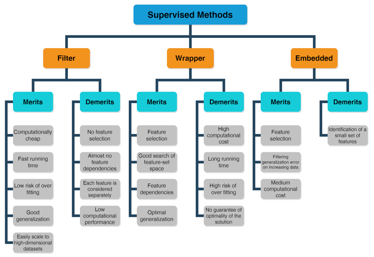
2.2. Supervised Methods

Problems or datasets having response variables (discrete or continuous) are generally treated with supervised methods. We distinguish between classification or regression problems, depending on whether the variables are discrete or continuous, respectively. The supervised technique is based on the association between the response variable (used to drive the model training) and the predictors (namely covariates) with the aim to perform precise predictions [53,54,55]. In fact, first, a training dataset is used as fitting model, while, in a second step, a testing dataset is used to estimate the predictive power. The relevant predictors are chosen by three types of feature selection methods [56] whose merits and demerits are listed in the scheme drawn in Figure 5 [57]:
  • The filter method marks subgroups of variables by calculate “easy to compute” quantities ahead of the model training.
  • The wrapper method marks subgroups of variables by applying the chosen trained models on the testing dataset with the aim to determine the achieving the optimal performance.
  • The embedded method is able to ascertain simultaneously the feature selection and model structure.
Then, to measure the robustness of the fitting model and the predictive power, statistical approaches are adopted. Among them, we mention the root mean square error for calculating regression, sensitivity and specificity and the area under the curve for achieving classification.
For simplicity, let us consider that in binary classification, the test prediction can provide the following four results: true positive (TP), false positive (FP), true negative (TN), and false negative (FN). The model sensitivity, which coincides with the TP rate (TPR, i.e., the probability of classifying a real positive case as positive), is defined as TP/(TP + FN). On the contrary, the specificity is defined as TN/(FP + TN) and is linked to the ability of the test to correctly rule out the FP (FP rate, FPR = 1 − specificity). In order to evaluate the performance of binary classification algorithms, the most used approach is that of the receiver operating characteristic (ROC) curve, which consists of plotting TPR vs. FPR for the considered classifier at different threshold values (see Figure 6). The performance of the classifier is usually indicated by the value of the corresponding area under the ROC curve (AUC). Figure 6 shows, as an example, the ROC curve and the corresponding AUC value for a classifier with no predicting power (red dashed line with AUC = 0.5), a perfect classifier (green dotted line with AUC = 1) and a classifier with some predictive power (blue solid line with AUC∼0.8).
Furthermore, several resampling methods, including bootstrapping and cross validation, can be adopted to achieve more reliable outcomes. This is a general description of the supervised methods; in the next, we will briefly enter into the details for some of them including random forest (RF) and k-nearest neighbors (KNN), principal component regression (PCR), partial least squares (PLS), and support vector machine (SVM).

2.2.1. Random Forest (RF) and k-Nearest Neighbors (KNN)

Although RF and KNN algorithms can be used for both supervised and unsupervised statistical analyses, here, we deal with the supervised aspects.
Random forest, as the name itself suggests, is composed by a proper number of decision trees working as an ensemble but individually depict a class from which the most representative corresponds to the model’s prediction. Therefore, the idea behind the random forest algorithm is to correct the error obtained in one selection tree by using the predictions of many independent trees and by using the average value predicted by all these trees [58]. RF can deal with categorical features by treating both high dimensional spaces and a large number of training examples. In detail, the first step in a RF scheme is to create a selection tree; then, by using the observations { Y j , X j } 1   <   j   <   K , where X j is usually a vector and Y j is a real number, different sets can be obtained using different splitting criteria which operate on the considered vectors. Each criterion allows the initial subset to be divided into two subsets. An example of the selection tree is shown in Figure 7:
Given an observation X i , and known selection tree, one determines in which final node the vector X i is classified in order to predict Y.
Instead, the k-nearest neighbors (KNN) algorithm considers that similar outcomes lie near each other. Given again an observation Xi and with the aim to predict Y, the KNN algorithm selects the k-nearest observations of Xi in { Y j , X j } 1   <   j   <   K . Let i 1 , . . . , i k be the k values which provide the k minimum values of the function: g(j) = d(X j - X i ). These minimum values can be equal if there are multiple values of X j at the same distance from X i [59]. There are at least the three possibilities for the distance (Euclidean, Manhattan and Minkowski). So, the value predicted for Y i is the mean value of the k values Y j for the k nearest neighbors of X i :
Y i ^   =   1 k 1 k Y i k

2.2.2. Principal Component Regression (PCR) and Partial Least Squares (PLS)

It is well known that a linear model can be written as Y   =   X β   +   ϵ , in which Y represents the response variable (it can be a single variable or even a matrix), and X represents the design matrix having variables along its columns and observations along its rows; β corresponds to the coefficients vector (or matrix) and ϵ represents the random error vector (or matrix). For a small number of variables and a high number of observations, it is commonly adopted for β the ordinary least square solution ( ( X T X )     1 X T Y ). In the opposite case, where it is not possible to evaluate the inverse of the singular matrix ( X T X ) , other solutions have to be considered [60]. One of them is the principal component regression (PCR) that makes use of the first PCs achieved by running PCA to fit the linear regression model instead of using all original variables. However, often, there is not a good correlation between these PCs and the response variables Y. Alternatively, the partial least squares (PLS) regression method is more efficient [61]. In the latter case, one has to determine the most suitable number of components to maintain, and then PLS evaluates a linear regression model by employing the projection of predicted and observed variables to a new space according to the following relations:
Y   =   U Q   +   F
X   =   T P   +   E
where T and U, analogously to PCA, correspond to X and Y scores and are matrices constituted by latent variables; at the same time, P and Q correspond to X and Y loadings, representing the weight matrices of the linear combinations; E and F represent all that is not possible to explain by using latent variables. Each of them, being expressed as a linear combination of X and Y, can be rewritten in terms of weight factors as t   =   X w and u   =   Y c , where t and u are two latent variables and w and c are the corresponding weight vectors. Indeed, PLS evaluates that set of X variables that is able to explain the majority of the changes in Y variables. Therefore, PLS, by using orthogonal conditions, evaluates those latent variables t and u, whose covariance is maximal. Ultimately, there are some substantial differences between the PCA and PCR-PLS approaches. In fact, as already mentioned, PCA pertains to unsupervised methods, whereas PCR and PLS pertain to supervised approaches. Moreover, as already mentioned, PCR takes advantage of the first PCs obtained from the PCA, using them as predictors for fitting the regression of a latent variable. Hence, PCA is able to explain just the X variance, whereas PLS allows achieving a multi-dimensional route in the X space, indicating the maximum variance route in the Y space. In other words, in PCR, the principal components become the new (unrelated) variables of the regression, which thus becomes more easily resolvable. Otherwise, in PLS, the Y variables are decomposed into principal components too, while those of X are rotated along the direction of maximum correlation with respect to the principal components of Y. Therefore, the purpose of PLS is to determine latent variables similar to the principal components that maximize the variance of both matrices.
We also mention the partial least squares discriminant analysis, or PLS-DA, which is an alternative when the dependent variables are categorical. Discriminant analysis is a classification algorithm which adds the dimension reduction part to it. PLS-DA allows the employment of predictive and descriptive algorithms other than for discriminative variable choice (see Figure 8a). PLS-DA is executed on NMR spectra for different aims, including food authentication and diseases classification in medical diagnostics [62,63,64,65]. However, a more comprehensive variant of PLS is the orthogonal PLS (OPLS) method. It is finalized to separate systematic changes in X into two parts; one of them is in linear relationship with Y and another is irrelevant to Y (generally, perpendicular to it). So, some changes in X which are perpendicular to Y are eliminated, while uncorrelated changes in X are separated from correlated ones (see Figure 8b). In this way, the uncorrelated changes are analyzed separately, favoring the prediction ability and the interpretation of results [66]. This latter is one of the advantage of OPLS with respect to PLS together with the aspect that the inner repetition is not time consuming, which can accelerate the calculation process. In fact, OPLS is more appropriate for discriminating the precise differences between two systems, providing information on the variables with the largest discriminatory power.

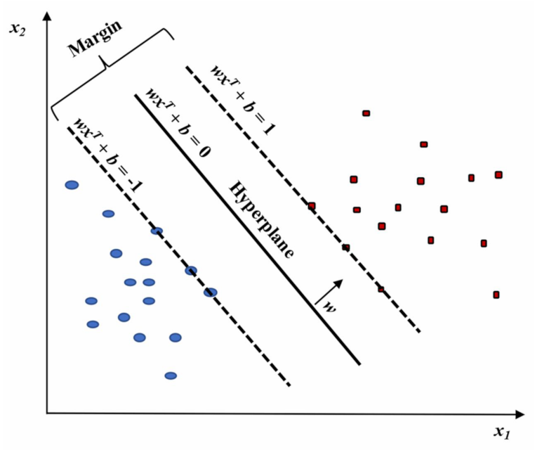
2.2.3. Support Vector Machine (SVM)

Considering the data organized into a matrix, each subject corresponding to a row vector can be conceived as a single point in the p-space of the considered variables. Data can be essentially organized into two main groups, “separated by a gap” whose margins are defined by support vectors. Instead, the edge located in the gap center separating the data corresponds to the dividing hyperplane. SVM tries to define the support vectors, and the prediction will indicate to which hyperplane side the new observations belong. However, generally, data cannot be linearly separated, and hence it is difficult to determine the separating hyperplane. Nevertheless, SVM can accurately execute a non-linear classification throughout the so-called kernel trick. It consists of an implicit mapping of the considered inputs into high-dimensional feature spaces with the objective to their linear separation in that space [68]. In detail, the optimal hyperplane is the one that provides the highest separation between the two classes. With greater definition, by separation, we mean the maximum amplitude (or width, w) between the lines parallel to the hyperplane without any data points in between. This optimal hyperplane is called the maximum-margin hyperplane and the corresponding linear classifier is the maximum-margin classifier (Figure 9).
In addition, in the presence of mislabeled data, the SVM can provide inadequate classifications; therefore, only a few misclassified subjects are found instead by maximizing the separation between the two classes. Finally, validation methods and diagnostic measures are analogous to those adopted in PLS methods. Ultimately, SVM is one of the approaches with the highest accurate prediction, since it is based on statistical learning frameworks [69,70]. It can also be used within machine learning approaches for anomaly detection (such as weather) by choosing an anomaly threshold with the aim to establish whether an observation belongs to the “normal” class or not. Disadvantages of supervised methods include overfitting problems [71] corresponding to the inclusion of noise inside the statistical model. These issues can be provoked by excessive learning, so several validation techniques, such as cross validation [72] or bootstrapping [73], are usually employed to solve them.

2.3. Pathway Analysis Methods

A powerful method to describe peculiar features of the cell metabolism is pathway analysis (PA), which provides a graphical representation of the relationships among the actors (mainly enzymes and metabolites) of precise catalyzed reactions. Therefore, PA is highly employed for the interpretation of high-dimensional molecular data [74]. In fact, taking advantage of the already acquired knowledge of biological pathways, proteins, metabolites and also genes can be mapped onto newly developed pathways with the objective to draw their collective functions and interactions in that specific biological environment [75]. Although PA was initially developed for the interpretation of transcriptomic data, in the last decades, it has become a common method in metabolomics, being particularly suited to find associations between molecules involved in the same biological function for a given phenotype [76,77,78].
PA methods include several tools allowing deep statistical analyses in metabolomics known as enrichment analysis. They grant the functional interpretation of the achieved results mainly in terms of statistically significant pathways [79]. These tools can handle heterogeneous and hierarchical vocabularies and may be classified into two distinct collections. The first encompasses “non-topology-based” (non-TB) approaches, which do not consider the acquired knowledge concerning the character of each metabolite in the considered pathways [80]. Non-TB approaches include the over-representation analysis (ORA) as the first generation technique and the functional class scoring (FCS) as the second generation. Finally, the second collection includes topology-based methods (see Figure 10) that are adopted to determine those pathways that are significantly impacted in a given phenotype.
This latter approach can be classified depending on the considered pathways (e.g., signaling or metabolic), inputs (e.g., subset or all metabolites and metabolites p-values), chosen mathematical models, outputs (e.g., pathway scores and p-values) and the wanted implementation (e.g., web-based or standalone) [81,82]. Note that PA methods were originally developed for genes, but they can be successfully applied for every biomolecule/metabolite [83].

2.3.1. Over-Representation Analysis (ORA)

Over-representation analysis (ORA) is among the most used pathway analysis approaches for the interpretation of metabolomics data needed as input, once the type of annotations to examine is chosen. One obtains a collection of annotations and their associated p-value as outputs since a statistical test is applied to determine whether a set of metabolites is enriched by a specific annotation (e.g., a pathway) in comparison to a background set. Different statistics can be applied to obtain information about the studied biological mechanisms and on the specific functionality of a given metabolite set. Among the most used statistics, we would like to mention the well-known binomial probability, Fisher’s exact test and the hypergeometric distribution [84,85].
Three are the necessary inputs in ORA analysis: (i) a set of pathways (or metabolite collections); (ii) a catalog of investigating metabolites and, (iii) a background collection of compounds. The list of investigating metabolites usually comes from experimental data after applying a statistical test to determine those metabolites whose signals can be associated with a precise result by choosing a threshold value usually associated to the p-values [74]. The background collection includes all metabolites that can be revealed in the considered measurement. If the p-value corresponding to each pathway is obtained by means of the right-tailed Fisher’s exact test based on the hypergeometric distribution, the probability to find k metabolites or more in a pathway can be written as [74]:
P ( X     k )   =   1     i   =   0 k     1 M i N     M n     i N n ,
where N corresponds to the number of background compounds, n is the number of the measured metabolites, M is the number of background metabolites mapping the ith pathway, and k represents the overlap between M and n. A scheme of the ORA principle is displayed in Figure 11 as a 3D Venn diagram. Finally, multiple corrections are usually applied, as calculations are made for many pathways, thus obtaining a collection of significantly enriched pathways (SEP).
Before applying ORA, one has to verify if the metabolomics dataset is sufficiently big to furnish proper statistical significance. For instance, usually MS-based techniques can observe more metabolites than NMR-based methods, such as the mono-dimensional NMR ones commonly used for profiling [86]. Indeed, the choice of the most suitable background collection is the real challenge and still remains an open subject because it strictly depends on the situation [74].

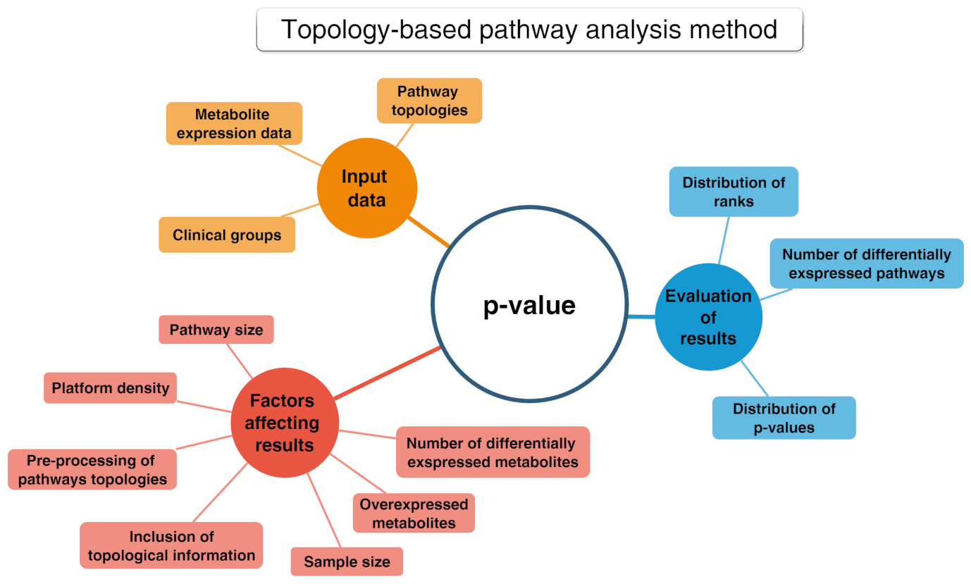
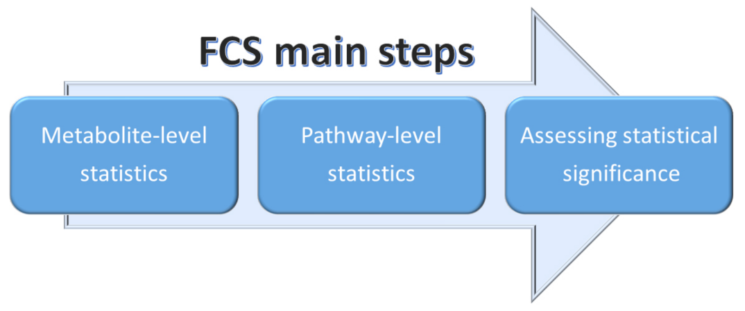
2.3.2. Functional Class Scoring (FCS)

Functional class scoring (FCS) methods look for coordinated variations in the metabolites belonging to a specific pathway. In fact, FCS methods take into account those coordinated changes within the individual set of metabolites that, although weak, can have a significant effect of specific pathways [75,78]. Essentially, all FCS methods comprise three steps (see Figure 12):
  • A statistical approach is applied to compute differential expression of individual metabolites (metabolite-level statistics), looking for correlations of molecular measurements with phenotype [87]. Those mostly used consider the analysis of variance (ANOVA) [88], Q-statistic [89], signal-to-noise ratio [90], t-test [91], and Z-score [92]. The choice of the most suitable statistical approach may depend on the number of biological replicates and on the effect of the metabolites set on a specific pathway [93].
  • Initial statistics for all metabolites of a given pathway are combined into statistics on different pathways (pathway-level statistics) that can consider interdependencies among metabolites (multivariate) [94] or not (univariate) [91]. The pathway-level statistics usually is performed in terms of the Kolmogorov–Smirnov statistics [90], mean or median of metabolite-level statistics [93], the Wilcoxon rank sum [95], and the maxmean statistics [96]. Note that, although multivariate statistics should have more statistical significance, univariate statistics provide the best results if applied to the data of biologic systems (p≤ 0.001) [97].
  • The last FCS step corresponds to estimating the significance of the so-called pathway-level statistics. In detail, the null hypothesis can be tested into two different ways: (i) by permuting metabolite labels for every pathways, so comparing the set of metabolites in that pathway with a set of metabolites not included in that pathway (competitive null hypothesis) [75] and (ii) by permuting class labels for every sample, so comparing the collection of metabolites in a considered pathway with itself, whereas the metabolites excluded by that pathway are not considered (self-contained null hypothesis) [91].

2.3.3. Metabolic Pathway Reconstruction and Simulation

The identification of metabolomic biomarkers and their mapping into a neural network is fundamental to further study the cellular mechanisms and its physiology. The goal is to identify the effects of the metabolites (as a function of their concentration) on the cellular changes, providing a relationship with the most likely biologically meaningful sub-networks. Thus, basing on genome annotation and protein homology, reference pathways could be mapped into a specific organism. However, this mapping method often produces incomplete pathways that need the employment of ab initio metabolomic network construction approaches (such as Bayesian networks), where differential equations describe the changes in a metabolomic network in terms of chemical amounts [98,99]. Qi et al. [100] further improved this approach allowing to optimize accuracy in defining metabolomics features or better the correlation between the substrates whose nature is well known as well as the species of each individual reactions, so defining the classification of the mapped metabolic products in a pathway and their modifications under selected perturbations. Recently, Hu et al. [23] performed a pathway analysis on serum spectra recorded by 1 H NMR with the aim to identify eventual biomarkers characterizing the treatment of human lung cancer. After a first statistical analysis in terms of PLS-DA, they were able to identify four metabolic pathways associated with the metabolic perturbation induced by non-small-cell lung cancer (Figure 13) by means of the MetaboAnalyst package [101]. In detail, the highest pathway impact was shown by the metabolisms of (i) taurine and hypotaurine, (ii) d-glutamine and d-glutamate, (iii) glycine, serine and threonine, and (iv) alanine, aspartate and glutamate, thus shedding light on the responsible processes in this kind of cancer.

3. Artificial Intelligence toward Learning Techniques

Artificial intelligence (AI) techniques are based on algorithms that try to simulate both human learning and decision making. Indeed, AI exploits the ability of computer algorithms to learn from a given dataset containing precise information that then must be recognized in new dataset in an automatic way. Specifically, the computer algorithms during learning on the test dataset create models that are able to provide information on the probability that a specific result may occur. Furthermore, these programs are usually able to identify the important features associated with the outcome of interest. Artificial intelligence methods can accurately handle big data for biomarkers prediction, allowing the determination of relevant characteristics pertaining to a dataset and a deep comprehension of the significance of such data. Specifically, the integration of metabolic snapshots with metabolic fluxes and the use of knowledge-informed AI methods allow obtaining a profound comprehension of metabolic pathways at the system level. Hence, the development of multi-omic techniques integrating both experimental and computational methods, adequate to extract metabolic information at the cellular and subcellular levels, will provide powerful tools to enter the details of metabolic (dis)regulation, therefore allowing the exploitation of personalized therapies [102].

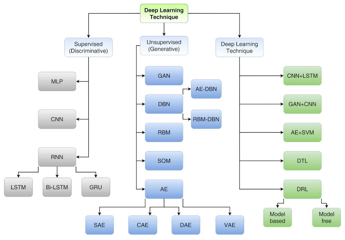
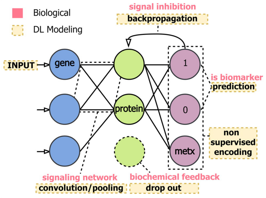
Machine Learning, Neural Networks and Deep Learning

All the conventional approaches discussed in the previous sections can be implemented by learning algorithms that let the corresponding network learn by a given dataset and, after performing a test with a sample dataset, can be used with a known predictive power. In this section, we get into details of the different machine learning techniques as a subset of AI methods (Figure 14).
In addition, neural networks and deep learning approaches are characterized in terms of the number of node layers, also named depth. Briefly, a node is the locus in which the algorithm performs the calculation and would correspond to the action that a neuron exerts in the human brain when it is subject to a stimulus. As shown in Figure 15b, a node takes different inputs, each having its own weight, that can be amplified or reduced by the activation function, thus giving a corresponding significance to the received inputs with respect to the specific task that the used algorithm is learning. So, a neural network consisting of two or more hidden layers can be classified as a deep learning technique and is usually described by the diagram shown in Figure 15a, together with a scheme of how one node might look (Figure 15b).
Deep learning techniques, being able to handle large datasets, thus allowing a high-level description, are already used to provide the optimal route to solve a lot of issues in the field of image recognition, speech recognition, and natural language processing. Furthermore, DL techniques can be divided into three main categories (see Figure 16) that are deepened in Ref. [104]:
  • Supervised learning (discriminative) includes multi-layer perceptron (MLP), convolutional neural network (CNN), long short-term memory (LSTM) and gated recurrent unit (GRU);
  • Unsupervised learning (generative) includes generative adversarial network (GAN), autoencoder (AE), sparse autoencoder (SAE), denoising autoencoder (DAE), contractive autoencoder (CAE), variational autoencoder (VAE), self-organizing map (SOM), restricted Boltzmann machine (RBM) and deep belief network (DBN);
  • Hybrid learning (both discriminative and generative) includes models composed by both supervised and unsupervised algorithms other than deep transfer learning (DTL) and deep reinforcement learning (DRL).
Supervised learning can furnish a discriminative function in classification applications by identifying the different features of those classes that can be extracted by the data. Among them, multi-layer perceptron (MLP) is a feedforward ANN that involves (i) an input layer collecting input signals, (ii) an output layer that provides an outcome in consideration of the processed input and (iii) some hidden layers separating the input and output layers that correspond to the network computational engine. On the contrary, unsupervised learning is employed to recognize eventual correlations by analyzing the signals pattern and to assess the statistical distributions of the achieved results both on original data and on their corresponding classes. This kind of generative approach can be also used as an initial step (pre-processing) before applying supervised learning methods. Most common unsupervised techniques, reported in Figure 16, are listed and briefly described in the next. Hybrid learning paradigms combining both discriminative and generative methods are possible. Hybrid deep learning architectures are usually constituted by multiple models where the basis can indeed be either a supervised or unsupervised deep learning method. Common hybrid learning algorithms are, for example, semi-supervised learning that allows to use a supervision for some data points, keeping the others unlabeled, and deep reinforcement learning (DRL; see Figure 16) that, interacting with an environment, involves the knowledge of performing with sequential decision-making tasks in order to maximize cumulative rewards [104,105]. Their advantages lie in the possibility to consider the best aspects of discriminative and generative models. For instance, a hybrid architecture can adopt small inputs to avoid the problem of determining the right network size and instead an increasing number of neurons in receptive-field spaces [106]. At the same time, by a proper enhancement of the initial weights through suitable algorithms, neural networks in hybrid architectures can provide higher accuracy and predictive power [107,108].
Most of the techniques in the categories indicated before are feed-forward (working from input to output) but, as detailed in the last part of the section, the opposite movement is also possible. This is called backpropagation and works from output to input, allowing the evaluation of the individual neuron’s error, allowing to properly modify and fit the algorithm iteratively. Unlike ML, that usually adopts manual identification and description of relevant features, DL techniques aim to execute automatically the features extraction, avoiding almost all human participation. In addition, DL can handle larger datasets, especially of the unstructured type. In fact, DL methods can have unstructured raw data as input (such as text or images) and can directly define which characteristics must be considered to distinguish the original observations. By recognizing similar and/or different patterns, DL methods can adequately cluster inputs. Therefore, DL approaches would need a very high number of observations to be as accurate as possible. Generally, and according to the scheme reported in Figure 16, the most adopted deep learning techniques are the following [104]:
1.
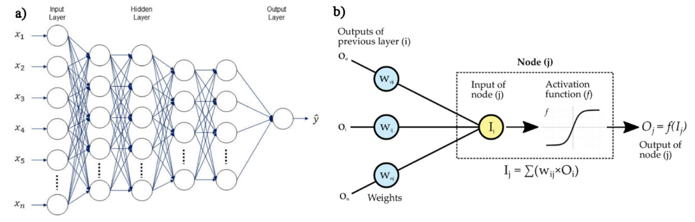
Classic neural networks encompass linear and non-linear functions which, in turn, include S-shaped functions ranging from 0 to 1 (sigmoid) or from −1 to 1 (hyperbolic tangent, tanh) and rectified linear unit (ReLU), which gives 0 for input lower than the set value or evaluates a linear multiple for bigger input.
2.
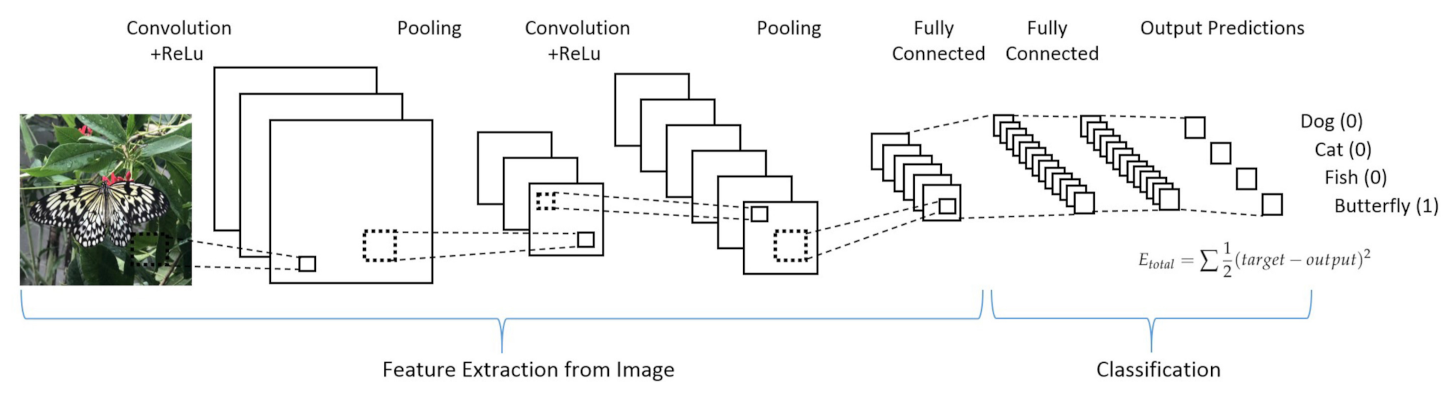
Convolutional neural networks (CNN) take into high consideration the neuron organization found in the visual cortex of an animal brain. It is particularly suited for high complexity and allows for optimal pre-processing. Four stages can be considered for CNN building (see Figure 17):
(a)
Deduce feature maps from input after applying a proper function (convolution);
(b)
Reveal an image after given changes (max-pooling);
(c)
Flatten the data for the CNN analysis (flattening);
(d)
Compiling the loss function by a hidden layer (full connection).
3.
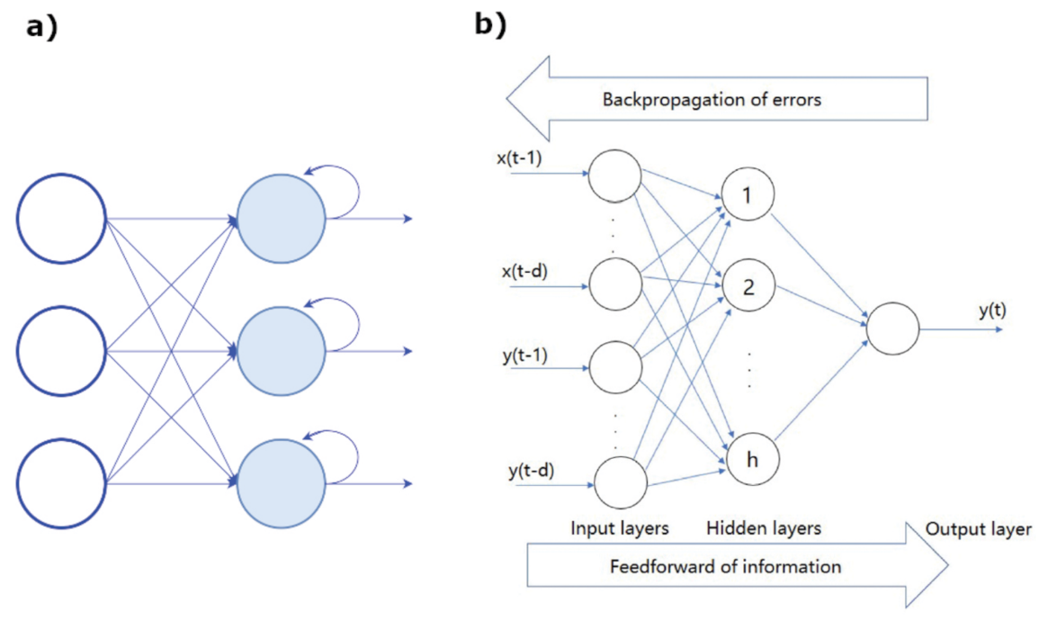
Recurrent neural networks (RNN) are exploited when the objective is the prediction of a sequence. They are a subset of ANN for sequential or time series data, usually applied for language translation, speech recognition, and son on. Their peculiar feature is that the outcome of the output node is a function of the output of previous elements within the sequence (see Figure 18a).
4.
Generative adversarial networks (GAN) combine generator networks for providing artificial data and discriminator networks for distinguishing real and fake data.
5.
Self-organizing maps (SOMs) have a fixed bi-dimensional output since each synapse joins its input and output nodes, and usually take advantage of data reduction performed by unsupervised approaches.
6.
Boltzmann machine is a stochastic model exploited for yielding proper parameters defined in the model.
7.
Deep reinforcement learning are mainly used to understand and so predict the effect of every action executed in a defined state of the observation.
8.
Autoencoders work directly on the considered inputs, without taking into account the effect of activation functions. Among the autoencoders, we mention the following:
(a)
Sparse autoencoders have more hidden than input layers for reducing overfitting.
(b)
Denoising autoencoders are able to reconstruct corrupted data by randomly assigning 0 to some inputs.
(c)
Contractive autoencoders include a penalty factor to the loss function to prevent overfitting and data repetition when the network has more hidden than input layers.
(d)
Stacked autoencoders perform two stages of encoding by the inclusion of an additional hidden layer.
9.
Backpropagation (BP) are neural networks that use the flux of information going from the output to input for learning about the errors corresponding to the achieved prediction. An architecture of the BP network is shown in Figure 18b.
10.
Gradient descent are neural networks that identify a slope corresponding to a relation among variables (for example, the error produced in the neural network and data parameter: small data changes provoke errors variations).
From the above brief information, it emerges that, even if DL methods can be thought as black-box solutions, future generation deep learning can provide a great aid for the analysis of big data and for corresponding reliable results.

4. Applications of Deep Learning Approaches for NMR-Based Metabolomics

In this section, the applications of deep learning on NMR-based metabolic data for specific different fields are reported and discussed. Here, we briefly introduce the potentiality of the applications of deep learning in metabolomics which today are still relatively low compared to other omics. This is explained since metabolome-specific deep learning architectures should be defined, and dimensionality problems and model evaluation regime should be further evaluated. In any case, data pre-processing using convolutional neural network architecture appears to be the most efficient approach among the deep learning ones. The main advantage of CNNs compared to a traditional neural network is that they automatically detect important features without any human supervision. Specifically, CNNs learn relevant features from image/video at different levels, similar to a human brain [110]. This is very relevant to analyze both biomedical and food data, whose classification in view of safety security actions is extremely important.
The potentiality of the NMR technique within the field of metabolomics is currently employed for several purposes, including the detection of viable microbes in microbial food safety [10], the assessment of aquatic living organisms subjected to contaminated water [111], the identification of novel biomarkers to diagnose cancer diseases [112] and the monitoring of the plant growth status changing environmental parameters in view of smart agriculture [113]. In the next sections, we discuss some applications of deep learning approaches for NMR-based metabolomics in food and biomedical areas, highlighting their strengths and limitations.
Even before the development of artificial intelligence, statistical analyses were successfully applied in food analysis but with some limitations. For example, traditional methods are usually not very accurate in the classification of similar foods in contrast to modern deep learning approaches that allow enhancing all small differences. However, traditional methods usually constitute the first step, providing the input for neural networks with the aim to achieve a more accurate and automatic output. Furthermore, advanced computational algorithms can be applied not only for statistical analysis, but also to execute simulations whose predictions depend on the considered conditions [114].

4.1. Food

Foodomics is a term referred to the metabolomic approaches applied to foodstuffs for investigating topics mainly related with nutrition. Nowadays, DL methods are being progressively applied in the food field with different purposes, such as fraud detection [115]. Furthermore, another important issue is to guarantee the geographical origin and production/processing procedures of food, the precise proportions of ingredients, including additives and the kind of used raw materials. In this context, machine learning is a powerful method for achieving an adequate classification. For example, Greer et al. [116] carried out NMR measurements using a not-conventional protocol to measure the magnetization relaxation times (both the longitudinal T 1 and transverse T 2 ) and then they efficiently classified cooking oils, milk, and soy sauces (see Figure 19).
Since the considered datasets are very large (typically about 5 × 10 6 points each), the authors first reduced their size by means of the singular value decomposition, thus allowing a fast classification and also providing little insight into the sample physical properties. Figure 19 reports different combinations for the obtained classification features. Figure 19a,b corresponds to the two components used by the Gaussian fit of those peaks revealed by the inverse 2D Laplace transform [117]. A sharp distinction of the samples is clearly shown for every adopted combination. The y-axes of Figure 19a,c report the first component of T 1 versus the first and second components of T 2 , respectively. Contrarily, the y-axes of Figure 19b,d report the second component of T 1 versus the first and second components of T 2 , respectively. The authors found that most of the trained models reached an accuracy up to 100% (see, for example, Figure 20a). Finally, they also pointed out the effect of the sample temperature on classification accuracy for achieving reliable results (see Figure 20b).
Nowadays, deep neural networks (DNNs) are rarely used for metabolomics studies because the assignment of metabolites contribution in NMR spectra still lacks highly reliable yields due to the complexity of the investigated biological matrix and thus of the corresponding signals. As described in the previous section, different deep learning methods were used, but some of them are characterized by some limitations (i.e., low accuracy in classification). Some efforts were made to overcome this problem. Date et al. [118] recently developed a DNN method that includes the evaluation of the so-called mean decrease accuracy (MDA) to estimate every variable. It relies on a permutation algorithm that allows the recognition of the sample geographical origins and the identification of their biomarkers. On the other hand, for food authenticity and nutritional quality, the fast revelation of viable microbes is still a challenge. Here, we report a multilayer ANN example (see Figure 21) showing four input neurons, two hidden layers made of three neurons, and two output neurons.
Such a scheme was organized by Wang et al. [119] for the detection, by means of NMR spectroscopy coupled with deep ANNs, of pathogenic and non-pathogenic microbes. According to the classification method, each output neuron is associated to one possible output. Here, “Salmonella” shows the highest value of output, thus corresponding to the prediction performed by the used ANN. In such a case, the weights of each input are optimized to reach the wanted outcome throughout back propagation, thus defining multiple epochs and training cycles. Figure 22 reports an example referred to an ANN analysis with two hidden layers of 800 neurons. ANN training is made optimizing a set of training criteria to avoid shallow local minima. In particular, training continues when the loss function decreases after an epoch of training (“greedy” algorithm—case a) and even after a small increase followed by a continuous decrease (case b). On the contrary, training stops for an increase in the loss function after several constant values (case c) and for steep increases (case d) [119].
Once the network is trained, it is able to perform predictions on new input data. As already mentioned, the loss and the model accuracy provide a measure of the output goodness. In fact, the aim is to minimize the disagreement between the prediction and the reality (loss) and to maximize accuracy (cross-validation method). Thanks to this approach, Wang et al. [119] found that the used ANNs accurately predict 91.2% of unknown microbes and, after repeating the model training by considering just those metabolites whose amount increased with incubation time, they observed an accuracy up to 99.2%.
Machine learning and neural network approaches are simultaneously adopted to analyze large amounts of NMR metabolomics data for food safety [109]. This can be performed also by means of magnetic resonance imaging (MRI), which is an imaging technique relying on NMR principles. Within the food field, it is mainly used to resolve the tissue texture of foods [120,121]. On the other hand, Teimouri et al. [122] used PLSR, LDA, and ANN for the classification of the data collected by CCD images from food portions, different in color and geometrical aspects. In this way, they were able to classify 2800 food samples in one hour, with an overall accuracy of 93%. Instead, De Sousa Ribeiro et al. [123] developed a CNN approach able to reconstruct degraded information on the label of food packaging. Before applying CNNs, they started with K-means clustering and KNN classification algorithms for the extraction of suitable centroids.

4.2. Biomedical

Metabolomics-based NMR investigations, coupled with deep learning methods, are increasingly employed within the biomedical field. More profoundly, the use of complex DL architectures hardly allows achieving a predictive power with ranking or selection. As already discussed, DL models use several computational layers to analyze input signals and establish any eventual preferred direction for signal encoding (forward or backward). This procedure does not usually allow the interpretation of input signals in terms of the used model, making it hard to identify biomarkers in a network, where biological and DL modeling are connected (Figure 23).
Today, it is still necessary to uniform assessment metric for biomedical data classification or prediction, also avoiding false negatives in disease diagnosis. Further, deep learning is a promising methodology to treat data collecting by smart wearable sensors, which is considered fundamental in epidemic prediction, disease prevention, and clinical decision making, thus allowing a significant improvement in the quality of life [124,125].
With the aim to obtain an accurate metabolites identification from the observation of the corresponding peaks in complex mixtures, Kim et al. [126] developed a convolutional neural network (CNN) model, called SMART-Miner, which is trained on 657 chemical entities collected from HMDB and BMRB databases. After training, the model is able to automatically carry out the recognition of metabolites from 1 H- 13 C HSQC NMR spectra of complex metabolite mixtures, showing higher performance in comparison with other NMR-based metabolomic tools (Figure 24).
Brougham et al. [127], by employing ANNs on 1 H NMR spectra, performed a successful classification of four lung carcinoma cell lines, showing different drug-resistance patterns. The authors chose human lung carcinoma and adenocarcinoma cell lines together with specific drug-resistant daughter lines (Figure 25). The ANN architecture was constructed at first using three layers and the corresponding weights were determined by minimizing the root mean square error. Then, the authors analyzed networks with four layers, two of which are hidden. Their results show that the four-layer structure with two hidden layers provided a 100% successful classification [127]. These data are very interesting in terms of the robustness of the used approach: the cell lines were correctly classified, even though the effects were provoked by the operator and independently from the spectra chosen for training and validation (Figure 25).
Very recently, Di Donato et al. [128] analyzed serum samples from 94 elderly patients with early stage colorectal cancer and 75 elderly patients with metastatic colorectal cancer. With the aim to separately observe each different molecular components, these authors acquired one-dimensional proton NMR spectra by using three different pulse sequences for each sample: (i) a nuclear Overhauser effect spectroscopy pulse sequence to observe molecules with both low and high molecular weight; (ii) a common spin echo mono-dimensional pulse sequence [129] to observe only lighter metabolites and (iii) a common diffusion-edited pulse sequence to observe only macromolecules [128]. Their results, taking advantage of Kaplan–Meier curves for prognosis and of a PCA-based kNN analysis, allowed distinguishing relapse-free and metastatic cancer groups, with the advantage of obtaining information about the risks in the early stage of the colorectal cancer disease.
Peng et al. [130], by using two-dimensional NMR correlational spectroscopy on the longitudinal (T 1 ) and transversal components (T 2 ) of the magnetization relaxation time during its equilibrium recovery, were able to perform a molecular phenotyping of blood with the employment of supervised learning models, including neural networks. In detail, by means of a fast two-dimensional Laplace inversion [117], they obtained T 1 –T 2 correlation spectra on a single drop of blood (<5 μ L) in a few minutes (Figure 26) with a benchtop-sized NMR spectrometer. Then, they converted the NMR correlational maps for deep image analysis, achieving useful insights for medical decision making by the application of machine learning techniques. In particular, after an initial dimensionality reduction by unsupervised analysis, supervised neural network models were applied to train and predict the data that, at the end, were compared with the diagnostic prediction made by humans. The results showed that ML approaches outperformed the human being and took a much shorter time. Therefore, the authors demonstrated the clinical efficacy of this technique by analyzing human blood in different physiological and pathological conditions, such as oxidation states [130]. Concerning the analysis of different physiological conditions, Figure 26 reports the T 1 –T 2 correlational maps of blood cells at oxygenated (a), oxidized (b), and deoxygenated (c) states. Three peaks with different relaxation times values were observed and assigned to the different microenvironments that water experiences in the considered samples of red blood cells. For the obtained maps, the coordinate for the bulk water peak (slowest component) is shown at the upper left of the map indicating T 2 and T 1 relaxations (in ms) and T 1 /T 2 -ratio, respectively. Instead, the coordinates of the fastest components, due to hydration and bound water molecules [131], are reported close to the corresponding correlation peak (Figure 26).

5. Conclusions and Future Perspective

The role played by each metabolite (in terms of identification and quantification) is essential to validate NMR spectroscopy potentiality in this field. Overall, NMR-based metabolomics coupled with machine learning and neural networks improves its power, especially in the food and biomedical fields, paving the way for innovative and hybrid approaches for deep insights into the metabolic fingerprinting of complex biological matrices. In fact, the number of identified metabolites is very low, and in some cases, the metabolites profile analysis is difficult for the high noise level and the multicolinearity with respect to the genomics case. However, the coupling of genomics and metabolomics tools is still a goal to be achieved. To this purpose, the deep learning and neural network approaches are the best methods to use, although the first step may involve the use of linear discriminant analysis to select a subset of metabolites to be used as input for the neural network analysis in view of an accurate classification as well as the generalizability of the method. Therefore, some efforts are still necessary for applying deep learning approaches on NMR metabolomics data, strictly related to the specific properties of the selected/investigated metabolites, evaluating the dimensionality reduction problems and improving the reliability of the evaluation models.

Author Contributions

Conceptualization, C.C., F.N. and E.F.; methodology, S.V., A.M.M. and G.N.; writing—review and editing, all authors. All authors have read and agreed to the published version of the manuscript.

Funding

This research received no external funding.

Institutional Review Board Statement

Not applicable.

Informed Consent Statement

Not applicable.

Data Availability Statement

No new data were created or analyzed in this study, so data sharing is not applicable to this article.

Conflicts of Interest

The authors declare no conflict of interest.

Abbreviations

The following abbreviations are used in this manuscript:
NMRNuclear Magnetic Resonance
MSMass Spectrometry
AIArtificial Intelligence
MLMachine Learning
DLDeep Learning
NNNeural Network
ANNArtificial Neural Network
DNNDeep Neural Network
PCAPrincipal Component Analysis
PLSPartial Least Squares
ORAOver Representation Analysis
FCSFunctional Class Scoring

Appendix A. Technical Aspects

Nuclear magnetic resonance (NMR) is one of the most employed experimental techniques for investigating the wide composition and structural complexity of biological samples. The NMR technique is characterized by high reproducibility and ease of sample preparation and measurement proceedings. NMR is a non-destructive technique able to perform different measurements on the same sample, providing increasingly accurate and detailed information. NMR also allows to reach a quantitative analysis and to carry out in vivo metabolomics studies. Unfortunately, it has a relatively low sensitivity ( μ M), but, in combination with chromatography, it shows a great potentiality for targeted analysis. However, it is a relatively young experimental technique with continuous development from both the hardware and software point of view (see Ref. [3] for a more details). For instance, cryoprobes [132,133,134] and magic angle techniques [17,135,136] are today commonly used for improving the signal-to-noise ratio, while AI methods are used both for signal pre-processing, such as baseline optimization [137,138,139], and for data analysis, as discussed in the main text of this review.
Briefly, the NMR working principle is based on the resonant excitation of the precession dynamics of the nuclear magnetic moment under the effect of a static magnetic field. Nuclei characterized by an odd number of protons and/or neutrons show a magnetic moment, associated to the nuclear spin characterized by the corresponding quantum number (I). Nuclei with I ≠ 0 possess an intrinsic nuclear magnetic moment ( μ ) so producing a slight local magnetic field (B 0 ). Once immersed in an external magnetic field (B), these nuclei, previously randomly orientated, align themselves either in the same or opposite direction of B. These nuclei, subject to B, move in a precessional motion at a frequency called Larmor frequency, which takes on values in the range of 50–900 MHz (see Figure A1). Indeed, it is characteristic for each nucleus and increases with the strength of the external magnetic field B. In this condition, if the system is irradiated with an electromagnetic radiation at the corresponding Larmor frequency (resonance condition), nuclei can absorb the radiation energy, and the nuclear spins can be promoted to a different Zeeman level.
Figure A1. (A) Spectroscopies and corresponding frequency ranges. Larmor frequency of most used nuclei for metabolomics analyses with respect to that of the proton when at 600 MHz. (B) Parts per million intervals for all these nuclei ( 15 N, 13 C, 31 P, 19 F and 1 H) at characteristic chemical environments. Figure reprinted from Ref. [3] under the terms of the Creative Common CC-BY license.
Applsci 12 02824 g0a1
When spins relax toward the fundamental state, they emit a radio frequency (damped in time, called free induction decay (FID)) that well characterizes each nucleus of the system, depending on the corresponding chemical environment that essentially exerts a local magnetic field, causing a shift (chemical shift) from the pure Larmor frequency value. This is commonly indicated by δ and measured in parts per million since the recorded frequency is divided by the spectrometer working frequency such that the spectra acquired with different instruments can be compared. Note that nuclei with I = 0, such as 12 C and 16 O, are NMR inactive [140,141].
Figure A1B reports the most common NMR active nuclei. Among them, 13 C and 15 N show a wide chemical shift range, together with a sharp line signal, but their poor natural abundance and the low sensitivity (compared to other nuclei as 1 H or 19 F) limit their employment in the metabolomic investigation. 31 P has a good sensitivity (6.6 × 10 2 relative to 1 H) and a wide spectral range, but only few metabolites, such as nucleoside or phospholipids, contain it, restricting its employment to a few compounds. The same comments can be done about 19 F.
The high abundance in nature, high sensitivity and relevant gyromagnetic ratio of 1 H makes 1D 1 H NMR spectra especially useful in the metabolomic investigation. The 1D 1 H NMR spectra are fast to record (few minutes) and just the information contained in only one spectrum can provide useful data to identify and quantify from 50 to 100 metabolites [142,143]. In this case, if nuclear spins are totally relaxed and no polarization transfer sequences are applied, the intensity of each acquired proton signal is correlated with the corresponding concentration levels in the molecules, and the area under each peak is directly proportional to the number of 1 H constituting the corresponding residue, giving a real distribution of the individual metabolites in the sample mixture. This quantification is possible without previous calibration, thanks to the large linear dynamic range and signal response that characterize proton NMR spectroscopy.
Another important aspect in the analysis of the 1 H NMR spectra is the solvent suppression, and in this way, several protocols can be used. Commonly, the protonated solvent can be replaced with a deuterated one; this procedure can also require the lyophilization of the sample and the subsequent dispersion in the deuterated solvent. When this is not possible, the solvent peak can be suppressed by using proper pulse sequences [144]. Regarding the identification of metabolites constituting a biological matrix, when they have a unique and high reproducible fingerprint at specific conditions (pH, solvent, temperature), the non-target strategy can be adopted [145]. This consists of the employment of multimodal models, which clarify how the NMR fingerprint of each sample and among the groups correlate with each other, providing a static analysis. This strategy is very important to give a first overview about the sample composition; however, it is not sufficient to analyze very complex samples. In the latter case, it is more common to adopt the target strategy, which consists in the comparison of the acquired data with available metabolite databases, such as the Human Metabolome Database, Biological Magnetic Resonance Data Bank, Birmingham Metabolite Library, Bbiorefcode (Bruker Biospin Ltd., Billerica, MA, USA) and Chenomx library (Chenomx Inc., Edmonton, AB, USA) [145].
Figure A2 reports a 1 H NMR spectrum acquired from human serum at 700 MHz: 55 different metabolites were identified and labeled in the recorded spectrum [3]. In particular, each proton signal can be attributed to the different components of the biofluid, thanks to the high sensitivity of 1 H nuclei, its natural abundance and the remarkably narrow line widths, giving a remarkable spectrum resolution. Note that the high intensity of the lactate peak is due to a conversion of the glucose in lactate during the preparation of the sample. To reach a certain assignment of the detected metabolic peaks 1D 1 H NMR is sometimes not sufficient. This is due to the relevant numbers of resonances with an ambiguous assignment, and to a peak overlap of the matrix’s components. Thus, bi-dimensional (2D) NMR techniques, which investigate the spin–spin correlation among 1 H- 1 H nuclei or with heteroatoms, such as 13 C, 15 N, 31 P, are adopted. In metabolomic studies, typical 2D NMR techniques are 1 H- 1 H correlated spectroscopy (COSY) and total correlation spectroscopy (TOCSY), 1 H- 13 C heteronuclear single quantum coherence (HSQC) and heteronuclear multiple bond correlation (HMBC). HSQC is a great experiment for metabolites identification, which gives information on the direct connectivity between protons and heteroatoms. In particular, the large chemical shift scale of 13 C helps to solve the tough issue of the overlapped signals in the proton spectrum, and the variety of HSQC experiments can provide different sets of information on the investigated sample.
For instance, the potentiality of the HSQC technique was proved in the identification of methyl groups of betaine and trimethylamine-N-oxide (TMAO). The proton resonances of methyl groups in TMAO and betaine organic compounds are both close to δ = 3.26 ppm, and thus, the signals are not distinguishable. Instead, the carbon chemical shift of methyl groups in TMAO is assigned at 62.2 ppm, while that of betaine is at 55.8 ppm. This information can be easily obtained by the 1 H- 13 C HSQC experiment (see Figure A3), giving an unambiguous identification of the two organic compounds [145]. HMBC is an appropriate technique to analyze the correlations using the coupling of protons with heteroatoms, which are separated up to four bonds, providing complementary information to that given by HSQC for the structural characterization of metabolites.
Figure A2. 1 H NMR spectrum of ultrafiltered human serum at 700 MHz with the identified compounds labeled above each of the corresponding peaks. Figure reprinted from Ref. [3] under the terms of the Creative Common CC-BY license.
Applsci 12 02824 g0a2
Figure A3. 1 H- 13 C 2D HSQC experiment to identify TMAO and betaine organic compounds of a biological matrix. Figure reprinted from Ref. [145] under the terms of the Creative Common CC-BY license.
Applsci 12 02824 g0a3
Thus, metabolic identification can be easily reached by the combination of 2D-NMR techniques with the metabolite databases. However, in some cases, the concentration of metabolites is very low, and their peaks are often overlapped making their identification difficult, even when employing 2D NMR techniques. In these cases, if the sharp chemical shift of the compounds to identify is known, it is recommended to use a standard (reference) compound, which is added in the concentration range 10–100 μ M. For instance, this method was applied to identify the uridine diphosphate (UDP) conjugates, which are present in very low concentrations in cellular extracts with overlapped peaks, but their chemical shift is well known and the signal-to-noise ratio (S/N) has sufficient intensity to be quantified by 1D/2D NMR experiments [145]. Figure A4 shows in details how the spiking of pure compounds into a mixture aids the identification of metabolites within the spectrum and also its quantification by performing peak fitting of the two spectral regions corresponding to UDP-nacetylglucosamin (UDP-Gluc-NAc). Note that the proton signal on the left side ( δ = 5.50 ppm) of UDP-Gluc-NAc is overlapped to that of galactose-1-phosphate (Gal-1-P), whereas signals from the uridine group ( δ = 5.95 ppm) superimpose with those from UDP-glucose. In addition, without spiking, it is almost impossible to define the shift of the methyl group belonging to UDP-Gluc-Nac acetyl (right region) since there is a big overlap with other signals, such as the multiplets from glutamine and glutamate.
The addition of a standard is also employed to obtain an absolute quantification of the metabolites contained in the sample. Therefore, the estimation of the metabolites concentration can be made by comparing the area of the metabolites NMR peaks with that of the reference sample by the following equation:
M S = I m I s   ×   N s N m
in which M and S represent the amounts of the considered metabolite and that of the reference, while Im and Is indicate the area under the curve of corresponding peaks, and Nm and Ns represent the number of protons which contribute to these bands, respectively [145]. To quantify a small set of metabolites whose resonances are well-resolved peaks, also the pulse length-based concentration determination (PULCON) quantitative NMR can be used. It considers that the signal intensity is inversely proportional to the duration of the 90 pulse adopted to excite nuclei [146].
Figure A4. (A): The spiking of UDP-nacetylglucosamine (UDP-Gluc-NAc) allows its identification and quantitation. (B): The same spectrum of A without the addition of UDP-Gluc-NAc. Figure reprinted from Ref. [145] under the terms of the Creative Common CC-BY license.
Applsci 12 02824 g0a4
Finally, another possibility for quantitative NMR analysis was reached by using a digital standard electronic reference to access in vivo concentration (ERETIC) technique [147]. It consists of the generation of a signal via a second channel of the probe and the addition of it as a pseudo-FID during the acquisition of the proton experiment, resulting in a common NMR signal [148]. Initially, the ERETIC technique required to be calibrated before running the quantification measurements and some hardware rearrangements. Improvements of ERETIC are ERETIC2 (Bruker Biospin, Topspin 3.0) and quantification by artificial signal (QUANTAS) [149].
Considering the complexity of NMR spectrum of metabolites, often, peak integration is not a sufficient method for the quantitative estimation, and in these cases, the deconvolution approach is preferred. It consists in the fit of a target peak of the compound by using the signal acquired from the reference compound [150]. Different specific software for NMR, such as TopSpin (Bruker), MNova (Mestrelab Research), Spectrus Processor (ACD/Labs), Delta (JEOL) and Chenomx NMR Suite (Chenomx Inc.) can be used for this goal. Among them, JEOL Delta is the only one completely free of charge, while Chenomx NMR Suite seems to show the best performance because it is based on a sophisticated targeted profiling technology and on reference libraries containing hundreds of metabolite spectral data, allowing a user-friendly deconvolution of complex NMR spectra [151]. The spectral analysis and deconvolution can also be performed with non-specific software, such as Matlab (The MathWorks, Inc.) or R (The R Foundation).
Several factors (i.e., pulse sequence changes or variation in the repetition time) influence the deconvolution process and its accuracy, including the variety of standard compounds present in the library and the need to repeat the NMR data acquisition in the same experimental conditions. Changes in the pulse sequence and/or the repetition time result in a less accurate fitting. The performance of the deconvolution is also influenced by the protons’ bond to nitrogen atoms, also called labile (for instance, the α -protons in amino acids) [145]. These protons fast exchange with the solvent, and this not only makes it difficult to detect them, but also provokes changes in the line shape of the close protons peaks. The result is an attenuated resonance, which does not precisely match with the integral corresponding to the other proton peaks in the considered sample. Another error regards the partial peak saturation of the protons, with a resonance close to the presaturation peak of the solvent (commonly water). This was observed for the anomeric protons of carbohydrates, which are frequently resonant close to the water signal, or also for the CH quartet at δ 4.11 ppm in the lactate spectrum. Beyond these disadvantages, the deconvolution approach is a great and widely employed tool for the metabolomic quantification studies [145].
Generally, successful NMR metabolomics requires statistical analyses, which have become progressively advanced over the years, and are the focus of this review. Dependent and independent parameters are correlated by means of conventional approaches on the basis of the mathematical relationship and, in turn, on model fitting. On the other hand, machine learning approaches group input data based on a cluster classification without any statistical assumption, while deep learning is devoted to find statistical inferences from a large amount of input data. The future of NMR-based metabolomics is to generalize the learning approaches to optimize predictive ability for specific diseases.

References

  1. Muthubharathi, B.C.; Gowripriya, T.; Balamurugan, K. Metabolomics: Small molecules that matter more. Mol. Omics 2021, 17, 210–229. [Google Scholar] [CrossRef] [PubMed]
  2. Zhu, M.; Du, X.; Xu, H.; Yang, S.; Wang, C.; Zhu, Y.; Zhang, T.; Zhao, W. Metabolic profiling of liver and faeces in mice infected with echinococcosis. Parasites Vectors 2021, 14, 324. [Google Scholar] [CrossRef] [PubMed]
  3. Emwas, A.H.; Roy, R.; McKay, R.T.; Tenori, L.; Saccenti, E.; Gowda, G.A.N.; Raftery, D.; Alahmari, F.; Jaremko, L.; Jaremko, M.; et al. NMR Spectroscopy for Metabolomics Research. Metabolites 2019, 9, 123. [Google Scholar] [CrossRef] [PubMed] [Green Version]
  4. Onuh, J.O.; Qiu, H. Metabolic Profiling and Metabolites Fingerprints in Human Hypertension: Discovery and Potential. Metabolites 2021, 11, 687. [Google Scholar] [CrossRef]
  5. Caspani, G.; Sebők, V.; Sultana, N.; Swann, J.R.; Bailey, A. Metabolic phenotyping of opioid and psychostimulant addiction: A novel approach for biomarker discovery and biochemical understanding of the disorder. Br. J. Pharmacol. 2021, 1–29. [Google Scholar] [CrossRef]
  6. Wishart, D.S.; Guo, A.; Oler, E.; Wang, F.; Anjum, A.; Peters, H.; Dizon, R.; Sayeeda, Z.; Tian, S.; Lee, B.L.; et al. HMDB 5.0: The Human Metabolome Database for 2022. Nucleic Acids Res. 2022, 50, D622–D631. [Google Scholar] [CrossRef]
  7. Ulrich, E.L.; Akutsu, H.; Doreleijers, J.F.; Harano, Y.; Ioannidis, Y.E.; Lin, J.; Livny, M.; Mading, S.; Maziuk, D.; Miller, Z.; et al. BioMagResBank. Nucleic Acids Res. 2007, 36, D402–D408. [Google Scholar] [CrossRef] [Green Version]
  8. Goodacre, R.; Broadhurst, D.; Smilde, A.K.; Kristal, B.S.; Baker, J.D.; Beger, R.; Bessant, C.; Connor, S.; Capuani, G.; Craig, A.; et al. Proposed minimum reporting standards for data analysis in metabolomics. Metabolomics 2007, 3, 231–241. [Google Scholar] [CrossRef]
  9. Claridge, T.D. High-Resolution NMR Techniques in Organic Chemistry; Elsevier: Amsterdam, The Netherlands, 2016. [Google Scholar] [CrossRef]
  10. Oyedeji, A.B.; Green, E.; Adebiyi, J.A.; Ogundele, O.M.; Gbashi, S.; Adefisoye, M.A.; Oyeyinka, S.A.; Adebo, O.A. Metabolomic approaches for the determination of metabolites from pathogenic microorganisms: A review. Food Res. Int. 2021, 140, 110042. [Google Scholar] [CrossRef]
  11. Letertre, M.P.M.; Giraudeau, P.; de Tullio, P. Nuclear Magnetic Resonance Spectroscopy in Clinical Metabolomics and Personalized Medicine: Current Challenges and Perspectives. Front. Mol. Biosci. 2021, 8, 698337. [Google Scholar] [CrossRef]
  12. Emwas, A.H.; Alghrably, M.; Al-Harthi, S.; Poulson, B.G.; Szczepski, K.; Chandra, K.; Jaremko, M. New Advances in Fast Methods of 2D NMR Experiments. In Nuclear Magnetic Resonance; IntechOpen: London, UK, 2020. [Google Scholar] [CrossRef] [Green Version]
  13. Deaton, A.; Cartwright, N. Understanding and misunderstanding randomized controlled trials. Soc. Sci. Med. 2018, 210, 2–21. [Google Scholar] [CrossRef] [PubMed]
  14. Davies, N.M.; Holmes, M.V.; Davey Smith, G. Reading Mendelian randomisation studies: A guide, glossary, and checklist for clinicians. BMJ 2018, 362, k601. [Google Scholar] [CrossRef] [PubMed] [Green Version]
  15. Teumer, A. Common Methods for Performing Mendelian Randomization. Front. Cardiovasc. Med. 2018, 5, 51. [Google Scholar] [CrossRef] [PubMed]
  16. Mishra, P.; Biancolillo, A.; Roger, J.M.; Marini, F.; Rutledge, D.N. New data preprocessing trends based on ensemble of multiple preprocessing techniques. TrAC Trends Anal. Chem. 2020, 132, 116045. [Google Scholar] [CrossRef]
  17. Augustijn, D.; de Groot, H.J.M.; Alia, A. HR-MAS NMR Applications in Plant Metabolomics. Molecules 2021, 26, 931. [Google Scholar] [CrossRef]
  18. Xu, X.; Xie, Z.; Yang, Z.; Li, D.; Xu, X. A t-SNE Based Classification Approach to Compositional Microbiome Data. Front. Genet. 2020, 11, 1633. [Google Scholar] [CrossRef]
  19. Worley, B.; Powers, R. Generalized adaptive intelligent binning of multiway data. Chemom. Intell. Lab. Syst. 2015, 146, 42–46. [Google Scholar] [CrossRef] [Green Version]
  20. Emwas, A.H.; Saccenti, E.; Gao, X.; Mckay, R.; Martins dos Santos, V.; Roy, R.; Wishart, D. Recommended strategies for spectral processing and post-processing of 1D 1H-NMR data of biofluids with a particular focus on urine. Metabolomics 2018, 14, 31. [Google Scholar] [CrossRef] [Green Version]
  21. Anderson, P.; Reo, N.; Delraso, N.; Doom, T.; Raymer, M. Gaussian binning: A new kernel-based method for processing NMR spectroscopic data for metabolomics. Metabolomics 2008, 4, 261–272. [Google Scholar] [CrossRef]
  22. Puchades-Carrasco, L.; Palomino-Schätzlein, M.; Pérez-Rambla, C.; Pineda-Lucena, A. Bioinformatics tools for the analysis of NMR metabolomics studies focused on the identification of clinically relevant biomarkers. Brief. Bioinform. 2015, 17, 541–552. [Google Scholar] [CrossRef]
  23. Hu, J.M.; Sun, H.T. Serum proton NMR metabolomics analysis of human lung cancer following microwave ablation. Radiat. Oncol. 2018, 13, 40. [Google Scholar] [CrossRef]
  24. Dieterle, F.; Ross, A.; Schlotterbeck, G.; Senn, H. Probabilistic Quotient Normalization as Robust Method to Account for Dilution of Complex Biological Mixtures. Application in 1H NMR Metabonomics. Anal. Chem. 2006, 78, 4281–4290. [Google Scholar] [CrossRef] [PubMed]
  25. Liu, Z.; Abbas, A.; Jing, B.Y.; Gao, X. WaVPeak: Picking NMR peaks through wavelet-based smoothing and volume-based filtering. Bioinformatics 2012, 28, 914–920. [Google Scholar] [CrossRef] [PubMed] [Green Version]
  26. MacDonald, R.; Sokolenko, S. Detection of highly overlapping peaks via adaptive apodization. J. Magn. Reson. 2021, 333, 107104. [Google Scholar] [CrossRef] [PubMed]
  27. Dona, A.C.; Kyriakides, M.; Scott, F.; Shephard, E.A.; Varshavi, D.; Veselkov, K.; Everett, J.R. A guide to the identification of metabolites in NMR-based metabonomics/metabolomics experiments. Comput. Struct. Biotechnol. J. 2016, 14, 135–153. [Google Scholar] [CrossRef] [Green Version]
  28. Khalili, B.; Tomasoni, M.; Mattei, M.; Mallol Parera, R.; Sonmez, R.; Krefl, D.; Rueedi, R.; Bergmann, S. Automated Analysis of Large-Scale NMR Data Generates Metabolomic Signatures and Links Them to Candidate Metabolites. J. Proteome Res. 2019, 18, 3360–3368. [Google Scholar] [CrossRef] [Green Version]
  29. Jaadi, Z. A Step-by-Step Explanation of Principal Component Analysis (PCA). Available online: https://builtin.com/data-science/step-step-explanation-principal-component-analysis (accessed on 8 January 2022).
  30. AG, S. What Is Principal Component Analysis (PCA) and How It Is Used? Available online: https://www.sartorius.com/en/knowledge/science-snippets/what-is-principal-component-analysis-pca-and-how-it-is-used-507186 (accessed on 8 January 2022).
  31. Jolliffe, I.T.; Cadima, J. Principal component analysis: A review and recent developments. Philos. Trans. R. Soc. A Math. Phys. Eng. Sci. 2016, 374, 20150202. [Google Scholar] [CrossRef]
  32. Parsons, H.M.; Ludwig, C.; Günther, U.L.; Viant, M.R. Improved classification accuracy in 1- and 2-dimensional NMR metabolomics data using the variance stabilising generalised logarithm transformation. BMC Bioinform. 2007, 8, 234. [Google Scholar] [CrossRef] [Green Version]
  33. Izquierdo-Garcia, J.L.; del Barrio, P.C.; Campos-Olivas, R.; Villar-Hernández, R.; Prat-Aymerich, C.; Souza-Galvão, M.L.D.; Jiménez-Fuentes, M.A.; Ruiz-Manzano, J.; Stojanovic, Z.; González, A.; et al. Discovery and validation of an NMR-based metabolomic profile in urine as TB biomarker. Sci. Rep. 2020, 10, 22317. [Google Scholar] [CrossRef]
  34. Shiokawa, Y.; Date, Y.; Kikuchi, J. Application of kernel principal component analysis and computational machine learning to exploration of metabolites strongly associated with diet. Sci. Rep. 2018, 8, 3426. [Google Scholar] [CrossRef]
  35. Halouska, S.; Powers, R. Negative impact of noise on the principal component analysis of NMR data. J. Magn. Reson. 2006, 178, 88–95. [Google Scholar] [CrossRef] [PubMed] [Green Version]
  36. Rutledge, D.N.; Roger, J.M.; Lesnoff, M. Different Methods for Determining the Dimensionality of Multivariate Models. Front. Anal. Sci. 2021, 1, 754447. [Google Scholar] [CrossRef]
  37. Smilde, A.K.; Jansen, J.J.; Hoefsloot, H.C.J.; Lamers, R.J.A.N.; van der Greef, J.; Timmerman, M.E. ANOVA-simultaneous component analysis (ASCA): A new tool for analyzing designed metabolomics data. Bioinformatics 2005, 21, 3043–3048. [Google Scholar] [CrossRef]
  38. Lemanska, A.; Grootveld, M.; Silwood, C.J.L.; Brereton, R.G. Chemometric variance analysis of NMR metabolomics data on the effects of oral rinse on saliva. Metabolomics 2012, 8, 64–80. [Google Scholar] [CrossRef]
  39. Puig-Castellví, F.; Alfonso, I.; Piña, B.; Tauler, R. 1H NMR metabolomic study of auxotrophic starvation in yeast using Multivariate Curve Resolution-Alternating Least Squares for Pathway Analysis. Sci. Rep. 2016, 6, 30982. [Google Scholar] [CrossRef] [Green Version]
  40. Trepalin, S.V.; Yarkov, A.V. Hierarchical Clustering of Large Databases and Classification of Antibiotics at High Noise Levels. Algorithms 2008, 1, 183–200. [Google Scholar] [CrossRef] [Green Version]
  41. Tiwari, P.; Madabhushi, A.; Rosen, M. A Hierarchical Unsupervised Spectral Clustering Scheme for Detection of Prostate Cancer from Magnetic Resonance Spectroscopy (MRS). In Medical Image Computing and Computer-Assisted Intervention—MICCAI 2007; Ayache, N., Ourselin, S., Maeder, A., Eds.; Springer: Berlin/Heidelberg, Germany, 2007; pp. 278–286. [Google Scholar]
  42. Čuperlović Culf, M.; Belacel, N.; Culf, A.S.; Chute, I.C.; Ouellette, R.J.; Burton, I.W.; Karakach, T.K.; Walter, J.A. NMR metabolic analysis of samples using fuzzy K-means clustering. Magn. Reson. Chem. 2009, 47, S96–S104. [Google Scholar] [CrossRef] [Green Version]
  43. Zou, X.; Holmes, E.; Nicholson, J.K.; Loo, R.L. Statistical HOmogeneous Cluster SpectroscopY (SHOCSY): An Optimized Statistical Approach for Clustering of 1H NMR Spectral Data to Reduce Interference and Enhance Robust Biomarkers Selection. Anal. Chem. 2014, 86, 5308–5315. [Google Scholar] [CrossRef]
  44. Gülseçen, S.; Sharma, S.; Akadal, E. Who Runs the World: Data; Istanbul University Press: Istanbul, Turkey, 2020. [Google Scholar] [CrossRef]
  45. Schonlau, M. Visualizing non-hierarchical and hierarchical cluster analyses with clustergrams. Comput. Stat. 2004, 19, 95–111. [Google Scholar] [CrossRef]
  46. Yim, O.; Ramdeen, K.T. Hierarchical Cluster Analysis: Comparison of Three Linkage Measures and Application to Psychological Data. Quant. Methods Psychol. 2015, 11, 8–21. [Google Scholar] [CrossRef]
  47. Zhang, Z.; Murtagh, F.; Poucke, S.V.V.; Lin, S.; Lan, P. Hierarchical cluster analysis in clinical research with heterogeneous study population: Highlighting its visualization with R. Ann. Transl. Med. 2017, 5, 75. [Google Scholar] [CrossRef] [PubMed] [Green Version]
  48. Richard, V.; Conotte, R.; Mayne, D.; Colet, J.M. Does the 1H-NMR plasma metabolome reflect the host-tumor interactions in human breast cancer? Oncotarget 2017, 8, 49915–49930. [Google Scholar] [CrossRef] [PubMed]
  49. Selvaratnam, R.; Chowdhury, S.; VanSchouwen, B.; Melacini, G. Mapping allostery through the covariance analysis of NMR chemical shifts. Proc. Natl. Acad. Sci. USA 2011, 108, 6133–6138. [Google Scholar] [CrossRef] [PubMed] [Green Version]
  50. Kohonen, T. Self-Organizing Maps, 3rd ed.; Springer: Berlin/Heidelberg, Germany, 2001. [Google Scholar]
  51. Kaski, S. Data exploration using self-organizing maps. In Acta Polytechnica Scandinavica: Mathematics, Computing and Management in Engineering Series no. 82; Finnish Academy of Technology: Espoo, Finland, 1997. [Google Scholar]
  52. Zheng, H.; Ji, J.; Zhao, L.; Chen, M.; Shi, A.; Pan, L.; Huang, Y.; Zhang, H.; Dong, B.; Gao, H. Prediction and diagnosis of renal cell carcinoma using nuclear magnetic resonance-based serum metabolomics and self-organizing maps. Oncotarget 2016, 7, 59189–59198. [Google Scholar] [CrossRef] [Green Version]
  53. Akdemir, D.; Rio, S.; Isidro y Sánchez, J. TrainSel: An R Package for Selection of Training Populations. Front. Genet. 2021, 12, 607. [Google Scholar] [CrossRef]
  54. Migdadi, L.; Lambert, J.; Telfah, A.; Hergenröder, R.; Wöhler, C. Automated metabolic assignment: Semi-supervised learning in metabolic analysis employing two dimensional Nuclear Magnetic Resonance (NMR). Comput. Struct. Biotechnol. J. 2021, 19, 5047–5058. [Google Scholar] [CrossRef]
  55. Alonso-Salces, R.M.; Gallo, B.; Collado, M.I.; Sasía-Arriba, A.; Viacava, G.E.; García-González, D.L.; Gallina Toschi, T.; Servili, M.; Ángel Berrueta, L. 1H–NMR fingerprinting and supervised pattern recognition to evaluate the stability of virgin olive oil during storage. Food Control 2021, 123, 107831. [Google Scholar] [CrossRef]
  56. Suppers, A.; Gool, A.J.v.; Wessels, H.J.C.T. Integrated Chemometrics and Statistics to Drive Successful Proteomics Biomarker Discovery. Proteomes 2018, 6, 20. [Google Scholar] [CrossRef] [Green Version]
  57. Biswas, S.; Bordoloi, M.; Purkayastha, B. Review on Feature Selection and Classification using Neuro-Fuzzy Approaches. Int. J. Appl. Evol. Comput. 2016, 7, 28–44. [Google Scholar] [CrossRef]
  58. Smola, A.J.; Schölkopf, B. A tutorial on support vector regression. Stat. Comput. 2004, 14, 199–222. [Google Scholar] [CrossRef] [Green Version]
  59. Altman, N.S. An Introduction to Kernel and Nearest-Neighbor Nonparametric Regression. Am. Stat. 1992, 46, 175–185. [Google Scholar] [CrossRef] [Green Version]
  60. Venkatesan, P.; Dharuman, C.; Gunasekaran, S. A Comparative Study of Principal Component Regression and Partial least Squares Regression with Application to FTIR Diabetes Data. Indian J. Sci. Technol. 2011, 4, 740–746. [Google Scholar] [CrossRef]
  61. Wold, S.; Ruhe, A.; Wold, H.; Dunn, W.J., III. The Collinearity Problem in Linear Regression. The Partial Least Squares (PLS) Approach to Generalized Inverses. SIAM J. Sci. Stat. Comput. 1984, 5, 735–743. [Google Scholar] [CrossRef] [Green Version]
  62. Lee, L.C.; Liong, C.Y.; Jemain, A.A. Partial least squares-discriminant analysis (PLS-DA) for classification of high-dimensional (HD) data: A review of contemporary practice strategies and knowledge gaps. Analyst 2018, 143, 3526–3539. [Google Scholar] [CrossRef]
  63. Song, W.; Wang, H.; Maguire, P.; Nibouche, O. Nearest clusters based partial least squares discriminant analysis for the classification of spectral data. Anal. Chim. Acta 2018, 1009, 27–38. [Google Scholar] [CrossRef]
  64. Traquete, F.; Luz, J.; Cordeiro, C.; Sousa Silva, M.; Ferreira, A.E.N. Binary Simplification as an Effective Tool in Metabolomics Data Analysis. Metabolites 2021, 11, 788. [Google Scholar] [CrossRef]
  65. Jiménez-Carvelo, A.M.; Martín-Torres, S.; Ortega-Gavilán, F.; Camacho, J. PLS-DA vs sparse PLS-DA in food traceability. A case study: Authentication of avocado samples. Talanta 2021, 224, 121904. [Google Scholar] [CrossRef]
  66. Gabrielsson, J.; Jonsson, H.; Airiau, C.; Schmidt, B.; Escott, R.; Trygg, J. OPLS methodology for analysis of pre-processing effects on spectroscopic data. Chemom. Intell. Lab. Syst. 2006, 84, 153–158. [Google Scholar] [CrossRef]
  67. Embade, N.; Cannet, C.; Diercks, T.; Gil-Redondo, R.; Bruzzone, C.; Ansó, S.; Echevarría, L.R.; Ayucar, M.M.M.; Collazos, L.; Lodoso, B.; et al. NMR-based newborn urine screening for optimized detection of inherited errors of metabolism. Sci. Rep. 2019, 9, 13067. [Google Scholar] [CrossRef]
  68. Huang, S.; Cai, N.; Pacheco, P.P.; Narrandes, S.; Wang, Y.; Xu, W. Applications of Support Vector Machine (SVM) Learning in Cancer Genomics. Cancer Genom. Proteom. 2018, 15, 41–51. [Google Scholar] [CrossRef] [Green Version]
  69. Ghosh, T.; Zhang, W.; Ghosh, D.; Kechris, K. Predictive Modeling for Metabolomics Data. In Computational Methods and Data Analysis for Metabolomics; Li, S., Ed.; Springer: New York, NY, USA, 2020; pp. 313–336. [Google Scholar] [CrossRef]
  70. Zhang, T.; Chen, C.; Xie, K.; Wang, J.; Pan, Z. Current State of Metabolomics Research in Meat Quality Analysis and Authentication. Foods 2021, 10, 2388. [Google Scholar] [CrossRef] [PubMed]
  71. Broadhurst, D.I.; Kell, D.B. Statistical strategies for avoiding false discoveries in metabolomics and related experiments. Metabolomics 2006, 2, 171–196. [Google Scholar] [CrossRef] [Green Version]
  72. Westerhuis, J.A.; Hoefsloot, H.C.J.; Smit, S.; Vis, D.J.; Smilde, A.K.; van Velzen, E.J.J.; van Duijnhoven, J.P.M.; van Dorsten, F.A. Assessment of PLSDA cross validation. Metabolomics 2008, 4, 81–89. [Google Scholar] [CrossRef] [Green Version]
  73. Wehrens, R.; Putter, H.; Buydens, L.M. The bootstrap: A tutorial. Chemom. Intell. Lab. Syst. 2000, 54, 35–52. [Google Scholar] [CrossRef]
  74. Wieder, C.; Frainay, C.; Poupin, N.; Rodríguez-Mier, P.; Vinson, F.; Cooke, J.; Lai, R.P.; Bundy, J.G.; Jourdan, F.; Ebbels, T. Pathway analysis in metabolomics: Recommendations for the use of over-representation analysis. PLoS Comput. Biol. 2021, 17, e1009105. [Google Scholar] [CrossRef]
  75. Khatri, P.; Sirota, M.; Butte, A.J. Ten Years of Pathway Analysis: Current Approaches and Outstanding Challenges. PLoS Comput. Biol. 2012, 8, e1002375. [Google Scholar] [CrossRef]
  76. Marco-Ramell, A.; Palau, M.; Alay, A.; Tulipani, S.; Urpi-Sarda, M.; Sánchez-Pla, A.; Andres-Lacueva, C. Evaluation and comparison of bioinformatic tools for the enrichment analysis of metabolomics data. BMC Bioinform. 2018, 19, 1. [Google Scholar] [CrossRef]
  77. Karnovsky, A.; Li, S. Pathway Analysis for Targeted and Untargeted Metabolomics. Methods Mol. Biol. 2020, 2104, 387–400. [Google Scholar]
  78. Nguyen, T.M.; Shafi, A.; Nguyen, T.; Draghici, S. Identifying significantly impacted pathways: A comprehensive review and assessment. Genome Biol. 2019, 20, 203. [Google Scholar] [CrossRef]
  79. García-Campos, M.A.; Espinal-Enríquez, J.; Hernández-Lemus, E. Pathway Analysis: State of the Art. Front. Physiol. 2015, 6, 383. [Google Scholar] [CrossRef] [Green Version]
  80. Liu, Y.; Xu, X.; Deng, L.; Cheng, K.K.; Xu, J.; Raftery, D.; Dong, J. A Novel Network Modelling for Metabolite Set Analysis: A Case Study on CRC Metabolomics. IEEE Access 2020, 8, 106425–106436. [Google Scholar] [CrossRef]
  81. Mitrea, C.; Taghavi, Z.; Bokanizad, B.; Hanoudi, S.; Tagett, R.; Donato, M.; Voichita, C.; Draghici, S. Methods and approaches in the topology-based analysis of biological pathways. Front. Physiol. 2013, 4, 278. [Google Scholar] [CrossRef] [PubMed] [Green Version]
  82. Ihnatova, I.; Popovici, V.; Budinska, E. A critical comparison of topology-based pathway analysis methods. PLoS ONE 2018, 13, e0191154. [Google Scholar] [CrossRef] [PubMed] [Green Version]
  83. Ma, J.; Shojaie, A.; Michailidis, G. A comparative study of topology-based pathway enrichment analysis methods. BMC Bioinform. 2019, 20, 546. [Google Scholar] [CrossRef] [Green Version]
  84. Chagoyen, M.; Pazos, F. Tools for the functional interpretation of metabolomic experiments. Brief. Bioinform. 2012, 14, 737–744. [Google Scholar] [CrossRef] [Green Version]
  85. Huang, D.W.; Sherman, B.T.; Lempicki, R.A. Bioinformatics enrichment tools: Paths toward the comprehensive functional analysis of large gene lists. Nucleic Acids Res. 2008, 37, 1–13. [Google Scholar] [CrossRef] [Green Version]
  86. Emwas, A.H.M. The Strengths and Weaknesses of NMR Spectroscopy and Mass Spectrometry with Particular Focus on Metabolomics Research. In Methods in Molecular Biology; Springer: New York, NY, USA, 2015; pp. 161–193. [Google Scholar] [CrossRef]
  87. Pavlidis, P.; Qin, J.; Arango, V.; Mann, J.J.; Sibille, E. Using the Gene Ontology for Microarray Data Mining: A Comparison of Methods and Application to Age Effects in Human Prefrontal Cortex. Neurochem. Res. 2004, 29, 1213–1222. [Google Scholar] [CrossRef]
  88. Al-Shahrour, F.; Díaz-Uriarte, R.; Dopazo, J. Discovering molecular functions significantly related to phenotypes by combining gene expression data and biological information. Bioinformatics 2005, 21, 2988–2993. [Google Scholar] [CrossRef] [Green Version]
  89. Goeman, J.J.; van de Geer, S.A.; de Kort, F.; van Houwelingen, H.C. A global test for groups of genes: Testing association with a clinical outcome. Bioinformatics 2004, 20, 93–99. [Google Scholar] [CrossRef] [Green Version]
  90. Subramanian, A.; Tamayo, P.; Mootha, V.K.; Mukherjee, S.; Ebert, B.L.; Gillette, M.A.; Paulovich, A.; Pomeroy, S.L.; Golub, T.R.; Lander, E.S.; et al. Gene set enrichment analysis: A knowledge-based approach for interpreting genome-wide expression profiles. Proc. Natl. Acad. Sci. USA 2005, 102, 15545–15550. [Google Scholar] [CrossRef] [Green Version]
  91. Tian, L.; Greenberg, S.A.; Kong, S.W.; Altschuler, J.; Kohane, I.S.; Park, P.J. Discovering statistically significant pathways in expression profiling studies. Proc. Natl. Acad. Sci. USA 2005, 102, 13544–13549. [Google Scholar] [CrossRef] [PubMed] [Green Version]
  92. Kim, S.Y.; Volsky, D.J. PAGE: Parametric Analysis of Gene Set Enrichment. BMC Bioinform. 2005, 6, 144. [Google Scholar] [CrossRef] [PubMed] [Green Version]
  93. Jiang, Z.; Gentleman, R. Extensions to gene set enrichment. Bioinformatics 2006, 23, 306–313. [Google Scholar] [CrossRef] [PubMed] [Green Version]
  94. Kong, S.W.; Pu, W.T.; Park, P.J. A multivariate approach for integrating genome-wide expression data and biological knowledge. Bioinformatics 2006, 22, 2373–2380. [Google Scholar] [CrossRef]
  95. Barry, W.T.; Nobel, A.B.; Wright, F.A. Significance analysis of functional categories in gene expression studies: A structured permutation approach. Bioinformatics 2005, 21, 1943–1949. [Google Scholar] [CrossRef]
  96. Efron, B.; Tibshirani, R. On testing the significance of sets of genes. Ann. Appl. Stat. 2007, 1, 107–129. [Google Scholar] [CrossRef] [Green Version]
  97. Glazko, G.V.; Emmert-Streib, F. Unite and conquer: Univariate and multivariate approaches for finding differentially expressed gene sets. Bioinformatics 2009, 25, 2348–2354. [Google Scholar] [CrossRef] [Green Version]
  98. Koza, J.R.; Mydlowec, W.; Lanza, G.; Yu, J.; Keane, M.A. Reverse Engineering of Metabolic Pathways From Observed Data Using Genetic Programming. Pac. Symp. Biocomput. 2001, 434–445. [Google Scholar] [CrossRef] [Green Version]
  99. Schmidt, M.D.; Vallabhajosyula, R.R.; Jenkins, J.W.; Hood, J.E.; Soni, A.S.; Wikswo, J.P.; Lipson, H. Automated refinement and inference of analytical models for metabolic networks. Phys. Biol. 2011, 8, 055011. [Google Scholar] [CrossRef]
  100. Qi, Q.; Li, J.; Cheng, J. Reconstruction of metabolic pathways by combining probabilistic graphical model-based and knowledge-based methods. BMC Proc. 2014, 8, S5. [Google Scholar] [CrossRef] [Green Version]
  101. Xia, J.; Wishart, D.S. Web-based inference of biological patterns, functions and pathways from metabolomic data using MetaboAnalyst. Nat. Protoc. 2011, 6, 743–760. [Google Scholar] [CrossRef] [PubMed]
  102. Damiani, C.; Gaglio, D.; Sacco, E.; Alberghina, L.; Vanoni, M. Systems metabolomics: From metabolomic snapshots to design principles. Curr. Opin. Biotechnol. 2020, 63, 190–199. [Google Scholar] [CrossRef]
  103. Kim, H.I.; Han, K.Y. Urban Flood Prediction Using Deep Neural Network with Data Augmentation. Water 2020, 12, 899. [Google Scholar] [CrossRef] [Green Version]
  104. Sarker, I.H. Deep Learning: A Comprehensive Overview on Techniques, Taxonomy, Applications and Research Directions. SN Comput. Sci. 2021, 2, 420. [Google Scholar] [CrossRef] [PubMed]
  105. François-Lavet, V.; Henderson, P.; Islam, R.; Bellemare, M.G.; Pineau, J. An Introduction to Deep Reinforcement Learning. Found. Trends® Mach. Learn. 2018, 11, 219–354. [Google Scholar] [CrossRef] [Green Version]
  106. Le, T.L.; Huynh, T.T.; Hong, S.K.; Lin, C.M. Hybrid Neural Network Cerebellar Model Articulation Controller Design for Non-linear Dynamic Time-Varying Plants. Front. Neurosci. 2020, 14, 695. [Google Scholar] [CrossRef] [PubMed]
  107. Arabasadi, Z.; Alizadehsani, R.; Roshanzamir, M.; Moosaei, H.; Yarifard, A.A. Computer aided decision making for heart disease detection using hybrid neural network-Genetic algorithm. Comput. Methods Programs Biomed. 2017, 141, 19–26. [Google Scholar] [CrossRef]
  108. Fan, X.; Wang, X.; Jiang, M.; Pei, Z.; Qiao, S. An Improved Stacked Autoencoder for Metabolomic Data Classification. Comput. Intell. Neurosci. 2021, 2021, 1051172. [Google Scholar] [CrossRef]
  109. Zhu, L.; Spachos, P.; Pensini, E.; Plataniotis, K.N. Deep learning and machine vision for food processing: A survey. Curr. Res. Food Sci. 2021, 4, 233–249. [Google Scholar] [CrossRef]
  110. Sakib, S.; Ahmed, N.; Kabir, A.J.; Ahmed, H. An Overview of Convolutional Neural Network: Its Architecture and Applications. Preprints 2018, 2018110546. [Google Scholar] [CrossRef]
  111. Gil-Solsona, R.; Álvarez-Muñoz, D.; Serra-Compte, A.; Rodríguez-Mozaz, S. (Xeno)metabolomics for the evaluation of aquatic organism’s exposure to field contaminated water. Trends Environ. Anal. Chem. 2021, 31, e00132. [Google Scholar] [CrossRef]
  112. Yang, B.; Zhang, C.; Cheng, S.; Li, G.; Griebel, J.; Neuhaus, J. Novel Metabolic Signatures of Prostate Cancer Revealed by 1H-NMR Metabolomics of Urine. Diagnostics 2021, 11, 149. [Google Scholar] [CrossRef] [PubMed]
  113. Mandrone, M.; Chiocchio, I.; Barbanti, L.; Tomasi, P.; Tacchini, M.; Poli, F. Metabolomic Study of Sorghum (Sorghum bicolor) to Interpret Plant Behavior under Variable Field Conditions in View of Smart Agriculture Applications. J. Agric. Food Chem. 2021, 69, 1132–1145. [Google Scholar] [CrossRef]
  114. Nunes, C.A.; Alvarenga, V.O.; de Souza Sant’Ana, A.; Santos, J.S.; Granato, D. The use of statistical software in food science and technology: Advantages, limitations and misuses. Food Res. Int. 2015, 75, 270–280. [Google Scholar] [CrossRef] [PubMed] [Green Version]
  115. Class, L.C.; Kuhnen, G.; Rohn, S.; Kuballa, J. Diving Deep into the Data: A Review of Deep Learning Approaches and Potential Applications in Foodomics. Foods 2021, 10, 1803. [Google Scholar] [CrossRef] [PubMed]
  116. Greer, M.; Chen, C.; Mandal, S. Automated classification of food products using 2D low-field NMR. J. Magn. Reson. 2018, 294, 44–58. [Google Scholar] [CrossRef] [PubMed]
  117. Song, Y.Q.; Venkataramanan, L.; Hürlimann, M.; Flaum, M.; Frulla, P.; Straley, C. T1–T2 Correlation Spectra Obtained Using a Fast Two-Dimensional Laplace Inversion. J. Magn. Reson. 2002, 154, 261–268. [Google Scholar] [CrossRef]
  118. Date, Y.; Kikuchi, J. Application of a Deep Neural Network to Metabolomics Studies and Its Performance in Determining Important Variables. Anal. Chem. 2018, 90, 1805–1810. [Google Scholar] [CrossRef]
  119. Wang, D.; Greenwood, P.; Klein, M.S. Deep Learning for Rapid Identification of Microbes Using Metabolomics Profiles. Metabolites 2021, 11, 863. [Google Scholar] [CrossRef]
  120. Ebrahimnejad, H.; Ebrahimnejad, H.; Salajegheh, A.; Barghi, H. Use of Magnetic Resonance Imaging in Food Quality Control: A Review. J. Biomed. Phys. Eng. 2018, 8, 127–132. [Google Scholar] [CrossRef]
  121. Caballero, D.; Pérez-Palacios, T.; Caro, A.; Amigo, J.M.; Dahl, A.B.; Ersbll, B.K.; Antequera, T. Prediction of pork quality parameters by applying fractals and data mining on MRI. Food Res. Int. 2017, 99, 739–747. [Google Scholar] [CrossRef] [PubMed]
  122. Teimouri, N.; Omid, M.; Mollazade, K.; Mousazadeh, H.; Alimardani, R.; Karstoft, H. On-line separation and sorting of chicken portions using a robust vision-based intelligent modelling approach. Biosyst. Eng. 2018, 167, 8–20. [Google Scholar] [CrossRef]
  123. Ribeiro, F.D.S.; Caliva, F.; Swainson, M.; Gudmundsson, K.; Leontidis, G.; Kollias, S. An adaptable deep learning system for optical character verification in retail food packaging. In Proceedings of the 2018 IEEE Conference on Evolving and Adaptive Intelligent Systems (EAIS), Kallithea Rhodes, Greece, 25–27 May 2018. [Google Scholar] [CrossRef]
  124. Grapov, D.; Fahrmann, J.; Wanichthanarak, K.; Khoomrung, S. Rise of Deep Learning for Genomic, Proteomic, and Metabolomic Data Integration in Precision Medicine. OMICS J. Integr. Biol. 2018, 22, 630–636. [Google Scholar] [CrossRef] [Green Version]
  125. Cao, C.; Liu, F.; Tan, H.; Song, D.; Shu, W.; Li, W.; Zhou, Y.; Bo, X.; Xie, Z. Deep Learning and Its Applications in Biomedicine. Genom. Proteom. Bioinform. 2018, 16, 17–32. [Google Scholar] [CrossRef] [PubMed]
  126. Kim, H.W.; Zhang, C.; Cottrell, G.W.; Gerwick, W.H. SMART-Miner: A convolutional neural network-based metabolite identification from 1H-13C HSQC spectra. Magn. Reson. Chem. 2021. [Google Scholar] [CrossRef] [PubMed]
  127. Brougham, D.F.; Ivanova, G.; Gottschalk, M.; Collins, D.M.; Eustace, A.J.; O’Connor, R.; Havel, J. Artificial Neural Networks for Classification in Metabolomic Studies of Whole Cells Using1H Nuclear Magnetic Resonance. J. Biomed. Biotechnol. 2011, 2011, 158094. [Google Scholar] [CrossRef] [Green Version]
  128. Di Donato, S.; Vignoli, A.; Biagioni, C.; Malorni, L.; Mori, E.; Tenori, L.; Calamai, V.; Parnofiello, A.; Di Pierro, G.; Migliaccio, I.; et al. A Serum Metabolomics Classifier Derived from Elderly Patients with Metastatic Colorectal Cancer Predicts Relapse in the Adjuvant Setting. Cancers 2021, 13, 2762. [Google Scholar] [CrossRef]
  129. Encyclopedia of Spectroscopy and Spectrometry; Elsevier: Amsterdam, The Netherlands, 2017. [CrossRef]
  130. Peng, W.K.; Ng, T.T.; Loh, T.P. Machine learning assistive rapid, label-free molecular phenotyping of blood with two-dimensional NMR correlational spectroscopy. Commun. Biol. 2020, 3, 535. [Google Scholar] [CrossRef]
  131. Corsaro, C.; Mallamace, D.; Neri, G.; Fazio, E. Hydrophilicity and hydrophobicity: Key aspects for biomedical and technological purposes. Phys. A Stat. Mech. Its Appl. 2021, 580, 126189. [Google Scholar] [CrossRef]
  132. Chandra, K.; Al-Harthi, S.; Sukumaran, S.; Almulhim, F.; Emwas, A.H.; Atreya, H.S.; Jaremko, Ł.; Jaremko, M. NMR-based metabolomics with enhanced sensitivity. RSC Adv. 2021, 11, 8694–8700. [Google Scholar] [CrossRef]
  133. Crook, A.A.; Powers, R. Quantitative NMR-Based Biomedical Metabolomics: Current Status and Applications. Molecules 2020, 25, 5128. [Google Scholar] [CrossRef] [PubMed]
  134. Salmerón, A.M.; Tristán, A.I.; Abreu, A.C.; Fernández, I. Serum Colorectal Cancer Biomarkers Unraveled by NMR Metabolomics: Past, Present, and Future. Anal. Chem. 2021, 94, 417–430. [Google Scholar] [CrossRef] [PubMed]
  135. Corsaro, C.; Cicero, N.; Mallamace, D.; Vasi, S.; Naccari, C.; Salvo, A.; Giofrè, S.V.; Dugo, G. HR-MAS and NMR towards Foodomics. Food Res. Int. 2016, 89, 1085–1094. [Google Scholar] [CrossRef]
  136. Corsaro, C.; Fazio, E.; Mallamace, D. Direct Analysis in Foodomics: NMR approaches. In Comprehensive Foodomics; Elsevier: Amsterdam, The Netherlands, 2021; pp. 517–535. [Google Scholar] [CrossRef]
  137. Chen, D.; Wang, Z.; Guo, D.; Orekhov, V.; Qu, X. Review and Prospect: Deep Learning in Nuclear Magnetic Resonance Spectroscopy. Chem.—A Eur. J. 2020, 26, 10391–10401. [Google Scholar] [CrossRef] [Green Version]
  138. Cobas, C. NMR signal processing, prediction, and structure verification with machine learning techniques. Magn. Reson. Chem. 2020, 58, 512–519. [Google Scholar] [CrossRef]
  139. Helin, R.; Indahl, U.G.; Tomic, O.; Liland, K.H. On the possible benefits of deep learning for spectral preprocessing. J. Chemom. 2022, 26, e3374. [Google Scholar] [CrossRef]
  140. Silverstein, R.M.; Webster, F.X.; Kiemle, D.J.; Bryce, D.L. Spectrometric Identification of Organic Compounds, 8th ed.; Wiley: Hoboken, NJ, USA, 2014. [Google Scholar]
  141. Bisht, B.; Kumar, V.; Gururani, P.; Tomar, M.S.; Nanda, M.; Vlaskin, M.S.; Kumar, S.; Kurbatova, A. The potential of nuclear magnetic resonance (NMR) in metabolomics and lipidomics of microalgae- a review. Arch. Biochem. Biophys. 2021, 710, 108987. [Google Scholar] [CrossRef]
  142. Holmes, E.; Nicholls, A.W.; Lindon, J.C.; Connor, S.C.; Connelly, J.C.; Haselden, J.N.; Damment, S.J.P.; Spraul, M.; Neidig, P.; Nicholson, J.K. Chemometric Models for Toxicity Classification Based on NMR Spectra of Biofluids. Chem. Res. Toxicol. 2000, 13, 471–478. [Google Scholar] [CrossRef]
  143. Lindon, J.C.; Nicholson, J.K.; Holmes, E.; Everett, J.R. Metabonomics: Metabolic processes studied by NMR spectroscopy of biofluids. Concepts Magn. Reson. 2000, 12, 289–320. [Google Scholar] [CrossRef]
  144. Giraudeau, P.; Silvestre, V.; Akoka, S. Optimizing water suppression for quantitative NMR-based metabolomics: A tutorial review. Metabolomics 2015, 11, 1041–1055. [Google Scholar] [CrossRef]
  145. Kostidis, S.; Addie, R.D.; Morreau, H.; Mayboroda, O.A.; Giera, M. Quantitative NMR analysis of intra- and extracellular metabolism of mammalian cells: A tutorial. Anal. Chim. Acta 2017, 980, 1–24. [Google Scholar] [CrossRef] [PubMed]
  146. Wider, G.; Dreier, L. Measuring Protein Concentrations by NMR Spectroscopy. J. Am. Chem. Soc. 2006, 128, 2571–2576. [Google Scholar] [CrossRef] [PubMed]
  147. Akoka, S.; Barantin, L.; Trierweiler, M. Concentration Measurement by Proton NMR Using the ERETIC Method. Anal. Chem. 1999, 71, 2554–2557. [Google Scholar] [CrossRef] [PubMed]
  148. Bharti, S.K.; Roy, R. Quantitative 1H NMR spectroscopy. TrAC Trends Anal. Chem. 2012, 35, 5–26. [Google Scholar] [CrossRef]
  149. Farrant, R.D.; Hollerton, J.C.; Lynn, S.M.; Provera, S.; Sidebottom, P.J.; Upton, R.J. NMR quantification using an artificial signal. Magn. Reson. Chem. 2010, 48, 753–762. [Google Scholar] [CrossRef]
  150. Crockford, D.J.; Keun, H.C.; Smith, L.M.; Holmes, E.; Nicholson, J.K. Curve-Fitting Method for Direct Quantitation of Compounds in Complex Biological Mixtures Using 1H NMR: Application in Metabonomic Toxicology Studies. Anal. Chem. 2005, 77, 4556–4562. [Google Scholar] [CrossRef]
  151. Singh, A.; Prakash, V.; Gupta, N.; Kumar, A.; Kant, R.; Kumar, D. Serum Metabolic Disturbances in Lung Cancer Investigated through an Elaborative NMR-Based Serum Metabolomics Approach. ACS Omega 2022, 7, 5510–5520. [Google Scholar] [CrossRef]
Figure 1. Schematic workflow illustrating the steps of NMR based metabolomic studies coupled with chemometrics and pathway analysis. (1) Sample preparation and NMR tube filling (top left); (2) experimental parameters setting and data acquisition (top right); (3) data processing (middle left); (4) execution of multivariate statistical analysis (bottom right); (5) determination of metabolic pathways (bottom left). Some figures are reprinted from Refs. [22,23] under the terms of the CC-BY license.
Applsci 12 02824 g001
Figure 2. Example plot with 3 variable axes in a n-dimensional variable space. The principal components PC1 and PC2 are reported.
Applsci 12 02824 g002
Figure 3. An example of a dendrogram obtained by means of hierarchical cluster analysis performed on 1 H NMR data on the plasma metabolome of 50 patients with early breast cancer. From the analysis, 3 different groups are classified: LR-1 (red), LR-2 (blue) and LR-3 (green). In this case, the Ward algorithm is adopted for measuring the distance. Figure reprinted from Ref. [48] under the terms of the CC-BY license.
Applsci 12 02824 g003
Figure 4. An example of SOM model for studying renal cell carcinoma (RCC). (A) SOM classification and discrimination between healthy subjects (left region) and RCC patients (right region) by considering 16 metabolites extracted by means of NMR spectroscopy on serum samples. (BQ) Weight maps of the considered 16 metabolites. Darker colors correspond to higher SOM weights. Figure reprinted from Ref. [52] under the terms of the CC-BY license.
Applsci 12 02824 g004
Figure 5. Scheme about merits and demerits of supervised methods, including filter, wrapper and embedded feature selection approaches.
Applsci 12 02824 g005
Figure 6. ROC curves and corresponding AUC values for three classifiers: no predicting power (red dashed line with AUC = 0.5), perfect classifier (green dotted line with AUC = 1) and some predictive power (blue solid line with AUC∼0.8).
Applsci 12 02824 g006
Figure 7. Example of decision tree with a different action corresponding to a different conditions set.
Applsci 12 02824 g007
Figure 8. (a) Bidimensional PLS-DA score plot of urine samples obtained from different hospitals. HB—Basurto Hospital, CRC—Cruces Hospital, HD—Donosti Hospital, TX—Txagorritxu Hospital. Figure reprinted from [67] under the terms of Creative Commons Attribution 4.0 International License. (b) OPLS scheme.
Applsci 12 02824 g008
Figure 9. Linear SVM model highlighting the classification of two classes (red and blue). Figure reprinted from Ref. [68] under the terms of the HighWire Press license.
Applsci 12 02824 g009
Figure 10. Conceptual map about the topology-based pathway analysis method.
Applsci 12 02824 g010
Figure 11. A 3D Venn diagram illustrating the relation between ORA parameters (Equation (6)) in which N corresponds to the number of background compounds, n is the number of the measured metabolites, M is the number of background metabolites mapping the ith pathway, and k represents the overlap between M and n.
Applsci 12 02824 g011
Figure 12. Schematic representation of the three main steps adopted in FCS methods.
Applsci 12 02824 g012
Figure 13. Pathway analysis performed on serum spectra recorded by 1 H NMR allowing the identification of main metabolic pathways associated with non-small cell lung cancer. The larger the circle, the higher the impact. The color, from red to yellow, identifies the corresponding significance. Figure reprinted from [23] under the terms of the Creative Commons Attribution 4.0 International License.
Applsci 12 02824 g013
Figure 14. Venn diagram illustrating that deep learning is the core of machine learning, which in turn is a technique within AI methods.
Applsci 12 02824 g014
Figure 15. (a) Example scheme of a deep neural networks, reprinted from Ref. [103] under the terms of the CC-BY license; (b) operating principle of a single node.
Applsci 12 02824 g015
Figure 16. A taxonomy of DL techniques. For acronyms, see main text.
Applsci 12 02824 g016
Figure 17. Example of a convolutional neural network. Figure reprinted from Ref. [109] under the terms of CC BY-NC-ND 4.0 license.
Applsci 12 02824 g017
Figure 18. (a) Scheme of a RNN. (b) Example of a BP network architecture. Figure reprinted from Ref. [109] under the terms of CC BY-NC-ND 4.0 license.
Applsci 12 02824 g018
Figure 19. T 1 –T 2 correlational maps classifying several kinds of oils: olive (blue), canola (orange), corn (yellow) and vegetable (purple) by using the two components used by the Gaussian fit of those peaks revealed by the inverse 2D Laplace transform. (a,c) report the first component of T 1 versus the first and second components of T 2 , respectively. (b,d) report the second component of T 1 versus the first and second components of T 2 , respectively. See main text and Ref. [116] for details. Figure reprinted with permission from Ref. [116]. Copyright 2018 Elsevier.
Applsci 12 02824 g019
Figure 20. (a) Comparison of the accuracy for the predictive power of the algorithms applied to classify cooking oil samples by employing three different classification training; (b) accuracy of predictive power applied to soy sauce sample highlighting the effect of temperature. Figure adapted with permission from Ref. [116]. Copyright 2018 Elsevier.
Applsci 12 02824 g020
Figure 21. Multilayer artificial neural network showing 4 input neurons, 2 hidden layers made of 3 neurons, and 2 output neurons of which the one corresponding to “Salmonella” shows the highest value, associated with the prediction performed by the used ANN. Figure reprinted from Ref. [119] under the terms of the CC-BY license.
Applsci 12 02824 g021
Figure 22. Comparison of the different criteria adopted for the ANN training. (a) “Greedy” learning; (b) “jumping” out of a local tiny minimum; (c) halt at large minima; (d) halt at sharp growths in loss. Figure reprinted from Ref. [119] under the terms of the CC-BY license.
Applsci 12 02824 g022
Figure 23. The multiomics method represented connects biological (i.e., signal inhibition, signaling network and biochemical feedback) with DL modeling (backpropagation, prediction, convolution, etc.), aiming to maximize the robustness of the approach for the identification of biochemical features referred to specific phenotypes. Figure reprinted from Ref. [124] under the terms of the Creative Commons Attribution Noncommercial License.
Applsci 12 02824 g023
Figure 24. Overlay of experimental HSQC spectra from a metabolite mixture (black correlations) and the outcomes predicted by SMART-Miner (colored correlations). Figure reprinted with permission from Ref. [126]. Copyright 2021 Wiley Periodicals, Inc.
Applsci 12 02824 g024
Figure 25. (A) Example of 1 H NMR spectrum for DLKP lung carcinoma cells. Labeled peak corresponds to (a) CH 3 , (b) CH 2 , (c) CH 2 CH=CH, (d) CH 2 COO, (e) =CHCH 2 CH=, and (f) HC=CH/CHOCOR. The highlighted intervals at 0.60–1.04 and 1.24–3.56 ppm were used for statistical analysis. (B) PCA score plot including data from all four cell lines. (C) Residual mean squares error vs. nodes number in the hidden layers, for the 3-layers (full symbols), and in the second (empty triangles) and third (empty circles) layer for the 4-layers networks. Figure reprinted from Ref. [127] under the terms of the Creative Commons Attribution License.
Applsci 12 02824 g025
Figure 26. T 1 –T 2 correlational maps in false colors of red blood cells at different conditions: oxygenated (a), oxidized (b), and deoxygenated (c). Figure reprinted from Ref. [130] under the terms of the Creative Commons Attribution 4.0 International License.
Applsci 12 02824 g026
Publisher’s Note: MDPI stays neutral with regard to jurisdictional claims in published maps and institutional affiliations.

