Article

Signals of Surface Deformation Areas in Central Chile, Related to Seismic Activity—Using the Persistent Scatterer Method and GIS

by
Luciana das Dores de Jesus da Silva
1,*,
Henry Montecino Castro
2,
Mauricio Ivan Aguayo Arias
1,
Lisdelys González-Rodríguez
1,
Lien Rodríguez-López
3,* and
Luiz Mateus Cotias Simões
4
1
Facultad de Ciencias Ambientales, Universidad de Concepción, Concepción 4070386, Chile
2
Departamento de Ciencias Geodésicas y Geomática, Campus Los Angeles, Universidad de Concepción, Los Angeles 4451032, Chile
3
Facultad de Ingeniería y Tecnología, Universidad San Sebastián, Lientur 1457, Concepción 4080871, Chile
4
Escola Politécnica (Polytechnique Institut), Universidade Federal da Bahia, Salvador 40210-630, Brazil
*
Authors to whom correspondence should be addressed.
Appl. Sci. 2022, 12(5), 2575; https://doi.org/10.3390/app12052575
Submission received: 21 January 2022 / Revised: 14 February 2022 / Accepted: 15 February 2022 / Published: 2 March 2022

Abstract

:
Interferometric synthetic aperture radar is an effective means of measuring changes in the altitude of the Earth’s surface. In this research, the areas of surface deformation associated with low- and medium-intensity seismic events in Central Chile were analyzed using SENTINEL 1 satellite radar interferograms and geographical information system (GIS) tools. The persistent scatterer method was used to reduce noise from conventional InSAR methods. The results revealed that the coastal zone of Central Chile has a high density of daily earthquakes with a prevalence (93.03%) of low- and medium-intensity earthquakes. Monthly deformation maps were developed for the coast of the Biobio region in Central Chile. A clear deformation pattern is defined along the coast, being greater in the Arauco, Lota and Lebu areas. It was also shown that there was a slight upward trend in the north and northeast zone (i.e., δup ~3 mm/year), while there was an obvious accentuated upward trend (i.e., δup ~24 mm/year) in the southern part. This movement increases as latitude increases. This pattern is related to the daily seismic activity, the product of the movement between plates, and the geological faults located in the area. The deformation and trend maps provide certainty in terms of where hotspots are located, e.g., the most hazardous areas in the study zone, which can be applied to urban planning and/or safety assessment.

1. Introduction

Ring of Fire, also referred to as the Circum-Pacific Belt, is a path along the Pacific Ocean characterized by active volcanoes and frequent earthquakes [1]. The zones located in the fire belt are in constant temporal changes. The movements resulting from the collision of plates have generated catastrophes worldwide [2,3,4,5,6,7]. In particular, the energy released during a major earthquake caused large-scale deaths and destroyed territories, mainly in Chile [8,9,10].
In Chile, the Nazca Plate and the South American Plate converge, causing seismic events of varying magnitude [8], and are subject to various natural hazards [11,12,13,14]. Due to its geographic location, it is permanently exposed to natural and anthropogenic hazards, including forest fires [15], tsunamis [11], volcanic eruptions [16], floods [17], and earthquakes [18]. Earthquakes are also agents of indirect hazards, due to their relationship with landslides [19,20,21]. In addition, the Chilean geomorphology and geology contribute to landslides, surface deformation, and mass removal. Most Chilean coastal cities were developed without urban planning on plains near the ocean. These plains are the result of sedimentation of the coastal mountain range [22]. The importance of post-seismic deformation on the inertia perturbation due to seismic sources has been emphasized for its effects on the displacement of the axis of rotation. Deformations can be identified as the effects of uplift or subsidence of a given terrain [14,23,24].
The Central Chile area experienced several major earthquakes in the past. In 2010, an earthquake occurred in the Chilean sea, and its epicenter occurred off the coast of the then Biobio region (now Ñuble region) with a magnitude of Mw 8.8 that was felt over a wide area and caused damage to structures located more than 600 km away. This earthquake is considered the second strongest in the history of the country and the eighth strongest recorded by mankind. One of the most serious consequences of this earthquake was the loss of human lives, with 525 people dead and 23 missing according to official reports in January 2011 [25]. However, it is estimated that the number of fatalities could have been much higher, as the earthquake and tsunami affected the most populated areas of Chile [22].
In seismic countries, the daily seismic activity is recorded in which energy is released in a short period. Scientific work has a major focus on studying earthquakes that release more energy over a longer period [9,18,26,27]. In Chile [14], it was found that in the period (1886 and 2010) between the two earthquakes, Santa Maria Island sank approximately 1.4 m. They used nautical surveys conducted in 1804, after the 1835 earthquake, and in 1886, along with modern echo sounder surveys and GPS (global positioning system), measurements were taken immediately before and after the 2010 earthquake to quantify the vertical deformation over the entire seismic cycle. These changes occurred under a great discharge of energy due to the earthquake. However, after a major seismic event, there may be a possibility that the energy released in a short period may also generate deformation [28]. However, what would happen to the land surface in coastal areas under scenarios of low- and medium-intensity earthquakes? Is it possible to identify deformation zones for urban planning and/or safety assessment?
The quantitative assessment of ground displacements that may affect infrastructures is traditionally based on ground instrumentation. However, with the evolution of technology, alternative solutions have emerged that can be fully assimilated to ground monitoring generally quantified through the expected peak ground acceleration and the spectral accelerations [29]. Among the alternative methods for the protection of buildings against earthquakes, we can find the geotechnical seismic isolation [30,31]. Additionally, GPS/GNSS (global navigation satellite system) positioning is a commonly used method for measuring deformation [32,33]. However, there are few GNSS stations for continuous monitoring in Central Chile. This is where the interferometric synthetic aperture radar (InSAR) method can be an alternative [34] because in Chile, the information coming from the receivers is not free or easy to access. The InSAR method is relatively new and is currently not fully exploited [27,35,36,37,38]. It has a large amount of available data, high accuracy, and low cost, making it an attractive source of information. The technology is based on the comparison of multiple radar (SAR) image pairs [39]. This makes it possible to create interferograms by comparing the phase information of two SAR images; that is, an interferogram represents the phase difference between two images, calculated for each pixel. This difference in wavelength phase denotes the amount of displacement that took place between the acquisition dates of the images [28,33,40]. Differential synthetic aperture radar interferometry (DInSAR) has been used for generating large-scale surface deformation maps on a dense grid and with a centimeter to millimeter accuracy [41,42,43]. However, the traditional DInSAR method has some limitations, such as orbital errors, atmospheric errors, temporal, and spatial correlation distortion. The persistent scatterer interferometric synthetic aperture radar (PSInSAR) method [28,44,45] covers the previous limitations of conventional InSAR by analyzing only pixels which retain some degree of correlation, which we define as persistent scatterers (PS) [46,47,48]. Through the use of PSInSAR, information about surface deformations in large regions was obtained with millimeter precision and used for regional and large-scale research [20,48]; it has shown good accuracy. Therefore, the aims of this paper are (1) to identify the seismic activity in the central coast of the Bio Bio region, Chile; (2) to analyze the surface deformations in areas of Central Chile using Sentinel-1B radar images and the PSInSAR method; and (3) to evaluate the linear trend deformations during the year 2017 in areas of Central Chile. The outcomes of this work can provide important information on landslide initiation, which can be applied to urban planning and/or safety assessment.

2. Materials and Methods
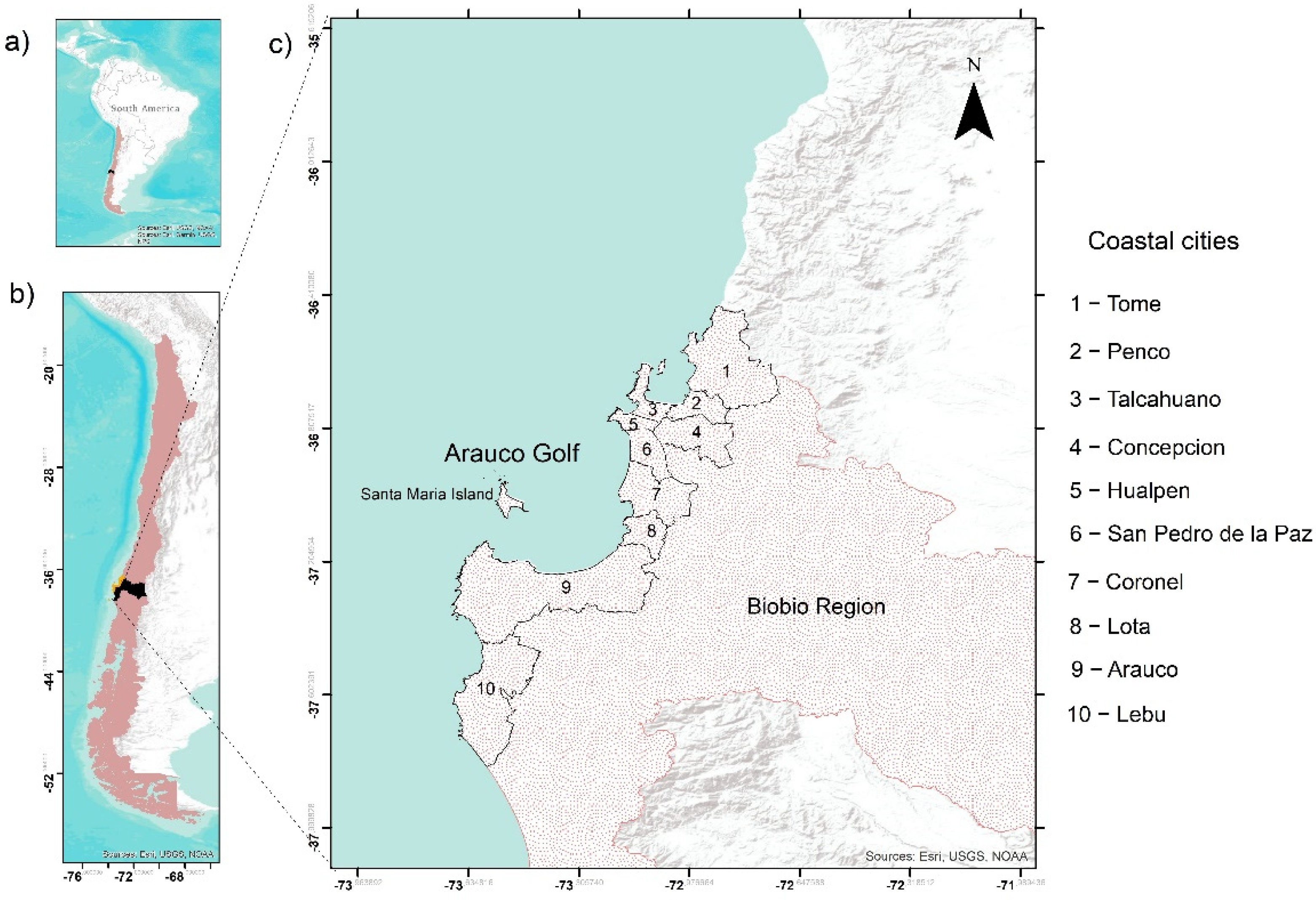
2.1. Study Area

Figure 1a show the location of Chile, which is located in southwestern South America, bordering Peru and Bolivia to the north, Argentina to the east (between the Andes Mountains), and the Pacific Ocean to the west and south. The Biobio region, located in Central Chile and represented in Figure 1b, was one of the most damaged by the 2010 earthquake [25]. The coastal edge of this region is exposed to the latter natural phenomenon, in addition to tsunamis, landslides, and daily seismic activity. Particularly, it was affected by the earthquake and tsunami that impacted small bays along an 800 km stretch of coastline, where 484 people lost their lives. In the Biobio Region, 199 people died, as this area is home to the second-largest conurbation in the country [22,49]. Municipalities of Tome, Penco, Talcahuano, Concepción, Hualpén, San Pedro de la Paz, Coronel, Lota, Arauco, and Lebu are located in the coastal zone of the Biobio region (Figure 1c). These cities represent the second most populated area of the country and play an important role in the region’s economy. In addition, 98% of the exports (not counting copper) use ports located in Central Chile (from latitudes of 33° S to 37° S). Therefore, the identification of surface deformation areas in this area is particularly relevant.

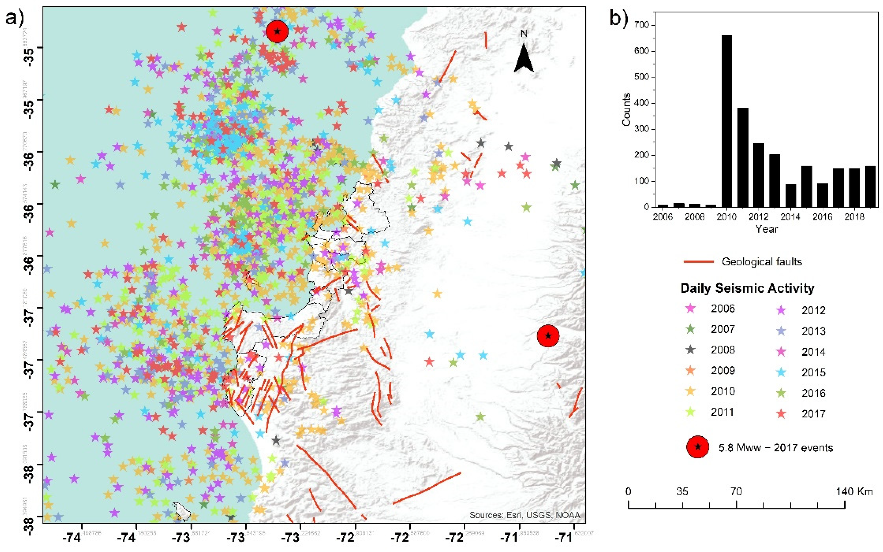
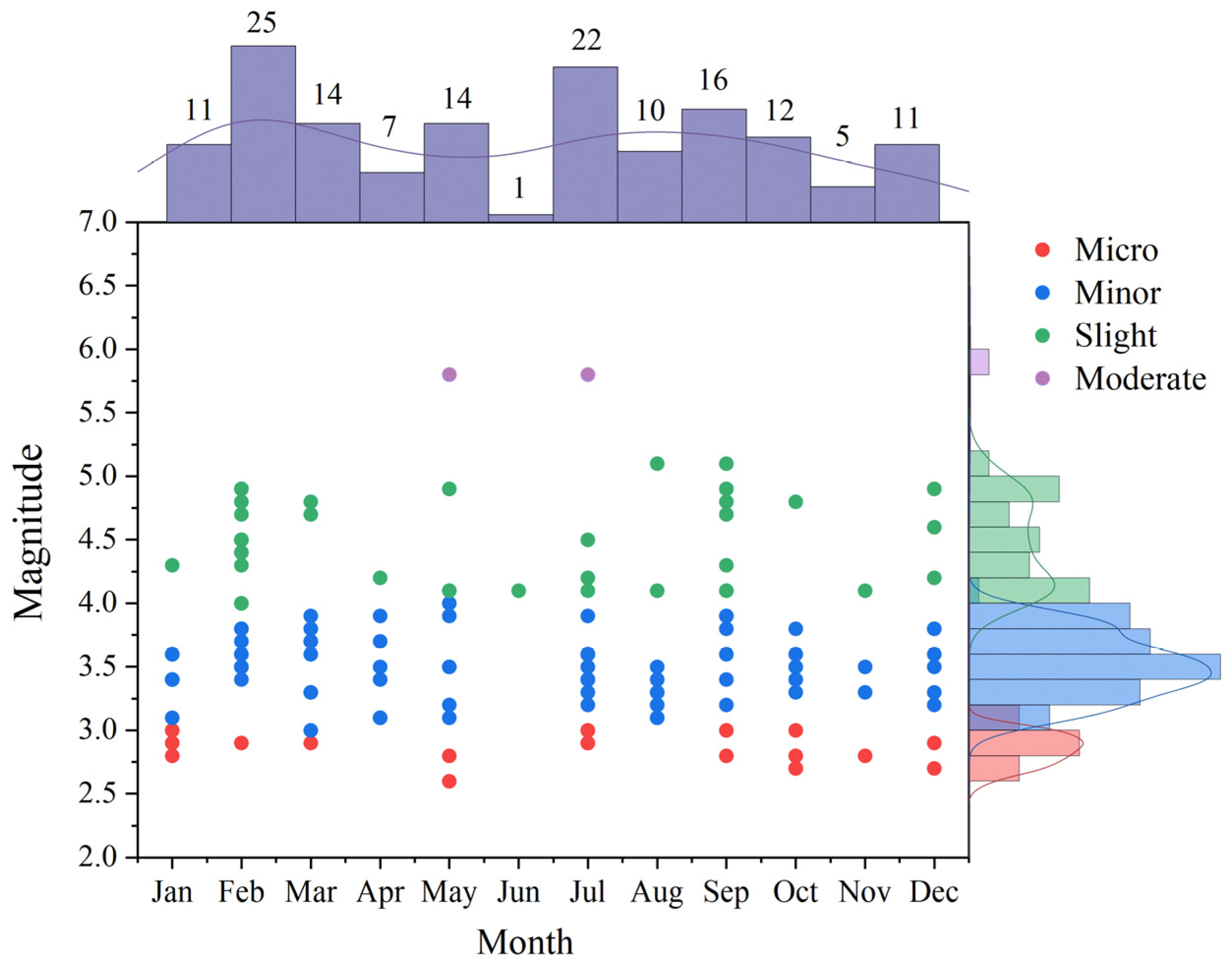
2.2. Classification of Seismic Activity

In seismic countries, there is daily seismic activity, where energy is released over a short or long period. Scientific works are mainly focused on the study of earthquakes that release more energy over a long period [9,18,26,27]. However, this work focused on the study of seismic activity in the range of low to moderate intensity in a short period in the coastal zone of the Biobio region since this energy may be directly related to the risk of deformation in the study area. Earthquakes are classified according to their magnitude and intensity. According to the Seismological Service of the University of Chile [50] (https://www.csn.uchile.cl/, accessed on 17 January 2022), the magnitude measures the energy released in the hypocenter of the earthquake, which is the place where the friction of the plates or their rupture occurs. This is measured with specialized instruments that, where they are located, will register the same magnitude range. Meanwhile, the intensity is not even one; there are several, and we speak of intensities, which objectively measure the violence with which an earthquake is felt at various points in the affected area. Measuring the intensity indicates objectively the violence with which an earthquake is felt at various points in the affected area. The measurement is made by observing the effects or damage produced by the tremor on buildings, objects, the terrain, and the impact it has on people. Its value depends on the distance from the epicenter, type of construction, quality of soil or rock in the locality, and the place where people live [50]. In this work, the United States Geological Survey (USGS) magnitude classification (Richter) was used, as shown in Table 1. For example, a magnitude 5.3 might be computed for a moderate earthquake, and a minor earthquake might be rated as magnitude 3.9. Because of the logarithmic basis of the scale, each whole-number increase in magnitude represents a ten-fold increase in measured amplitude; as an estimate of energy, each whole-number step in the magnitude scale corresponds to the release of about 31 times more energy than the amount associated with the preceding whole-number value. The seismological records around the study area were downloaded from the Centro Sismológico Nacional website (CSN; http://www.sismologia.cl/, accessed on 17 January 2022). The historical recompilation of the daily earthquakes was recorded in the range of 2.0 ≤ M ≤ 5.9 of different magnitude scales covering the time interval from 2006 to 2017. In addition, geological fault data available from SERNAGEOMIN were analyzed (https://www.sernageomin.cl/, accessed on 17 January 2022). The density of low- and medium-intensity earthquakes was estimated using a kernel function in geographical information system (GIS) to fit a smoothly conical surface to the location of each earthquake, using magnitude as the weight [51].
In this study, the local magnitude (Ml) was also used to analyze the intensity of earthquakes. This is determined using the internal waves (primary P waves and secondary S waves) captured by the seismographs of the CSN stations near the place where the earthquake was generated. The W phase (Mww) is also reported, which is a measure of the size of the earthquake and is related to the amount of energy released in the form of elastic waves (internal or surface waves), as well as long-period waves with periods between 200 and 1000 s [50].

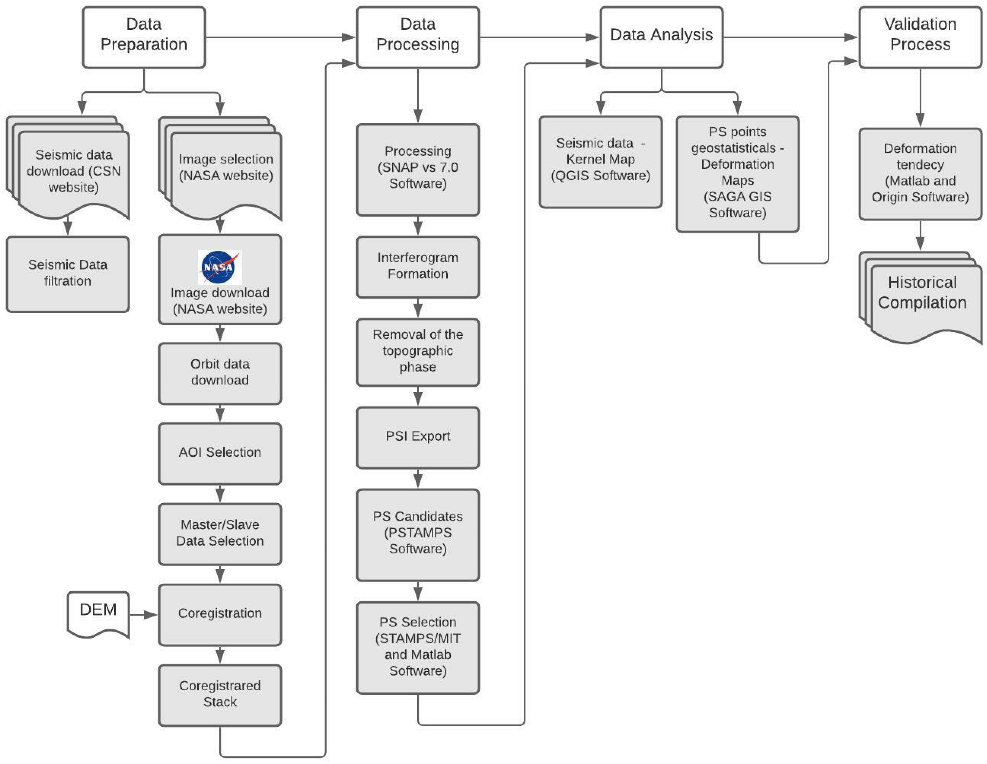
2.3. Data Processing Flow Chart

Figure 2 presents the methodology used for the data processing, which is revealed in four steps. In the data preparation step, the SAR image was selected, downloaded, and pre-processed in SNAP 7.0. Parallel to this, the historical data of earthquakes that occurred in the central region of Chile were downloaded from the CSN. Second, the processing of the images used SNAP and the Stanford method for persistent scatterers (PStaMPS) [52]. Then, to obtain the deformation maps, a spatial statistical analysis was carried out using geographic information systems (QGIS open-source program (https://qgis.org/, accessed on 10 January 2022) and system for automated geoscientific analyses (SAGA) GIS (http://www.saga-gis.org/, accessed on 10 January 2022) using the final PS candidates. Finally, to obtain the trend deformation, the validation process was performed using Matlab 2021 and Origin software (https://www.originlab.com/, accessed on 12 January 2022). Only the Matlab license is required for working with STAMPS/MTI, while the other software mentioned (QGIS, SAGA) could be downloaded freely, thus proving to be cost efficient in comparison to other DInSAR tools, such as Gamma software and SARscape [53]. A more detailed description of each step is provided below.

2.4. Data Preparation and Processing
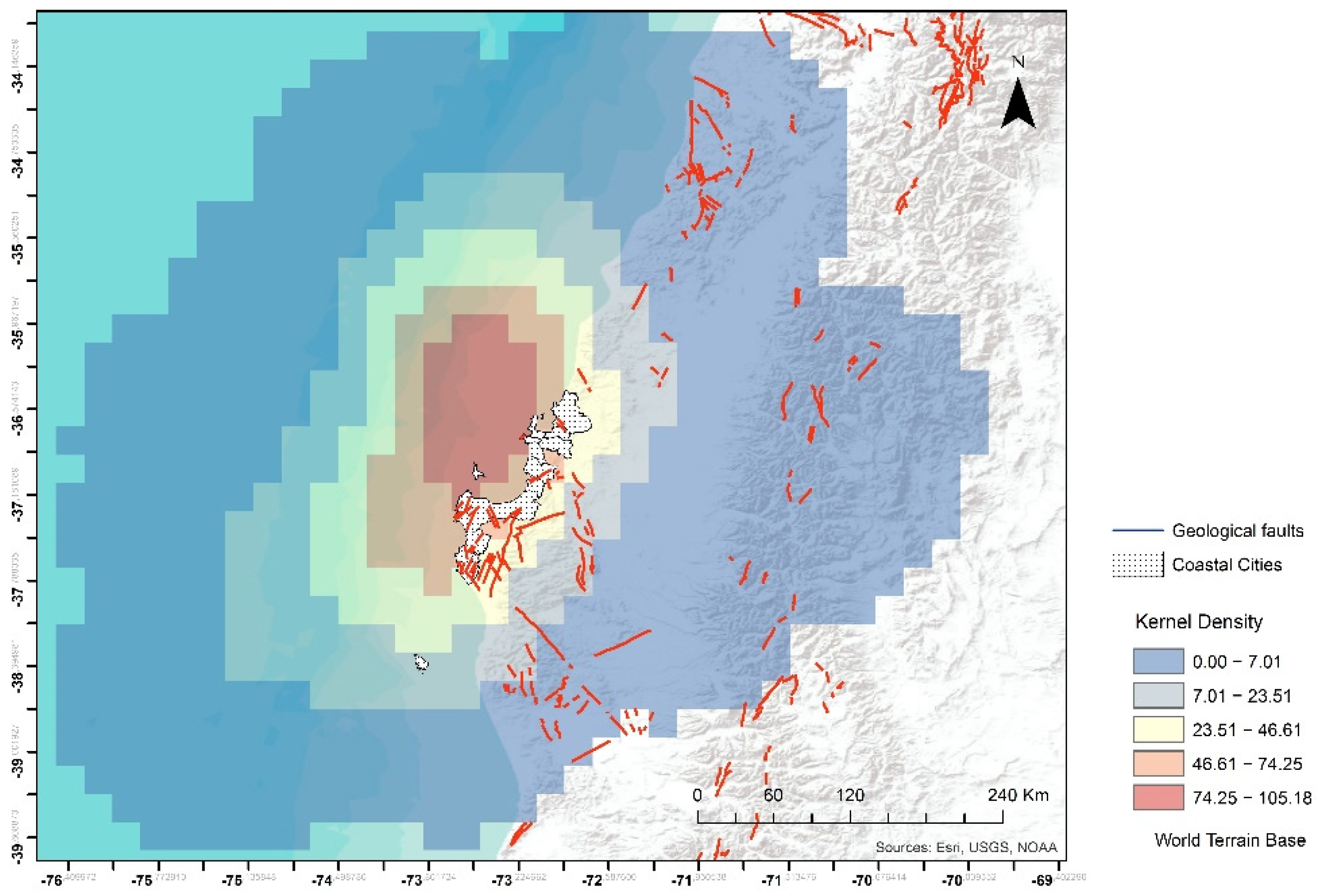
To determine possible changes in the surface of the coastal zone of the Biobio region, a total of 12 raw images from the SENTINEL 1 satellite were selected and downloaded from NASA Earth data (https://search.earthdata.nasa.gov/search/, accessed on 7 January 2022). Ref. [54] showed that using 12 interferograms is usually sufficient when using StaMPS. The year 2017 was chosen for the study area (Figure 1c) because of the quality and availability of images. Information of the radar images selected, sensor, and date of acquisition of the satellite image is shown in Table 2. The pre-process was run in SNAP 7.0 software, where orbit data and digital elevation model (DEM) are downloaded. The images were co-registered using the selected master/slave pairs, and a co-registered stack was obtained [45]. The master image recommended by preprocessing was selected based on the parameters of 2 July 2017 (bperp = 0). Subsequently, 12 interferograms were generated, and the topographic phase was removed and then converted into PS Stamps compatible format (PSI Export). Then, the data were analyzed with the persistent scatterer (PS) method [46]. In total, 1,334,951 PS points were selected from 5,947,735 PS candidates, representing points where deformation can be monitored. The PS points distributed over the extension of the study area are represented in deformation velocity maps. The line-of-sight (LOS) represents the measurement of the deformation rate; in other words, it indicates that there was a decrease or increase in the area, based on the geometry of the sensor based on the slant range or across-track direction [55]. Then the PS candidates were processed in StaMPS/MIT [52] software version 4.1b, Linux environment, to select the final PS candidates.
The interferometric wide-swath (IW) mode of operation was used, which is the one set to perform interferometric and descending orbit processing. To generate quality interferograms, VV polarizations were used, due to their vertical representativeness following the approach of [56], with a range length of 250 km with resolutions of 5 × 20 m in range and azimuth, respectively. Single look complex (SLC) has 3 subframes (Subwaths IW1, IW2, and IW3), and IW1 was used for the chosen area.

2.5. Data Analysis

The deformation is defined as the surface variation of the investigated area. To reduce the effect of spatial decorrelation and errors induced by DEM inaccuracy, only interferograms with small orbital baselines were selected for subsequent time-series analyses. This method is based on the phase comparison of multiple SAR images gathered at different times over the study region and allows for measurements of land deformation along the LOS direction of the SAR sensor with up to millimeter precision [57]. In addition, a procedure is implemented to reduce the de-correlation effect caused by noise and avoid its negative impact when calculating the LOS offset. PS are artificial objects that reflect the radar signal well, such as metal structures, buildings, and rock outcrops, and are used in persistent scatterer interferometry (PSI), e.g., the permanent scatterers (PS-InSAR) technique [28,40]. In urban areas, there is a prevalence of PS, and PSI methods allow for the analysis of even individual structures on the ground. PS can be geolocated more accurately, and a residual error of the residual DEM can be calculated after the initial subtraction of the DEM. Various types of PS can be distinguished from each other, and provide a way to locate points in the resolution cell [28,58]. This type of processing reduces the atmospheric noise generated by conventional processing [46,47]. Then, all PS points were generated following the method proposed in [52]. The vertical displacement (vd) was calculated in the following Equation (1).
vd = −LOS × 1/cosθ
where LOS is the unwrapped phase obtained by InSAR processing and θ = 37.32 is the incidence angle [59].
From the data analysis, it was possible to generate 12 deformation maps (a map by month) in the study area for the year 2017. All maps were created via the universal Kriging method [60,61] in SAGA GIS 2.3.2 software [62].

2.6. Validation Process

To identify the areas with the greatest deformation within the coastal edge, a trend map was generated using Matlab 2021. The trend map was constructed by estimating the linear trend of the InSAR time series for each pixel, using least-squares fitting. For the trend analysis, the 12-month LOS values were considered and interpolated in SAGA GIS 2.3.2, generating a map with deformation trend information. A second graph was generated through Origin software to identify spatial trend patterns of deformation as a function of latitude and longitude. Through the historical recompilation, it was possible to corroborate with the trend map and the directions in which the uplift movements are mainly generated. Previous studies demonstrated by geodesic studies and environmental indicators where the cities of Arauco and Lebu are moving [63,64].

3. Results and Discussion

3.1. Low/Medium Intensity Seismic Range

Figure 3a shows the relevant seismic activity in the study area during the 2006–2017 years. Considering this period, the area has several 2023 daily earthquakes. Seismic activity is concentrated offshore. It is important to note that the area that shows the highest concentration of earthquakes is close to geological faults, for example, in the Arauco peninsula. The highest percentage of earthquakes had magnitudes between 2.0 and 4.9 with 93.03% in total on the Richter scale. Magnitudes between 5.0 and 5.9 (moderate) occurred in 6.18%, while those greater than 5.9 (strong) on the Richter scale occurred in 0.79% of the cases. Therefore, it is possible to suggest that the studied area is characterized by seismic events of micro, minor, and slight magnitude. The highest seismicity was found in 2010 and was due to the 27F event (Mw 8.8) (Figure 3b).
Figure 4 shows the hot spot patterns of earthquake occurrence based on kernel density analysis. The complete data set (Figure 4) showed the presence of a large cluster offshore of Concepcion Bay; however, it is also possible to observe that all cities that make up the study area are located within the zone with the highest and very highest density of daily earthquakes, represented by orange and red colors.
Although the north of the country was identified with a higher concentration of earthquakes with magnitudes greater than 5.0 Richter in the last 10 years, specifically in the coastal area of the Tarapacá region and in the high plateau area of the Antofagasta region [65], the central zone of Chile, between 30° S and 35° S, is a very active seismic zone with a great diversity of subduction earthquakes and has evidenced the most catastrophic events occurring in the country and the world. Therefore, a priority task today is to develop Chile’s capabilities and competencies for the study of earthquakes, using new technologies and signals obtained from satellites/radar and GIS.
Figure 5 shows a monthly distribution of seismic events classified by magnitude during the year 2017. It also shows the distribution of magnitude frequency classified according to Table 1. Particularly, for the year 2017, a total of 148 daily earthquakes were recorded (taking as references the cities investigated), with magnitudes from 2.7 Ml to 5.8 Mww. Evaluating this period, February was identified as the month with the highest number of earthquakes, registering a total of 25 daily earthquakes. June has the lowest number with 1 earthquake for the entire period. When looking at the magnitudes, it is possible to perceive that all months, except June, presented micro, minor, slight, and moderate earthquakes. The months with the highest seismological magnitude (5.8) were May and July (showed in red circles in Figure 3). Thus, we can say that the period was characterized by events with magnitudes between 3 and 4, classified as being of minor intensity.

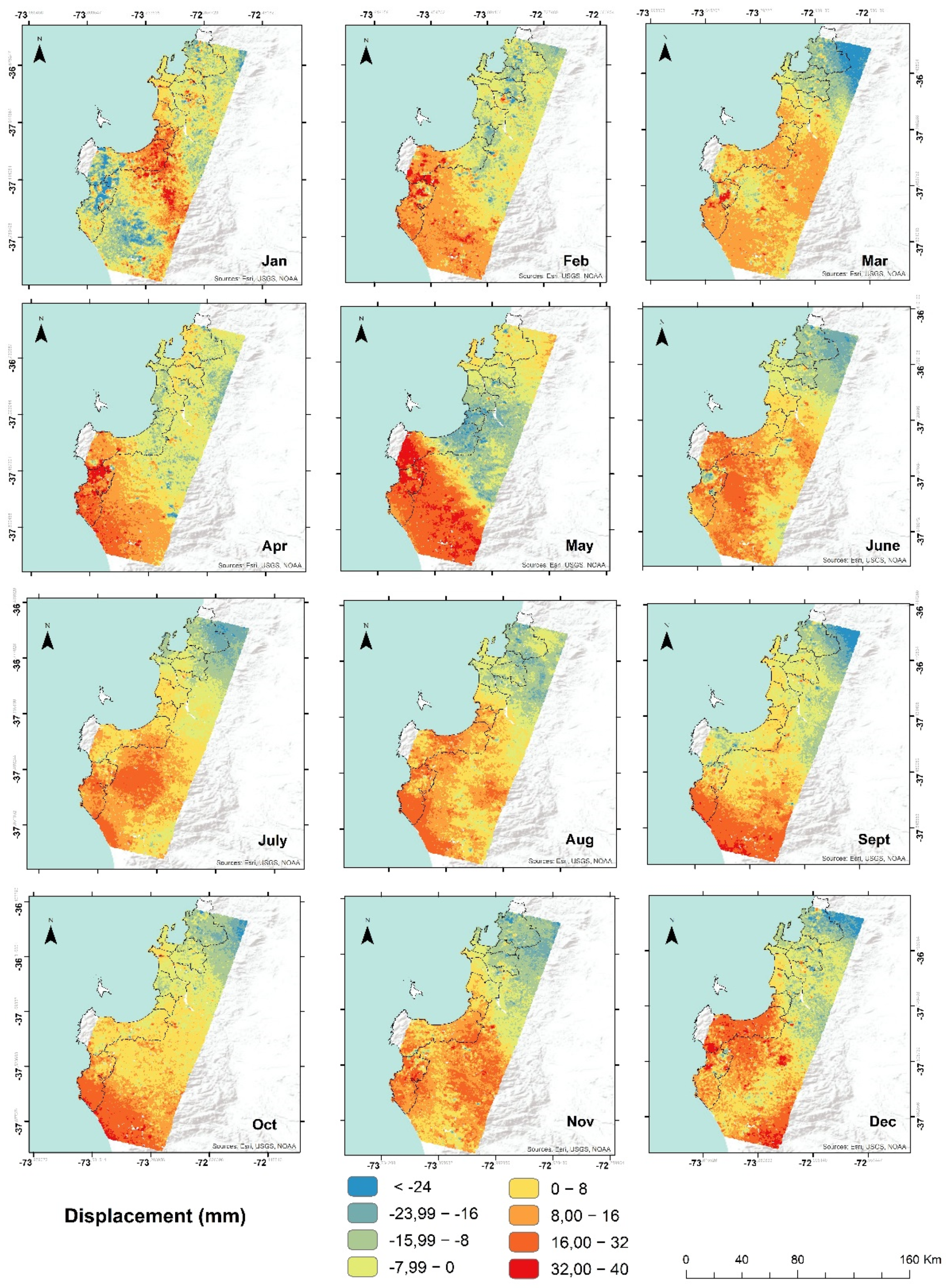
3.2. Deformation Maps

Seismic activity in the coastal zone of the Biobio region is a recurrent phenomenon, but to our knowledge, it is not known if it is the main cause of deformation in the area. In this research, deformation was identified to establish its relationship with the seismic component in the coast of the Biobio region. The total displacement field estimated by PSI for the period spanning from January to December 2017 is displayed in Figure 6. The colored pixels represent those scatterers interpolated that are found to be coherent and selected as PS. To reduce the influence of a single scatterer, we average the displacements of the PS inside this area. After the phase noise estimate, the overall noise was reduced, and PS points filtered. Several stable-phase pixels are 1,334,951. Weed standard deviation = 1, and bad PS pixels (too much noise or ground contributions). The ‘Unwrapprefilter_flag’ parameter was kept in ‘y’ to improve the accuracy of the unwrapping. Positive values indicate that the deformation approached the satellite in the direction of the line-of-sight (LOS); negative values denote that deformation in the LOS motion turned aside, away from the satellite. The monthly maps show the uplift and subsidence in the area, represented by red and blue colors, respectively, with a pixel of 0.2°. The month of May registered the highest range of displacement for the area with values of 40 mm and −24 mm. On the other hand, July presented values between 24 mm and −16 mm. It is important to note that both months have a maximum magnitude of 5.8 Mww recorded. Comparing the location between the two epicenters (Figure 3), the earthquake referring to the month of May is located in the continent (−37.345° S, −71.783° W,) and the earthquake referring to the month of July is located in the sea (−37.345° S, −73.361° W) [50]. The seismic wave has different behaviors depending on the propagation material, and water wave propagation in ocean seismology still represents a challenge for researchers [66]. Geology and soil types (solid materials) are factors to be considered during the investigation of seismic wave propagation [67]. Another reason why July may not show such a high displacement range when compared to May is that this month’s image was used as a master during processing. In addition, it is observed that during 7 months of the year, there are values of −24 mm.
It can be observed in Figure 6 the distribution of magnitudes of the earthquakes recorded for 2017, by month. It also shows the distribution of the monthly quantity and magnitudes frequency, classified according to Table 1. February is the month with the highest monthly number, registering a total of 25 daily earthquakes, and June has the lowest number with 1 earthquake for the entire month. When looking at the magnitudes, it is possible to perceive that all months, except June, presented micro, minor, slight, and moderate earthquakes. The highest frequency of earthquakes is between 3.0 Mw and 4.0 Mw, and then between 4.0 Mw and 5.0 Mw. May and July showed the highest magnitudes when compared to the other months. Evaluating the deformation data, it is possible to perceive that May presents the highest value of positive deformation (40 mm), and November has the lowest value (20 mm). December has the highest negative maximum. July, August, and October have the lowest negative maxima. January and May have deformation ranges (0 mm and 16 mm, respectively) different from the other months that remained constants (8 mm). Another reason why July may not show such a high displacement range when compared to May is that this month’s image was used as a master during processing. In other words, to determine the differential values, July was taken as the base month concerning the other months.

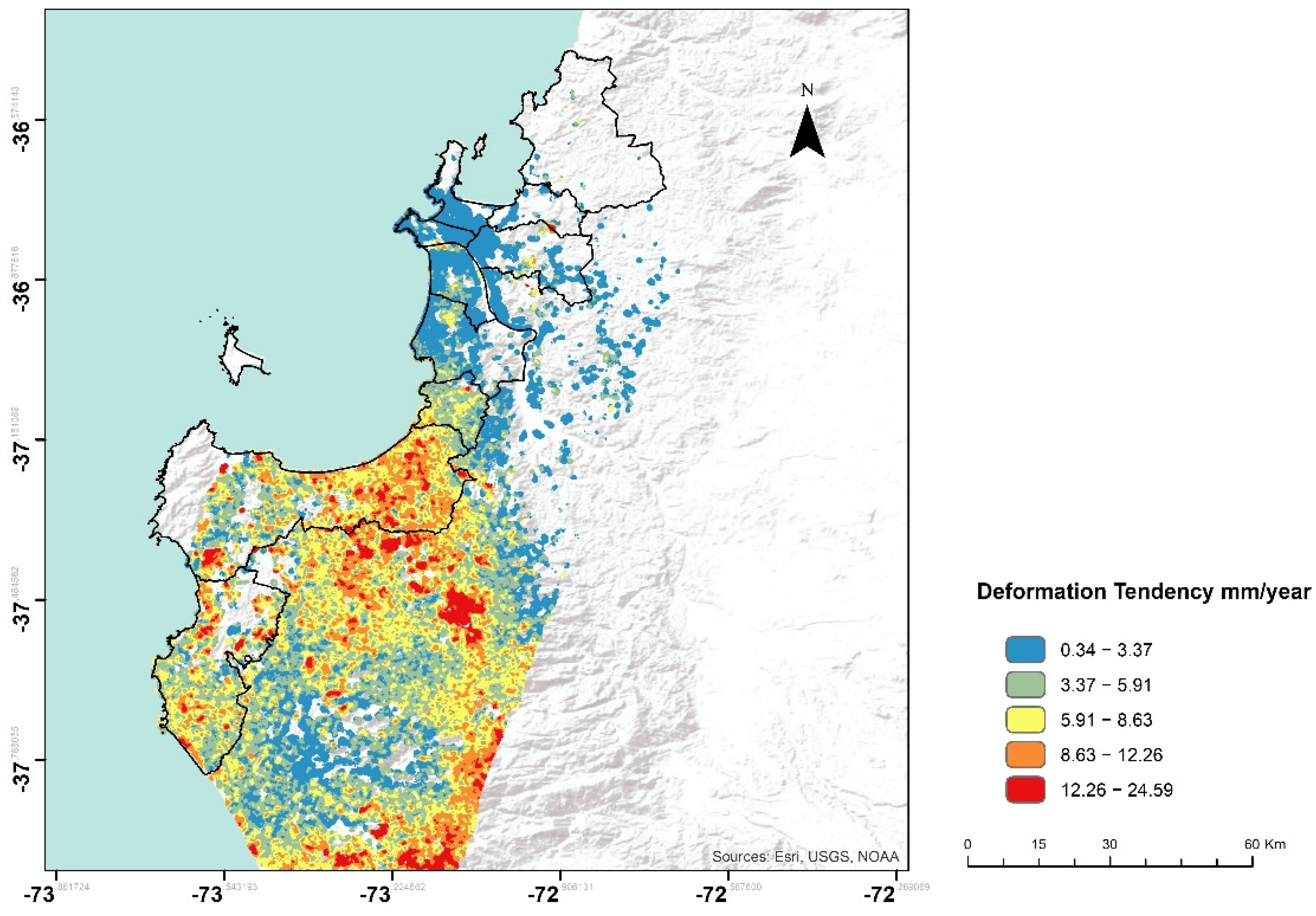
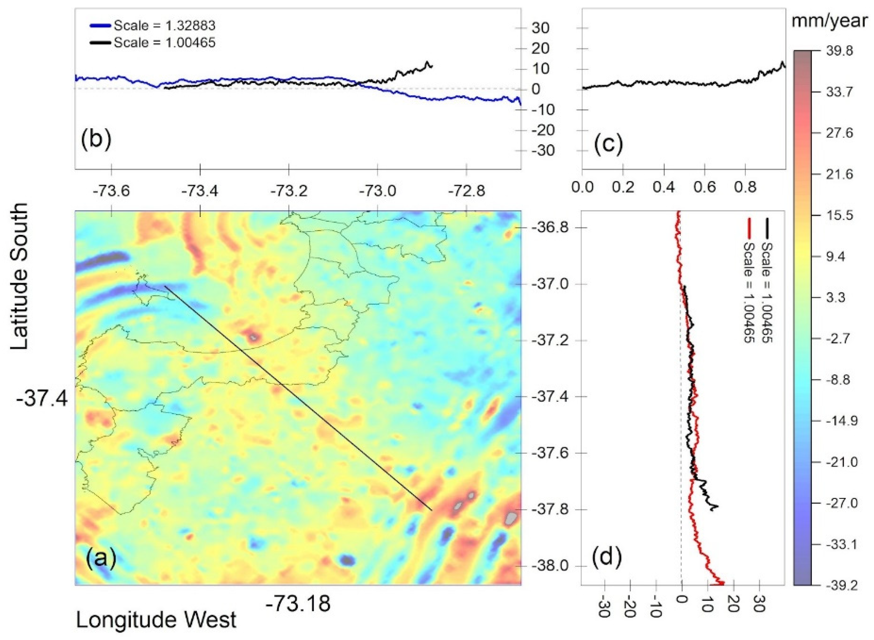
3.3. Trend Deformation Maps

Figure 7 represents the linear trend map interpolated from the Kriging method. Based on the trend map, it can be observed that the coastal presented a slight upward trend in the north and northeast zone (i.e., δup ~3 mm/year), in blue color. However, in the south and southwest zone, in the case of transverse monitoring of Arauco Bay, it presented a more accentuated upward trend (i.e., δup ~24 mm/year), in red color. In addition, a clear deformation pattern is defined along the coast, being greater in the Gulf of Arauco, and Lebu. One study reports [68] the rate of ± 1.5 mm/year as the stable zone threshold. In this sense, a rate above this threshold is significant for a possible landslide event or other associated hazards. This trend map already indicates which zones are susceptible to deformation, either in the form of uplift or subsidence. This result related to the identification of risk areas is consistent with the report previously by Ref. [65].
Figure 8 shows the spatial patterns of the deformation for the selected study areas. Studying the entire displacement field depicted in Figure 8a, we observe a slight uplift trend up to longitude 73.0, wherefrom this point, the terrain tends to dip (approximately about −10 mm/year) (Figure 8b). In Figure 8c, the graph represents the cross section to Arauco Bay, where there is a slight elevation trend. Figure 8d shows that at higher latitudes, starting from latitude 37.0 in a southerly direction, the terrain begins to rise. Figure 8a shows that of the municipalities studied, Lota, Arauco, and Lebu have the greatest tendencies to rise when compared to the other municipalities located further north in this study. This pattern is related to the daily seismic activity (see Figure 3), the product of the movement between plates, and the geological faults located in the area.
This trend behavior was verified previously by [12,63,64], which demonstrated the effects of the co-seismic uplift in four peninsulas that make up the region studied, after the 27F earthquake. The retreat of the sea was observed on some beaches, and the dehydration of the Raqui-Tubul wetland in Arauco [69], and the drying up of the Lebu River [63]. Santa Maria island, located in the Arauco Gulf, shows subsidence and uplift tendency patterns in some areas, between −14.9 and 39.2 mm/year (Figure 8a). The coastal subsidence trend was also identified by [14], who conducted a study where they recorded that the small island underwent elevation changes between co-seismic cycles between the 1835 and 2010 earthquakes. Therefore, the deformation and tendency maps provide certainty in terms of where hotspots are located, e.g., the most hazardous areas in the study zone.
Slopes under seismic excitation are one of the most important problems to consider [70]. In the study area, it was verified in works by [63,64] that the seismic movements that occurred can generate changes in the relief. These changes occurred under large seismic energy releases. However, it can be observed with the data presented in this study that deformation can also be identified in periods with earthquakes of lower to moderate intensities by using radar techniques. This fact opens a space for future research on potential hazards related to slope stability in areas with potential and active landslides recorded in the study area. Inspired by two studies cited by [55], it was reported that they were intended to model the post seismic displacement that continued to occur at the site after the earthquake. Interferometry played an important role in this study since most of these displacements were aseismic, and therefore went unnoticed by conventional seismological records. Based on their results, it is clear that to capture the smallest displacement structures with ground-based instrumentation, such as GPS receivers, it would be necessary to cover the ground with instruments and that such a density is not realistic.
Some limitations faced by this study are the limited period of investigation, the computational resources (e.g., clusters), the corroboration of the processed data with in situ data, and analyses with other seismic indicators (such as acceleration). Therefore, future research should include GPS/GNSS data time series, shear wave propagation velocity in the surface 30 m (Vs30) and seismic microzonation [29] as an index to characterize the seismic amplification of the ground and thus classify sites with different seismic demand, and record landslides in the area to improve our understanding of potential hazards.

4. Conclusions

Due to the advances in technologies applied to geosciences, the InSAR method has gained an important role in research in the field of earthquake deformations. Therefore, we presented a spatial–temporal distribution of deformations and trends of deformation during the 2017 year, which was derived from 12 Sentinel-1B images using the InSAR method. On the other hand, the seismic activity was analyzed, and the geoinformation obtained from the InSAR analysis was corroborated with the daily seismic records. Based on the results, the following was found:
(1) The central coast of Chile is characterized by seismic events of micro, minor, and slight magnitudes with a prevalence of 93.03% for the study period. Based on kernel analysis, the coastal zone is identified as having a high density of daily earthquakes, located from the bay of Arauco to the ocean.
(2) Monthly deformation maps were developed for 10 municipalities on the coast of the Biobio region in Central Chile. The data corroborated with daily earthquakes and proximity to fault zones show deformation for all months, highlighting the month of May, with the highest range of displacement (40 and −24 mm/year). July also recorded the same seismic magnitude, but the range of displacement is smaller than May month, which may be related to the location of the epicenter offshore or the radar perception.
(3) The coastal zone presented a slight upward deformation tendency in the north and northeast zone (i.e., δup ~3 mm/year), while the south and southwest zone presented a more accentuated upward trend (i.e., δup ~24 mm/year). The municipalities of Lota, Arauco, and Lebu have a greater tendency of deformation.
Future research will include more radar images with an extension of the analysis period and at the same time corroborate with other techniques, such as the GNSS.

Author Contributions

Conceptualization, L.d.D.d.J.d.S., L.R.-L., L.G.-R., H.M.C. and M.I.A.A.; methodology, L.d.D.d.J.d.S.; software, L.d.D.d.J.d.S., L.M.C.S., H.M.C. and L.G.-R.; validation, L.d.D.d.J.d.S.; formal analysis, L.d.D.d.J.d.S. and M.I.A.A.; investigation, L.d.D.d.J.d.S. and M.I.A.A.; resources, M.I.A.A.; data curation, L.d.D.d.J.d.S., M.I.A.A. and H.M.C.; writing—original draft preparation, L.d.D.d.J.d.S., L.R.-L. and L.G.-R.; writing—review and editing, M.I.A.A. and H.M.C.; visualization, M.I.A.A.; supervision, M.I.A.A.; project administration, M.I.A.A. All authors have read and agreed to the published version of the manuscript.

Funding

This research was funded by Universidad de Concepción, Chile.

Institutional Review Board Statement

Not applicable.

Informed Consent Statement

Not applicable.

Data Availability Statement

Not applicable.

Acknowledgments

The authors thank the Kultrum Project-Astronomy Department and Urban Planning Department from the University of Concepcion, Chile to support this research. L.R.-L. thanks to project VRIDFAI21/10 of the Universidad San Sebastian and to the CRHIAM Water Center (Project ANID/FONDAP/15130015).

Conflicts of Interest

The authors declare no conflict of interest.

References

  1. Spieker, K.; Rondenay, S.; Sawade, L. Long-range Receiver Function Profile of Crustal and Mantle Discontinuities from the Aleutian Arc to Tierra del Fuego. Geophys. Res. Abstr. 2016, 18, 9120. [Google Scholar]
  2. Berz, G.; Kron, W.; Loster, T.; Rauch, E.; Schimetschek, J.; Schmieder, J.; Siebert, A.; Smolka, A.; Wirtz, A. World map of natural hazards—a global view of the distribution and intensity of significant exposures. Nat. Hazards 2001, 23, 443–465. [Google Scholar] [CrossRef]
  3. Sidorin, A.Y. A Look at the 1988 Spitak Earthquake in the Light of Lessons Learned from the 1948 Ashgabat Catastrophe. Izv.-Atmos. Ocean Phys. 2019, 55, 1774–1786. [Google Scholar] [CrossRef]
  4. Sepúlveda, M.E.P.-B. La gestión de una catástrofe a principios del siglo XX: El terremoto de 1906 en Valparaíso (Chile). Antíteses 2021, 14, 344. [Google Scholar] [CrossRef]
  5. Lemenkova, P. Visualization of the geophysical settingsin the Philippine Sea margins by means of GMT and ISC data. Cent. Eur. J. Geogr. Sustain. Dev. 2020, 2, 5–15. [Google Scholar] [CrossRef]
  6. Lin, X. Risk awareness and adverse selection in catastrophe insurance: Evidence from California’s residential earthquake insurance market. J. Risk Uncertain. 2020, 61, 43–65. [Google Scholar] [CrossRef]
  7. Eslamian, S.; Eslamian, F.; Frameworks, N.; Resilience, B. Handbook of Disaster Risk Reduction for Resilience; Springer: Cham, Switzerland, 2021; ISBN 9783030612771. [Google Scholar]
  8. De la Llera, J.C.; Rivera, F.; Mitrani-Reiser, J.; Jünemann, R.; Fortuño, C.; Ríos, M.; Hube, M.; Santa María, H.; Cienfuegos, R. Data Collection after the 2010 Maule Earthquake in Chile; Springer: Cham, Switzerland, 2017; Volume 15, ISBN 1051801699183. [Google Scholar]
  9. Castilla, J.C.; Manríquez, P.H.; Camaño, A. Effects of rocky shore coseismic uplift and the 2010 Chilean mega-earthquake on intertidal biomarker species. Mar. Ecol. Prog. Ser. 2010, 418, 17–23. [Google Scholar] [CrossRef] [Green Version]
  10. Jiménez Martínez, M.; Jiménez Martínez, M.; Romero-Jarén, R. How Resilient is the Labour Market against Natural Disaster? Evaluating the Effects from the 2010 Earthquake in Chile; Springer: Cham, Switzerland, 2020; Volume 104, ISBN 0123456789. [Google Scholar]
  11. Lagos López, M.; Cisternas Vega, M. El nuevo riesgo de tsunami: Considerando el peor escenario. Scr. Nova Rev. Electron. Geogr. y Ciencias Soc. 2008, 12, 25. [Google Scholar] [CrossRef]
  12. Vargas, G.; Farías, M.; Carretier, S.; Tassara, A.; Baize, S.; Melnick, D. Coastal uplift and tsunami effects associated to the 2010 Mw8.8 Maule earthquake in central Chile. Andean Geol. 2011, 38, 219–238. [Google Scholar] [CrossRef] [Green Version]
  13. Flores, M.; Hern, J.R. Procesos de remoción en masa inducidos por el terremoto del 27F de 2010 en la franja costera de la Región del Biobío, Chile. Rev. Geogr. Norte Gd. 2012, 74, 57–74. [Google Scholar] [CrossRef] [Green Version]
  14. Wesson, R.L.; Melnick, D.; Cisternas, M.; Moreno, M.; Ely, L.L. Vertical deformation through a complete seismic cycle at Isla Santa María, Chile. Nat. Geosci. 2015, 8, 547–551. [Google Scholar] [CrossRef]
  15. Lapere, R.; Mailler, S.; Menut, L. The 2017 mega-fires in central chile: Impacts on regional atmospheric composition and meteorology assessed from satellite data and chemistry-transport modeling. Atmosphere 2021, 12, 344. [Google Scholar] [CrossRef]
  16. Van Eaton, A.R.; Amigo, Á.; Bertin, D.; Mastin, L.G.; Giacosa, R.E.; González, J.; Valderrama, O.; Fontijn, K.; Behnke, S.A. Volcanic lightning and plume behavior reveal evolving hazards during the April 2015 eruption of Calbuco volcano, Chile. Geophys. Res. Lett. 2016, 43, 3563–3571. [Google Scholar] [CrossRef] [Green Version]
  17. Gironás, J.; Bunster, T.; Chadwick, C.; Fernández, B. Floods. In Water Resources of Chile; Fernández, B., Gironás, J., Eds.; Springer: Berna, Switzerland, 2021; Volume 8, ISBN 978-3-030-56901-3. [Google Scholar]
  18. Ruiz, S.; Madariaga, R. Historical and recent large megathrust earthquakes in Chile. Tectonophysics 2018, 733, 37–56. [Google Scholar] [CrossRef]
  19. Daniell, J.E.; Schaefer, A.M.; Wenzel, F. Losses associated with secondary effects in earthquakes. Front. Built Environ. 2017, 3, 30. [Google Scholar] [CrossRef]
  20. Wang, T.; DeGrandpre, K.; Lu, Z.; Freymueller, J.T. Complex surface deformation of Akutan volcano, Alaska revealed from InSAR time series. Int. J. Appl. Earth Obs. Geoinf. 2018, 64, 171–180. [Google Scholar] [CrossRef]
  21. Khan, G.; Qureshi, J.A.; Khan, A.; Shah, A.; Ali, S.; Bano, I.; Alam, M. The role of sense of place, risk perception, and level of disaster preparedness in disaster vulnerable mountainous areas of Gilgit-Baltistan, Pakistan. Environ. Sci. Pollut. Res. 2020, 27, 44342–44354. [Google Scholar] [CrossRef] [PubMed]
  22. Bresciani Lecannelier, L.E. De la Emergencia a la Política de Gestión de Desastres: La Urgencia de Institucionalidad Pública para la Reconstrucción; C.I.P.–Pontificia Universidad Católica de Chile, Centro de Politicas Publicas: Santiago, Chile, 2012; ISBN 9789561413115. [Google Scholar]
  23. Piersanti, A.; Spada, G.; Sabadini, R.; Bonafede, M. Global post-seismic deformation. Geophys. J. Int. 1995, 120, 544–566. [Google Scholar] [CrossRef] [Green Version]
  24. Valerio, E.; Tizzani, P.; Carminati, E.; Doglioni, C.; Pepe, S.; Petricca, P.; De Luca, C.; Bignami, C.; Solaro, G.; Castaldo, R.; et al. Ground deformation and source geometry of the 30 October 2016M w 6.5 norcia earthquake (Central Italy) investigated through seismological data, DInSAR measurements, and numerical modelling. Remote Sens. 2018, 10, 1901. [Google Scholar] [CrossRef] [Green Version]
  25. Kovacs, P. Reducing the Risk of Earthquake Damage in Canada: Lessons from Haiti and Chile; The Institute for Catastrophic Loss Reduction: Toronto, ON, Canada, 2010; ISBN 9780978484163. [Google Scholar]
  26. Tamkuan, N.; Nagai, M. Sentinel-1a Analysis for Damage Assessment: A Case Study of Kumamoto Earthquake in 2016. MATTER Int. J. Sci. Technol. 2019, 5, 23–35. [Google Scholar] [CrossRef] [Green Version]
  27. Suresh, D.; Yarrakula, K. InSAR based deformation mapping of earthquake using Sentinel 1A imagery. Geocarto Int. 2020, 35, 559–568. [Google Scholar] [CrossRef]
  28. Ferretti, A.; Prati, C.; Rocca, F. Permanent scatterers in SAR interferometry. IEEE Trans. Geosci. Remote Sens. 2001, 39, 8–20. [Google Scholar] [CrossRef]
  29. Gatto, M.P.A.; Montrasio, L.; Zavatto, L. Experimental Analysis and Theoretical Modelling of Polyurethane Effects on 1D Wave Propagation through Sand-Polyurethane Specimens. J. Earthq. Eng. 2021, 25, 1–25. [Google Scholar] [CrossRef]
  30. Gatto, M.P.A.; Montrasio, L.; Berardengo, M.; Vanali, M. Experimental Analysis of the Effects of a Polyurethane Foam on Geotechnical Seismic Isolation. J. Earthq. Eng. 2020, 24, 1–22. [Google Scholar] [CrossRef]
  31. Gatto, M.P.A.; Lentini, V.; Castelli, F.; Montrasio, L.; Grassi, D. The use of polyurethane injection as a geotechnical seismic isolation method in large-scale applications: A numerical study. Geosciences 2021, 11, 201. [Google Scholar] [CrossRef]
  32. Pamukçu, O.; Gönenç, T.; Çirmik, A.; Sindırgi, P.; Kaftan, İ.; Akdemir, Ö. Investigation of vertical mass changes in the south of Izmir (Turkey) by monitoring microgravity and GPS/GNSS methods. J. Earth Syst. Sci. 2015, 124, 137–148. [Google Scholar] [CrossRef]
  33. Gatsios, T.; Cigna, F.; Tapete, D.; Sakkas, V.; Pavlou, K.; Parcharidis, I. Copernicus sentinel-1 MT-InSAR, GNSS and seismic monitoring of deformation patterns and trends at the methana volcano, Greece. Appl. Sci. 2020, 10, 6445. [Google Scholar] [CrossRef]
  34. Pritchard, M.E. InSAR, a tool for measuring Earth’s surface deformation. Phys. Today 2006, 59, 68–69. [Google Scholar] [CrossRef] [Green Version]
  35. Dwivedi, R.; Narayan, A.B.; Tiwari, A.; Dikshit, O.; Singh, A.K. Multi-temporal SAR Interferometry for landslide monitoring. Int. Arch. Photogramm. Remote Sens. Spat. Inf. Sci.-ISPRS Arch. 2016, 41, 55–58. [Google Scholar] [CrossRef] [Green Version]
  36. Jo, M.J.; Jung, H.S.; Yun, S.H. Retrieving Precise Three-Dimensional Deformation on the 2014 M6.0 South Napa Earthquake by Joint Inversion of Multi-Sensor SAR. Sci. Rep. 2017, 7, 5485. [Google Scholar] [CrossRef] [Green Version]
  37. Yang, C.; Han, B.; Zhao, C.; Du, J.; Zhang, D.; Zhu, S. Co- and post-seismic deformation mechanisms of the MW 7.3 Iran earthquake (2017) revealed by Sentinel-1 InSAR observations. Remote Sens. 2019, 11, 418. [Google Scholar] [CrossRef] [Green Version]
  38. Peng, M.; Lu, Z.; Zhao, C.; Motagh, M.; Bai, L.; Conway, B.D.; Chen, H. Mapping land subsidence and aquifer system properties of the Willcox Basin, Arizona, from InSAR observations and independent component analysis. Remote Sens. Environ. 2022, 271, 112894. [Google Scholar] [CrossRef]
  39. Alves, N.L.; Galo, M.; Galo, M.L.B.T. Fundamentos do processamento interferométrico de dados de radar de abertura sintética. In Proceedings of the Anais XIV Simpósio Brasileiro de Sensoriamento Remoto, Natal, Brazil, 25–30 April 2009; pp. 7227–7234. [Google Scholar]
  40. Ferretti, A.; Prati, C.; Rocca, F. Nonlinear subsidence rate estimation using permanent scatterers in differential SAR interferometry. IEEE Trans. Geosci. Remote Sens. 2000, 38, 2202–2212. [Google Scholar] [CrossRef] [Green Version]
  41. Huang, Q.-H.; He, X.-F. Surface deformation investigated with SBAS-DInSAR approach based on prior knowledge. Remote Sens. Spat. Inf. Sci. 2008, 37, 99–104. [Google Scholar]
  42. Bianchini, S.; Ciampalini, A.; Raspini, F.; Bardi, F.; Di Traglia, F.; Moretti, S.; Casagli, N. Multi-Temporal Evaluation of Landslide Movements and Impacts on Buildings in San Fratello (Italy) By Means of C-Band and X-Band PSI Data. Pure Appl. Geophys. 2015, 172, 3043–3065. [Google Scholar] [CrossRef] [Green Version]
  43. Orellana, F.; Blasco, J.M.D.; Foumelis, M.; D’aranno, P.J.V.; Marsella, M.A.; Mascio, P. Di Dinsar for road infrastructure monitoring: Case study highway network of Rome metropolitan (Italy). Remote Sens. 2020, 12, 3697. [Google Scholar] [CrossRef]
  44. Ferretti, A.; Fumagalli, A.; Novali, F.; Prati, C.; Rocca, F.; Rucci, A. A new algorithm for processing interferometric data-stacks: SqueeSAR. IEEE Trans. Geosci. Remote Sens. 2011, 49, 3460–3470. [Google Scholar] [CrossRef]
  45. Cavur, M.; Moraga, J.; Sebnem Duzgun, H.; Soydan, H.; Jin, G. Displacement analysis of geothermal field based on psinsar and som clustering algorithms: A case study of Brady field, Nevada—USA. Remote Sens. 2021, 13, 349. [Google Scholar] [CrossRef]
  46. Hooper, A.; Zebker, H.; Segall, P.; Kampes, B. A new method for measuring deformation on volcanoes and other natural terrains using InSAR persistent scatterers. Geophys. Res. Lett. 2004, 31, 1–5. [Google Scholar] [CrossRef]
  47. Cuenca, M. Improving Radar Interferometry for Monitoring Fault-Related Surface Deformation; NCG, Nederlandse Commissie voor Geodesie, Netherlands Geodetic Commission: Delft, the Netherlands, 2013; pp. 1–141.
  48. Oktar, O.; Erdoğan, H.; Poyraz, F.; Tiryakioğlu, İ. Investigation of deformations with the GNSS and PSInSAR methods. Arab. J. Geosci. 2021, 14, 2586. [Google Scholar] [CrossRef]
  49. Martinez, C.; Rojas, O.; Castillo, E.; Quezada, J.; Vasquez, D.; Belmonte, A.; Región, D.E.L.A. Efectos Territoriales Del Tsunami Del 27 De Febrero De 2010 En La Costa De La Región Del Bio-Bío, Chile. Rev. Geogr. Am. Cent. 2011, 2, 1–16. [Google Scholar]
  50. Centro Sismológico Nacional|Universidad de Chile. Red Sismológica Nacional. Available online: http://www.csn.uchile.cl/red-sismologica-nacional/introduccion/ (accessed on 14 January 2022).
  51. Catita, C.; Teves-Costa, M.P.; Matias, L.; Batlló, J. Spatial distribution of felt intensities for Portugal earthquakes. Int. Arch. Photogramm. Remote Sens. Spat. Inf. Sci. 2019, 42, 87–92. [Google Scholar] [CrossRef] [Green Version]
  52. Hooper, A.; Spaans, K.; Bekaert, D.; Cuenca, M.C.; Arıkan, M. StaMPS/MTI Manual Version 4.1b; School of Earth and Environment, University of Leeds: Leeds, UK, 2018; p. 44. [Google Scholar]
  53. Braun, A.; Höser, T.; Delgado Blasco, J.M. Elevation change of Bhasan Char measured by persistent scatterer interferometry using Sentinel-1 data in a humanitarian context. Eur. J. Remote Sens. 2020, 54, 109–126. [Google Scholar] [CrossRef]
  54. Hooper, A. A multi-temporal InSAR method incorporating both persistent scatterer and small baseline approaches. Geophys. Res. Lett. 2008, 35, 1–5. [Google Scholar] [CrossRef] [Green Version]
  55. Ferretti, A.; Monti-guarnieri, A.; Prati, C.; Rocca, F.; Massonnet, D. InSAR Principles: Guidelines for SAR Interferometry Processing and Interpretation; ESA Publications: Paris, France, 2007; pp. 1–48. [Google Scholar]
  56. Vaka, D.S.; Rao, Y.S.; Bhattacharya, A. Surface displacements of the 12 November 2017 Iran–Iraq earthquake derived using SAR interferometry. Geocarto Int. 2021, 36, 660–675. [Google Scholar] [CrossRef]
  57. Crosetto, M.; Monserrat, O.; Cuevas-González, M.; Devanthéry, N.; Crippa, B. Persistent Scatterer Interferometry: A review. ISPRS J. Photogramm. Remote Sens. 2016, 115, 78–89. [Google Scholar] [CrossRef] [Green Version]
  58. Osmanoğlu, B.; Sunar, F.; Wdowinski, S.; Cabral-Cano, E. Time series analysis of InSAR data: Methods and trends. ISPRS J. Photogramm. Remote Sens. 2016, 115, 90–102. [Google Scholar] [CrossRef]
  59. Wdowinski, S. Measuring Earthquake and Volcano Activity from Space. 2006, pp. 1–6. Available online: https://d32ogoqmya1dw8.cloudfront.net/files/NAGTWorkshops/geophysics/geodesy/activities/measuring_earthquake_volcano_a.v3.pdf (accessed on 14 January 2022).
  60. Son, P.W.; Rhee, J.H.; Hwang, J.; Seo, J. Universal kriging for loran ASF map generation. IEEE Trans. Aerosp. Electron. Syst. 2019, 55, 1828–1842. [Google Scholar] [CrossRef]
  61. Armstrong, M. Problems with universal kriging. J. Int. Assoc. Math. Geol. 1984, 16, 101–108. [Google Scholar] [CrossRef]
  62. Conrad, O.; Bechtel, B.; Bock, M.; Dietrich, H.; Fischer, E.; Gerlitz, L.; Wehberg, J.; Wichmann, V.; Böhner, J. System for Automated Geoscientific Analyses (SAGA) v. 2.1.4. Geosci. Model Dev. 2015, 8, 1991–2007. [Google Scholar] [CrossRef] [Green Version]
  63. Quezada, J.; Jaque, E.; Fernández, A.; Vásquez, D. Cambios en el relieve generados como consecuencia del terremoto Mw=8.8 del 27 de febrero de 2010 en el centro-sur de Chile. Rev. Geogr. Norte Gd. 2012, 55, 35–55. [Google Scholar] [CrossRef] [Green Version]
  64. Lagos, N.A.; Labra, F.A.; Jaramillo, E.; Marín, A.; Fariña, J.M.; Camaño, A. Ecosystem processes, management and human dimension of tectonically-influenced wetlands along the coast of central and southern Chile. Gayana 2019, 83, 57–62. [Google Scholar] [CrossRef] [Green Version]
  65. Riveros, F.B. Comunas prioritarias para la gestión del riesgo de desastres: Un aporte a la toma de decisiones. Rev. Geogr. Am. Cent. 2016, 2, 17–42. [Google Scholar]
  66. Fernando, B.; Leng, K.; Nissen-Meyer, T. Oceanic high-frequency global seismic wave propagation with realistic bathymetry. Geophys. J. Int. 2020, 222, 1178–1194. [Google Scholar] [CrossRef]
  67. Roubíček Seismic waves and earthquakes in a global monolithic model. Contin. Mech. Thermodyn 2018, 30, 709–729. [CrossRef] [Green Version]
  68. Rosi, A.; Tofani, V.; Tanteri, L.; Tacconi Stefanelli, C.; Agostini, A.; Catani, F.; Casagli, N. The new landslide inventory of Tuscany (Italy) updated with PS-InSAR: Geomorphological features and landslide distribution. Landslides 2018, 15, 5–19. [Google Scholar] [CrossRef] [Green Version]
  69. Sandobal Nova, N.E. Modificaciones Causadas por el Terremoto 8,8 mw del 2010 Sobre el Humedal Costero Tubul Raqui: Una Propuesta Emergética para Lograr una Evaluación Ambiental Holística. 2020. Available online: http://repositorio.udec.cl/jspui/handle/11594/6279 (accessed on 8 January 2022).
  70. Huang, J.; Zhao, M.; Xu, C.; Du, X.; Jin, L.; Zhao, X. Seismic stability of jointed rock slopes under obliquely incident earthquake waves. Earthq. Eng. Eng. Vib. 2018, 17, 527–539. [Google Scholar] [CrossRef]
Figure 1. (a) Chile located in South America, (b) Biobio region, and (c) zoom of the study area and their municipalities. Source: Adapted from Spatial Data Infrastructure Chile (https://www.ide.cl/, accessed on 26 December 2021).
Applsci 12 02575 g001
Figure 2. Technical flow chart to represent the methodological process followed in this research.
Applsci 12 02575 g002
Figure 3. (a) Daily seismic activity for the year 2006–2017 and (b) number of low and medium seismic events (2.0 ≤ M ≤ 5.9) accumulated per year, observed within the study area during the 2006–2019 years. In red circles are represented the seismic events of higher magnitude that occurred in 2017.
Applsci 12 02575 g003
Figure 4. Daily seismic activity density (kernel density) in the study area during the 2006–2017 years. Geological faults are represented by red lines.
Applsci 12 02575 g004
Figure 5. Number of earthquakes monthly for the year 2017. The upper part of the graph represents the distribution of quantity, while the right side represents the distribution of the seismic frequency by magnitude according to the USGS classification.
Applsci 12 02575 g005
Figure 6. Monthly deformation maps for the year 2017.
Applsci 12 02575 g006
Figure 7. Deformation of tendency map for the study area.
Applsci 12 02575 g007
Figure 8. (a) Consolidate graph of tendency behavior by geographic position in the study zone, (b) horizontal, (c) arbitrary (represented by the black line), and (d) vertical displacement.
Applsci 12 02575 g008
Table 1. Definition of magnitudes of Richter scale (USGS).
Richter MagnitudeDescriptionEarthquake Effect
<2.0MicroNot noticeable
2.0–3.9MinorPerceptible with little movement and no damage.
4.0–4.9SlightPerceptible with movement of objects and rarely produces damage.
5.0–5.9ModerateMay cause major damage to weak or poorly constructed buildings.
6.0–6.9StrongCan be destructive in areas up to about 160 km across in populated areas.
7.0–7.9MajorThey can be destructive in large areas.
8.0–9.9GreatCatastrophic, causing destruction in areas near the epicenter. Can cause serious damage in areas several hundred miles across.
10 o +EpicNever recorded, it can generate a local extinction
Source: Adapted from USGS website (https://www.usgs.gov/, accessed on 17 January 2022)
Table 2. Characterization of radar satellite images selected.
NumberImage IDSatellite SensorResolutionAcquisition Date
1S1B_IW_SLC__1SSV_20170115Sentinel 1-B515 January 2017
2S1B_IW_SLC__1SDV_20170208Sentinel 1-B58 February 2017
3S1B_IW_SLC__1SDV_20170304aSentinel 1-B54 March 2017
4S1B_IW_SLC__1SDV_20170409Sentinel 1-B59 April 2017
5S1B_IW_SLC__1SDV_20170503Sentinel 1-B53 May 2017
6S1B_IW_SLC__1SDV_20170608aSentinel 1-B58 June 2017
7S1B_IW_SLC__1SDV_20170702A.Sentinel 1-B52 July 2017
8S1B_IW_SLC__1SDV_20170807Sentinel 1-B57 August 2017
9S1B_IW_SLC__1SDV_20170912Sentinel 1-B512 September 2017
10S1B_IW_SLC__1SDV_20171006Sentinel 1-B56 October 2017
11S1B_IW_SLC__1SDV_20171111Sentinel 1-B511 November 2017
12S1B_IW_SLC__1SDV_20171205Sentinel 1-B55 December 2017
Publisher’s Note: MDPI stays neutral with regard to jurisdictional claims in published maps and institutional affiliations.

