Article

Analysis of RGB Plant Images to Identify Root Rot Disease in Korean Ginseng Plants Using Deep Learning

1
Nondestructive Bio-Sensing Laboratory, Department of Biosystems Machinery Engineering, College of Agriculture and Life Science, Chungnam National University, 99 Daehak-ro, Yuseong-gu, Daejeon 34134, Korea
2
R&D Headquarters, Korea Ginseng Corporation, 30 Gajeong-ro, Yuseong, Daejeon 34128, Korea
3
Environmental Microbial and Food Safety Laboratory, Agricultural Research Service, United States Department of Agriculture, Powder Mill Road, BARC-East, Bldg 303, BARC-East, Beltsville, MD 20705, USA
4
Department of Computer Applications, National Institute of Technology, Tiruchirappalli 620015, India
5
Department of Smart Agriculture System, College of Agricultural and Life Science, Chungnam National University, 99 Daehak-ro, Yuseong-gu, Daejeon 34134, Korea
*
Author to whom correspondence should be addressed.
Appl. Sci. 2022, 12(5), 2489; https://doi.org/10.3390/app12052489
Submission received: 24 January 2022 / Revised: 18 February 2022 / Accepted: 23 February 2022 / Published: 27 February 2022
(This article belongs to the Special Issue Engineering of Smart Agriculture)

Abstract

:
Ginseng is an important medicinal plant in Korea. The roots of the ginseng plant have medicinal properties; thus, it is very important to maintain the quality of ginseng roots. Root rot disease is a major disease that affects the quality of ginseng roots. It is important to predict this disease before it causes severe damage to the plants. Hence, there is a need for a non-destructive method to identify root rot disease in ginseng plants. In this paper, a method to identify the root rot disease by analyzing the RGB plant images using image processing and deep learning is proposed. Initially, plant segmentation is performed, and then the noise regions are removed in the plant images. These images are given as input to the proposed linear deep learning model to identify root rot disease in ginseng plants. Transfer learning models are also applied to these images. The performance of the proposed method is promising in identifying root rot disease.

1. Introduction

Plants play a vital role in the life of human beings and animals. They are major sources of food, medicine, shelter, etc. Plant phenotyping is becoming essential with the increase in food demand globally. It deals with the quantitative measurement of the structural and functional properties of plants—that is, the process of determining plant traits such as chlorophyll content, water content, leaf surface area, and leaf count, and disease identification. The conventional methods involve the manual measurement of the key plant traits. These methods depend on the knowledge of plant breeding experts and farmers. The drawbacks of the conventional methods are that they are expensive, inaccurate, and time-consuming, and many of them are destructive in nature. To overcome these difficulties and limitations, modern researchers are using computer vision techniques [1] and deep learning models in plant phenotyping.
Recently, global agriculture and modern research programs have faced difficulties in plant breeding [2]. Many plant phenotyping communities have been developed in different countries and are involved in solving problems in plant phenotyping. Many researchers have worked on various plant phenotyping methods to identify plant traits from plant images. Wu and Nevatia [3] developed an occluded object segmentation method for plant phenotyping. Praveen Kumar and Domnic [4,5] developed various plant segmentation and leaf counting models for plant phenotyping. Dellen et al. [6] identified the growth signatures of rosette plants from time-lapse video. Grand-Brochier et al. [7] studied various methods to extract the tree leaves from natural plant images. Reeve Legendre et al. [8] developed a low-Cost chlorophyll fluorescence imaging to detect the stress in Catharanthus roseus plants. Raghav Khanna et al. [9] developed a spatio-temporal spectral framework for plant stress phenotyping. Martínez-Ferri et al. [10] conducted a study in an environmental condition where only white root rot disease stress was applied to avocado roots and the other conditions favored plant growth. This study was conducted to provide information on physiological change that occurs during the initial stages of R. necatrix infection on avocado roots. It showed the effect of root rot disease on leaf chlorophyll content.
Biotic and abiotic plant stresses act as important factors for crop yield. In order to protect the plants from these stresses and to prevent a reduction in crop yield, plant breeders depend on plant phenotyping methods and genetic tools to accurately identify plant traits.
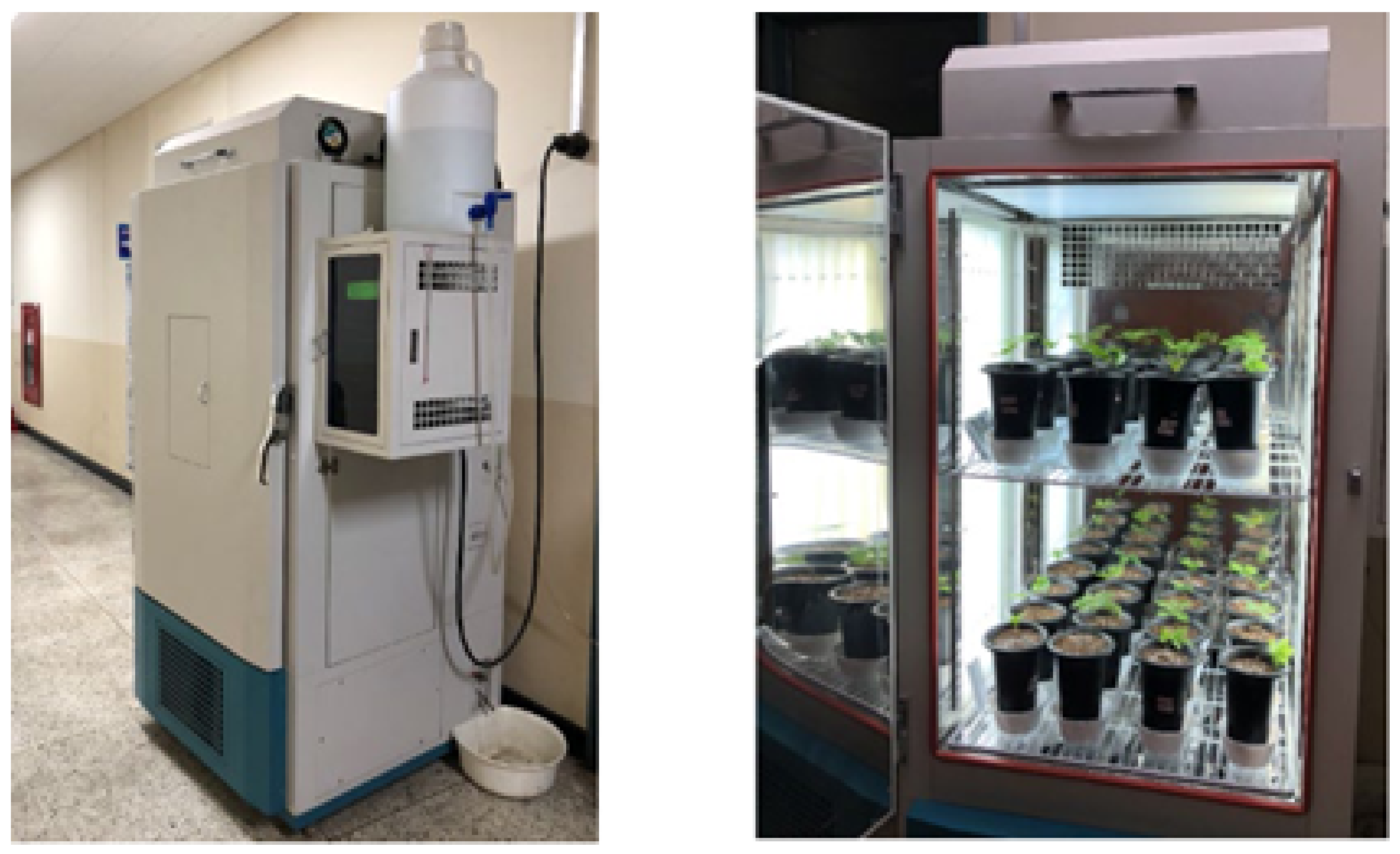
Korean ginseng (Panax ginseng Meyer) is a famous herbal plant that is sensitive to biotic stress. It is a shade-loving plant and useful for strengthening human immunity. It is highly sensitive to heat stress [11,12]. The roots of Korean ginseng have high pharmacological efficacy [13]. The size, appearance, and shape of the roots determine the quality and value of the roots. Generally, Ginseng plants are cultivated for several years, and the roots of the plants are harvested for sale between the fourth and sixth years. Ginseng roots are at risk of soil-borne diseases caused by nematodes, fungi, and bacteria in these long cultivation periods [14]. Among these fungi are the most common pathogens causing various diseases such as anthracnose, alternaria blight, root rot, gray mold, botrytis blight, etc. [15,16].
The fungus Cylindrocarpon destructans is one of the most harmful pathogens, causing root rot and rusty root disease. Root rot disease can significantly reduce ginseng production [17,18,19,20]. Cylindrocarpon destructans also gives rise to thick-walled resting spores known as chlamydospores that can survive for more than 10 years in the soil. This can lead to the development of root rot disease at any point of time while the spores remain in the soil [21].
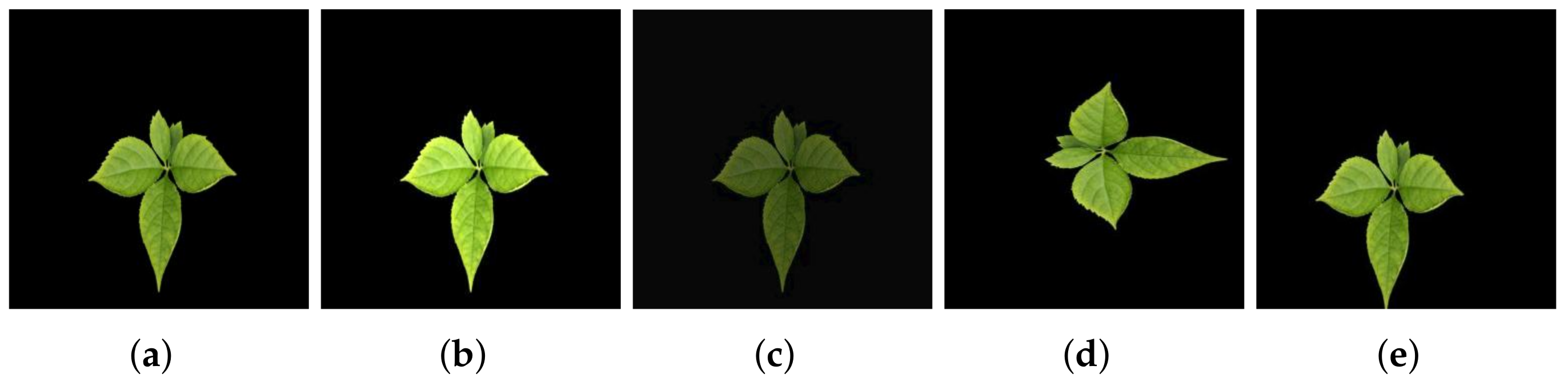
The root rot disease in grapevine plants cause symptoms in aboveground plant region [22,23,24]. These include stunted shoots, wilting leaves, low fruit production and dwarf leaves. Sometimes, the plants do not show any symptoms of disease (asymptomatic) in the aboveground plant region [23,25]. The roots cannot support the aboveground plant regions and they start to die. Hence, there will be less photosyntetic activities in the plants and the plant slowly starts to die. A study [26] on symptomatic and asymptomatic effects of this disease has been conducted in 15 plant species.
There are many existing methods [27,28] to identify the presence of Cylindrocarpon destructans, but these methods are destructive in nature. The root rot disease has been identified from the plant leaves using hyperspectral leaf images and machine learning techniques [25]. The root images are analyzed using feature extraction methods [29] and deep learning techniques [30] to find the root rot disease in Lentil. In order to obtain the root images, the plants are removed from the pots and the root images are captured.
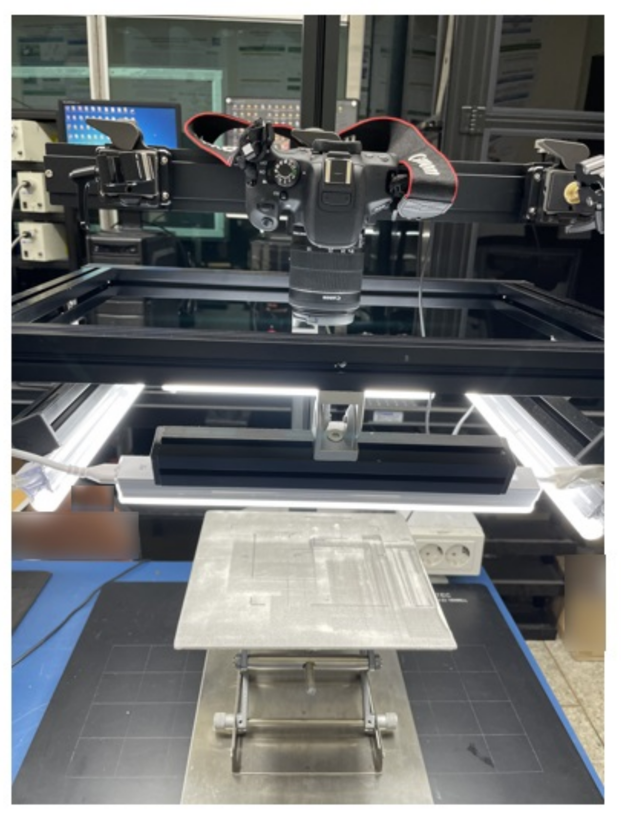
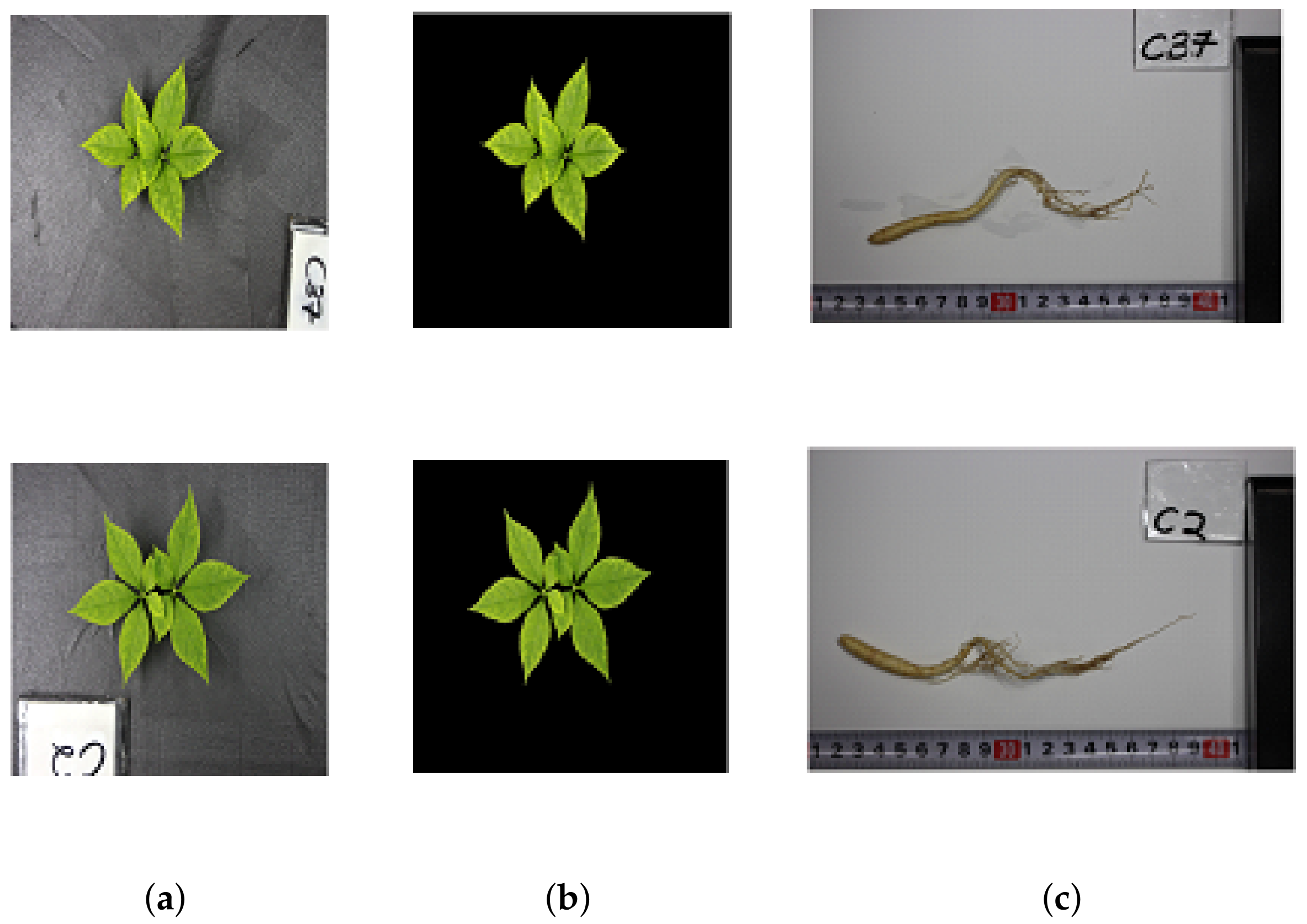
Hence, non-destructive identification of root rot disease is necessary to prevent a reduction in crop yield. In order to develop a low-cost, high-throughput, non-destructive, image-based analysis model, RGB images can be used. It is easy to collect numerous RGB images at a low cost and in a short time. Furthermore, various analyses are possible with these numerous data. The visible information from the collected RGB images helps in identifying the state and morphological changes in the plants through RGB-image-based plant phenotyping.
Nowadays, deep learning models are widely used to solve various complex real-time problems. Furthermore, their usage is increasing in solving agriculture-related problems. Among them are deep-learning-based plant phenotyping methods. The deep learning models can be applied to the collected data to perform various analyses.
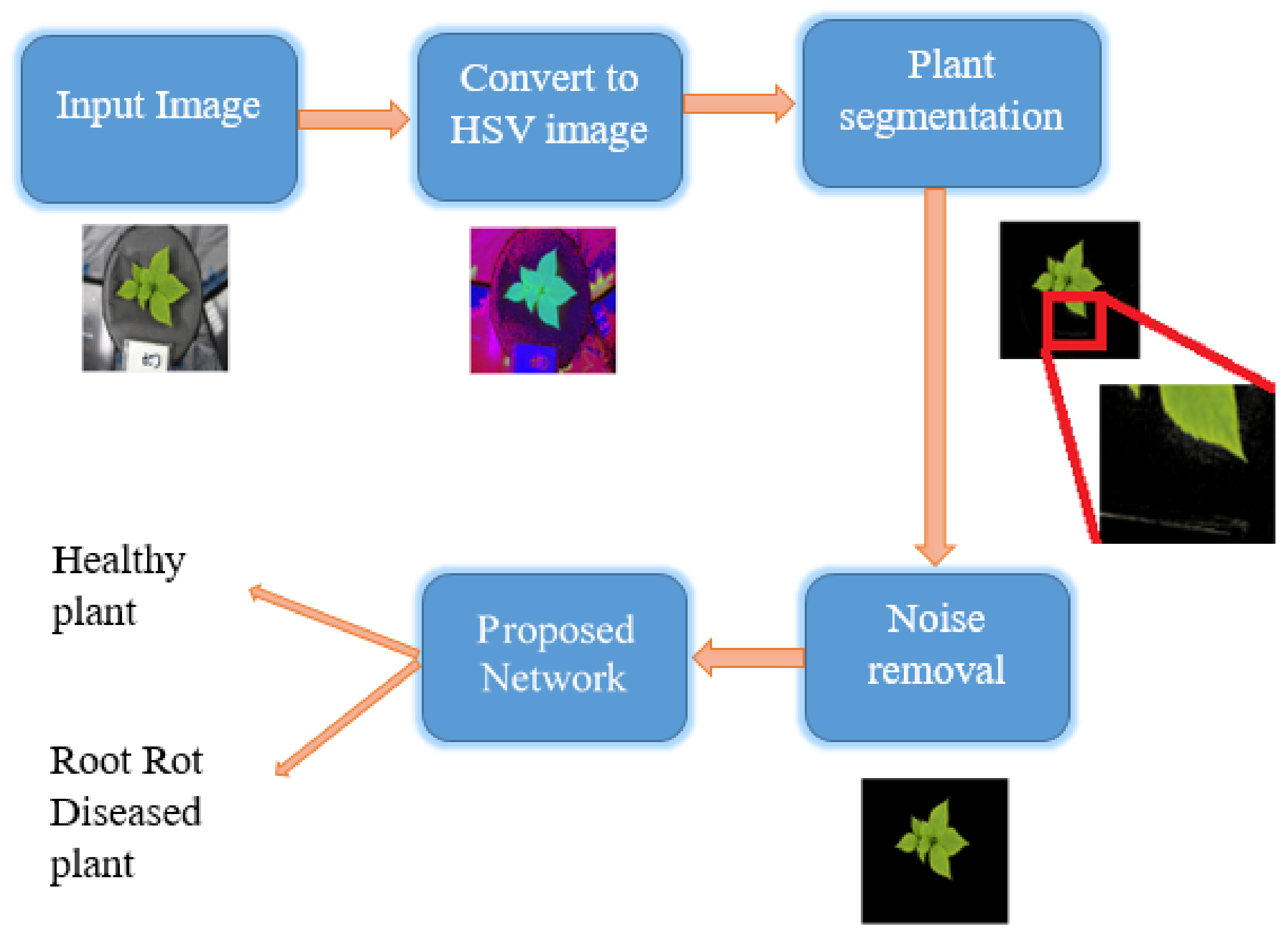
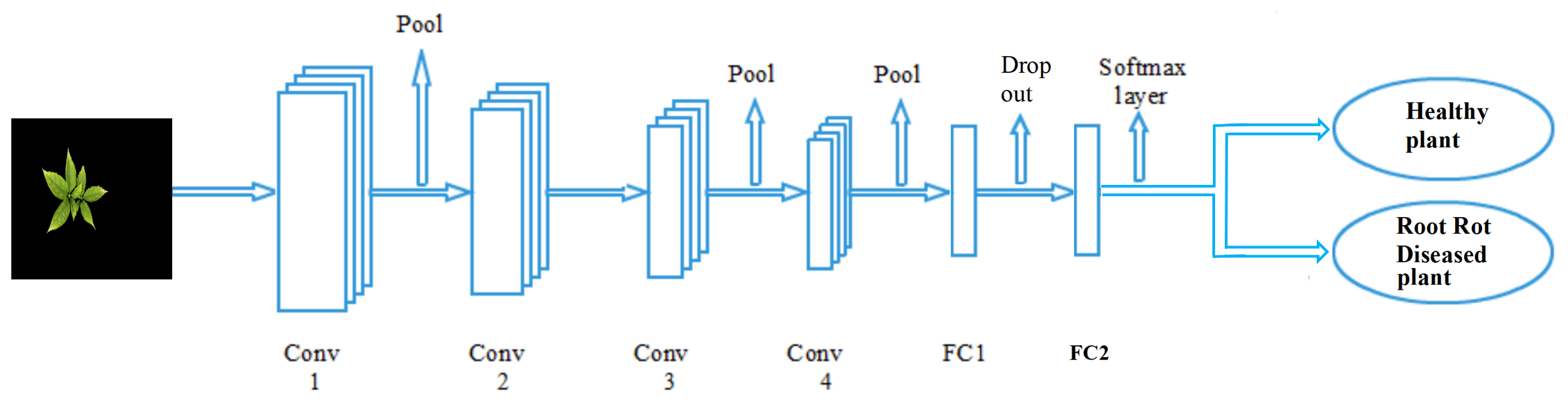
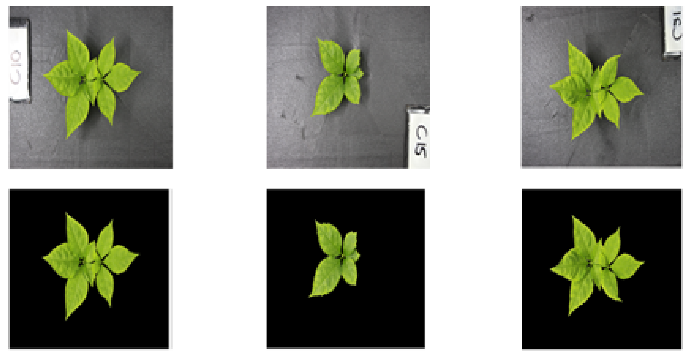
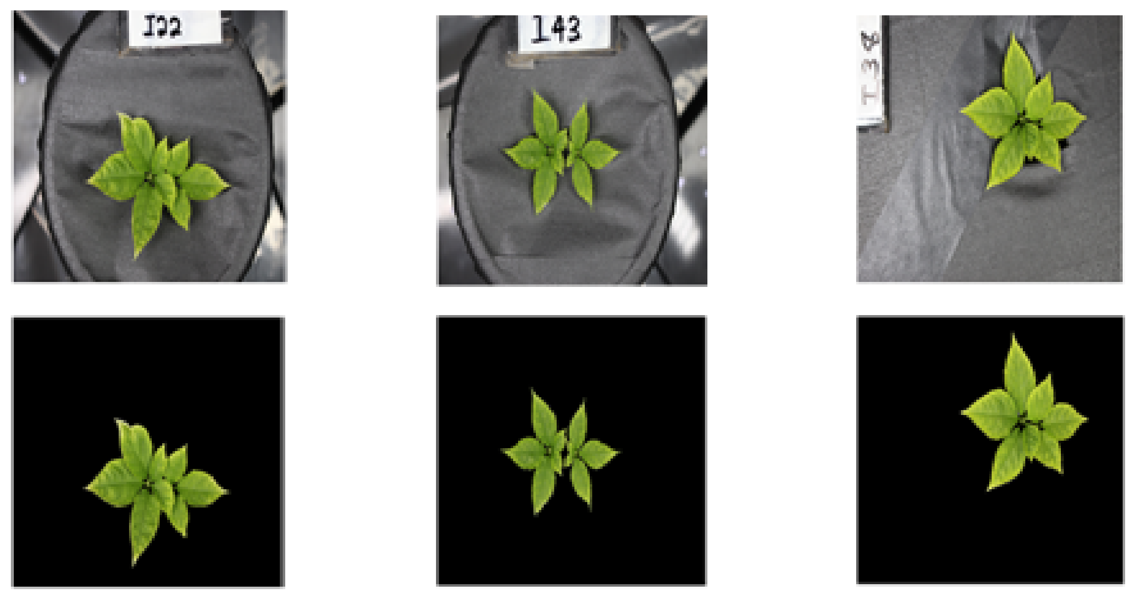
In the proposed method, various deep learning models are applied to identify biotically stressed (root rot) Korean ginseng plants based on RGB plant images. Furthermore, a new simple linear deep learning model is proposed. The proposed method involves three steps: (i) a region growing method for plant region segmentation, (ii) noise removal, and (iii) deep learning models for identifying biotically stressed (root rot) ginseng plants. In the first phase, the plant region is segmented from the raw RGB images using the seeded region growing method. Then, in the second step, the noise regions are removed from the segmented plant region. Finally, these noise-free segmented plant images are given as input to the proposed deep learning model to identify root-rot-diseased ginseng plants. The main advantages of the proposed method are that it (i) is non-destructive, (ii) is high throughput, (iii) does not require ground-truth images, (iv) is robust, and (v) is cost effective.
The structure of the remaining portion of this paper is as follows: Section 2 describes the materials and methods. Section 3 explains the results and provides a discussion, and finally, conclusions are given in Section 4.

2. Materials and Methods

2.1. Dataset Preparation

Dormant Panax ginseng roots were obtained from the Ginseng National Research Center in Daejeon, South Korea. After storage for 1 month at 4 degrees Celsius to break dormancy, the roots were planted in small pots. The soil used in our experiment was collected from the field and was contaminated with the soil-borne pathogen (Cylindrocarpon destructans) that causes root rot disease in ginseng plants. The collected soil was divided into two halves. One-half of the soil was sterilized using an autoclave [31]. The soil was sterilized at a temperature of 121 degrees Celsius for 20 min. The sterilization was repeated three times under similar conditions to ensure the healthiness of the soil. The plants were then grown in two different soil conditions: (i) pots containing the healthy soil and (ii) pots containing the soil mixed with soil-borne pathogens (Cylindrocarpon destructans). To grow the plants, the growing conditions were set to a temperature of 20 degrees Celsius with relative humidity of 60–70%, manual watering once a week, and continuous light intensity of 15,000 Lx. In our experiment, biotic stress was the only stress applied to the ginseng plants. Among the diseased plant images, the asymptotic diseased plant images [25] exist and did not show any symptoms in leaves but in roots. Figure 1 shows the plant growth conditions in the chamber.
RGB images of the ginseng plants were captured one day every week between the 10th week and 16th week using a Canon EOS 700D camera. The imaging device is shown in Figure 2. These images were stored in a computer separately for further analysis. The entire dataset of images was divided into training and testing images. There were 2112 healthy plant images and 1991 diseased plant images in the training dataset. The testing dataset contained 760 healthy plant images and 770 diseased plant images. Image augmentation [32,33] was adopted in our experiment. The variations such as Rotation in the range of ±180 degrees; Height and/or width shifting of ±0.1 of image dimensions; Contrast variation with the factor between 0.75 and 0.95; Illuminance variations with a factor of 0.5 and 1.5 are randomly applied. Figure 3 shows a few augmented images.
Of the training dataset, 10% were used for validation, and the remaining data in the training dataset were used for training the model. The images were carefully divided for training, validation, and testing such that plants in different stages were distributed evenly among the datasets in order to ensure that the proposed method is capable of identifying diseased plants at different stages. Once the images were collected during the 16th week, the plants were harvested to check the ginseng roots and root images were also captured in order to cross-verify the proposed model. The size of the plant and root images was 3456 × 5184.

2.2. Proposed Method

In a study conducted by Martínez-Ferri et al. [10], it was found that root rot disease has effects on the physiology of leaves. The authors in [25] studied the early identification of root rot disease in Grapevine. They identified the root rot disease by analyzing the hyperspectral images of the Grapevine leaves and matched the leaves symptoms with root symptoms. These studies motivated us to develop a high-throughput, non-destructive model that can be used to identify root rot disease from physiological changes in ginseng leaves. The proposed method consists of three steps. In the first step, the plant region is segmented based on the region growing algorithm. The purpose of plant segmentation is to improve the accuracy and robustness of the proposed method. In the second step, the noise regions are removed from the segmented plant regions. Finally, root rot disease is identified by the proposed deep learning model. The workflow for the proposed method is presented in Figure 4.

2.2.1. Plant Segmentation

In this step, the plant regions are segmented from the input plant images using the region growing algorithm. To segment the plant images, initially, the RGB plant images are resized into 227 × 227 × 3 and converted to HSV images. Then, the plant region is segmented based on Algorithm 1.
The selection criterion ( G i ) is given in the following equation:
G i = { 0.1 < H ( v i ) > 0.4 and S ( v i ) > 0.1 } ,
where H ( v i ) denotes the ith pixel value of the H plane and S ( v i ) denotes the ith pixel value of the S plane in the HSV plant image.
A pixel is considered a seed pixel (s) when it is the first occurring pixel that satisfies selection criterion G i in the HSV plant image. The similarity criterion plays a major role in the region growing process. This has to be chosen such that the plant region can be segmented from the plant image. In the proposed method, the similarity criterion ( G i , j ) was chosen as given in Equation (2):
G i , j = 1 , if G i and G j are true 0 , otherwise
where i and j are neighboring pixels of the plant image.
Equations (1) and (2) are used in the region growing algorithm (Algorithm 1) to segment the plant region.
Algorithm 1 Region growing method for plant segmentation
INPUT (I): HSV Plant image
OUTPUT (P): Segmented plant region
1:
B = Background region
2:
s = seed pixel
3:
G i , j = similarity criterion between the ith pixel and its non-visited neighboring jth pixel.
4:
G s , i = similarity criterion between the s and ith pixel.
5:
Initialize: P = { }, B = { } and G s , i =0.
6:
Select the seed pixel (s) as discussed in Section 2.2.1
7:
for each unassigned neighboring pixel of s do
8:
     G i , j = G i , j + G s , i
9:
    if  G i , j remains_unchanged then
10:
        Add that pixel to B
11:
        Search for a new seed pixel from the nearby unassigned pixels of the image.
12:
    else
13:
        Add that pixel to P
14:
        Update the current pixel as seed pixel.
15:
    end if
16:
end for
17:
Repeat until all pixels are assigned to either P or B

2.2.2. Noise Removal

The second step is noise removal from the segmented image. The segmented plant region contains certain background regions like the reflection of light, background pixels similar to the diseased portion, etc., as noise regions. These noise regions affect the root rot disease identification. Hence, it is very important to remove these noise regions. Utmost care should be taken in the noise removal stage because infected leaf regions may be removed along with the noise regions present in the segmented plant region. In the proposed method, the noise removal is done in the following way: (i) Initially, the connected components (similar pixels connected with each other) are identified in the segmented image. (ii) Then, the area of each component is calculated. (iii) Finally, the small objects are removed by thresholding. In the proposed method, based on experimentation, the threshold value was chosen to be 3500. After removing the noise region from the segmented region (P), it is mapped with the input HSV plane. There will be pixels in the HSV plane that do not map with P which are considered as background pixels. These background pixels are removed in HSV plane and the remaining plant region is used as the mask over the original RGB plant image to obtain the plant region.
Since the aim of the proposed method is to identify the root-rot-diseased plants (without ground truth images, so that it can be applied in various environments where the creation of ground truth images is tedious) and not plant segmentation, the segmentation accuracy was not calculated as this calculation requires ground truth images.

2.2.3. Root Rot Disease Identification

Once the plant regions are segmented from the plant images, they are given as the input to the proposed deep learning model to identify whether the plants are infected with root rot disease. Image augmentation techniques such as random rotation and random rescaling were used during the model training. The architecture of proposed model is shown in Figure 5, and the details are presented in Table 1. Furthermore, transfer learning models were used to identify the plants infected by root rot disease. In transfer learning, deep learning models are trained to learn the features in a domain and the models are optimized to learn more features in a specific domain. The various transfer learning models used in our experimentation were AlexNet, VGG19, SqueezeNet, DarkNet19, ResNet18, and ResNet101. In the proposed model, there are four convolutional layers. Three of these convolutional layers are followed by the maxpooling layer. All these layers are followed by two fully connected layers. The second fully connected layer is followed by a softmax layer and a classification layer. The numbers of neurons in the first and second fully connected layers are 1024 and 2, respectively.
The following is a brief discussion about the functions of the different layers in the deep learning models. The convolutional layer identifies the local feature maps from the input image. The size of the features can be calculated by the following equation:
F = [ ( W K + 2 P ) / S ] + 1
where F denotes the feature map size, W is the input image size, K is the filter size, P denotes the padding, and S denotes the stride.
The activation layer used in the proposed model is a ReLU layer. The ReLU function gives output the same as the input if the input is greater than 0. It is given by
R e L U ( x ) = m a x ( 0 , x )
where x is the input to the ReLU function.
Maxpooling is used to down-sample the obtained feature maps from the convolutional layer. The size of the output after maxpooling is given by the following equation:
O = f l o o r ( ( I y L ) / S )
where O is the output size of the maxpooling function, I y is the input shape, L is the pooling window size, and S is the stride.
The fully connected layers generate the final features by integrating the output of previous layers, and these final features are used for classification or regression. The softmax layer assigns the probabilities for each class in the problem. It is given by the following equation:
M ( x ) i = e x p ( x i ) j = 1 n e x p ( x j )
where M is the softmax, x is the input vector, and e x p ( x i ) and e x p ( x j ) are the exponential function for input and output vectors, respectively.
The classification layer calculates the loss and performs the classification tasks. The loss function used in the proposed model is cross-entropy. In our experiment, the loss function is given by the following equation:
L C = i = 1 2 l o g ( m i ) , f o r 2 c l a s s e s
where L C is the cross-entropy loss; t i is the truth value, having 0 or 1 as its value; and m i is the ith class softmax probability.
Table 1. Details of the proposed model Architecture.
LayerDetails
INPUT227 × 227 × 3
CONV116 3 × 3 filters with stride [1 1] and padding ‘same’
Maxpool13 × 3 max pooling with stride [2 2] and padding ‘same’
CONV232 3 × 3 filters with stride [1 1] and padding ‘same’
CONV332 3 × 3 filters with stride [1 1] and padding ‘same’
Maxpool23 × 3 max pooling with stride [2 2] and padding ‘same’
CONV48 3 × 3 filters with stride [1 1] and padding ‘same’
Maxpool33 × 3 max pooling with stride [2 2] and padding ‘same’
FC11 × 1 × 1024
Drop out0.5
FC21 × 1 × 2
Softmax1 × 1 × 2

3. Results and Discussion

The proposed method was implemented in Matlab (R2020b) on a system with a 64-bit Windows operating system, 16 GB memory, and a 2.9 GHz Intel i5 processor. Initially, the plant region was segmented from the plant images using Algorithm 1. Once the noise region was removed from the plant region, these images were given as input to the transfer learning models and the proposed model.

3.1. Performance Evaluation Measures

The measures used for evaluating the proposed model are as follows: (i) Precision (P) is the ratio of the number of correctly identified root-rot-diseased plants to the total number of identified root-rot-diseased plants. It is given in Equation (8). (ii) Recall (R) is the ratio of the number of correctly identified root-rot-diseased plants to the total number of root-rot-diseased plants. It is given in Equation (9). (iii) The F 1 score is the weighted average of P and R. It is given in Equation (10). (iv) Accuracy (Acc) is the proportion of correctly identified plants and is given by Equation (11).
P r e c i s i o n ( P ) = T P T P + F P
R e c a l l ( R ) = T P T P + F N
F 1 s c o r e = 2 × P × R P + R
A c c u r a c y = T P + F N T P + F N + F P + T N
Here, T P is True Positive, which denotes the number of root-rot-diseased plants correctly identified; F P is False Positive, which denotes the number of plants falsely identified as root rot diseased; F N is False Negative, which denotes the number of root-rot-diseased plants that were not identified as such; and T N denotes the number of healthy plants correctly identified.

3.2. Manual Design of Model: Effects of Layers and Hyperparameters

The proposed deep learning model was trained with the SGDM (Stochastic Gradient Descent with Momentum) solver. The values of the initial learning rate, number of epochs, batch size, and momentum were chosen as 0.001, 100, 64, and 0.9, respectively. These parameter values were chosen such that the model has high performance. The manual selection involved in designing the architecture is explained as follows.

3.2.1. Layers

In designing the proposed model, the appropriate layers were selected in such a way that the model exhibited better classification accuracy. The proposed model was also tested with fewer layers and more layers. The model did not learn the necessary root rot disease features when designed with fewer layers, resulting in lower accuracy, whereas the model learned more features but showed overfitting when it was designed with more layers. In our design, combinations such as (Conv2, Pool2), (Conv3, Pool2), (Conv4, Pool2), (Conv4, Pool3), (Conv5, Pool2), (Conv5, Pool3), (Conv6, Pool2) and (Conv6, Pool3) were evaluated. The high accuracy and low error was achieved when the number of convolution layers was increased from two to four and the number of pooling layers used was three. However, when the number of layers was increased, the accuracy was reduced. Hence, a further increase in the number of layers did not have a significant effect on the accuracy. Thenmozhi and Srinivasulu Reddy [34] studied the effects of the number of layers in the performance of their model. They investigated the layer depth of the CNN model and analyzed the effect of the number of layers in their model for pest classification by varying the number of convolution layers from three to seven. They observed that the accuracy decreased with an increase in the number of layers, and lower error was observed for six convolution and five pooling layers, avoiding the occurrence of degradation. It can be observed from Table 2 that the proposed model performed better for four convolution and three pooling layers and effectively reduced overfitting.

3.2.2. Number of Epochs

The proposed model was trained for up to 100 epochs. The initial learning rate and mini-batch size were set to 0.001 and 64, respectively. The accuracy and loss curves during model training is shown in Figure 6. It can be observed from both the curves that the loss values are stable, and after the 75th epoch the accuracy results are closer to 100% with less fluctuation for training and closer to 90% for validation and obtaining 90.73% at 100th epoch.

3.2.3. Initial Learning Rate

The initial learning rate is one of the key factors that determines model performance. The learning process speed is high when the model is trained with a higher learning rate, but there will be an increase in the loss function. The loss function can be decreased with a lower learning rate. Hence, it is essential to set the appropriate learning rate when training a model. Xia et al. [35] performed a study on pest classification and varied the initial learning rate between 0.0006 and 0.0014; the best performance was obtained at an initial learning rate of 0.0001. In our experiment, the proposed model was evaluated with various initial learning rate values, such as 0.000001, 0.00001, 0.0001, 0.001, and 0.01. The number of epochs and size of mini-batches were set to 100 and 64, respectively, during the evaluation of the model. The performance evaluation is shown in Table 3. It can be observed from Table 3 that the proposed model performed better when the initial learning rate was set to 0.001.

3.2.4. Mini-Batch Size

The mini-batch size is an important parameter when training a deep learning model. The model takes a long time and huge memory to run if the batch size is larger. Hence, it is essential to select the appropriate mini-batch size for better performance of deep learning models [36]. In our experiment, the proposed model was evaluated with various sizes of mini-batches, such as 1, 16, 32, 64, 128, and 256. The performance of the proposed model is high with the mini-batch size of 64. This is shown in Table 4. The proposed model was evaluated for 100 epochs with a learning rate of 0.001. Based on the experiment, a mini-batch size of 64 was chosen to train proposed model such that the convergence precision of proposed model is increased. It can be observed from Table 4 that a further increase in mini-batch size did not improve the model performance. Hence, the proposed model was trained with a mini-batch size of 64.

3.3. Machine Learning Based Optimization in Designing the Model

The manual hyperparameter designing in a model has a few limitations such as the dependency of knowledge and experience of the users, time consuming to find the optimal hyperparameters, and difficulty in handling huge data when the number of parameters and their range of values increase. The users require the capacity to identify the relations between the hyperparameters and the results obtained through visualization tools [37]. In order to overcome these limitations, machine learning based hyperparameter optimization has been used in recent researches. One among them is bayesian optimization [38]. This was used in our experiment and the initial learning rate and batch size were set to 0.0006 and 64, respectively. The number of epoch was set to 82.
The performance evaluation of the model with manual selection and machine learning based optimization is given in Table 5. It is observed from Table 5 the performance of the model is increased with machine learning based optimization. Hence, this result is used to compare with the other models.

3.4. Overall Performance of Proposed Model for Root Rot Disease Identification in Ginseng Plants

The plant regions were initially segmented from the healthy and diseased plant images as shown in Figure 7 and Figure 8, respectively. The time taken for the proposed segmentation method was less than 5 s per image. After segmenting the plant region, the root rot disease identification was performed by transfer learning models and proposed model. Sample plant images that were correctly identified by proposed model are shown in Figure 9 and Figure 10. These figures show that the leaves and roots of the healthy and diseased plants have a major difference in their appearance. It can be observed from these figures that the diseased plants have shorter primary roots, whereas the length of the primary roots in the healthy plants is greater than that in the diseased plants. Furthermore, it can be observed that there are many secondary and tertiary roots in healthy plants, but there are no such roots in the diseased plants. The healthy and root-rot-diseased plants were identified in a promising manner by proposed model. This shows the performance of the proposed model in identifying root rot disease in ginseng plants.
The Figure 11 shows sample images on which proposed model failed. There exist a few asymptotic plants in the dataset. They do not show any symptoms in leaf but infected by the pathogens. The proposed model fails to identify these plants as shown in Figure 12. The times taken for training the transfer learning models and the proposed model are given in Table 6. In order to analyze the improvement in model performance due to plant segmentation, the deep learning models were also tested with raw plant images as input. The performance of the deep learning models is given in Table 7 and Table 8.
Table 7 and Table 8 show that the deep learning models performed well when the segmented plant images were given as input. It is observed from Table 6 that the proposed model required less training time when compared with a few transfer learning models except Resnet-18 and Squeezenet. Furthermore, the inference time of proposed model is lower than the other models as shown in Table 9. It is observed from Table 10 that the number of parameters of proposed model are less when compared with other models. These show that the proposed model can be practically applicable in a high-throughput system.
The proposed model achieved a high precision value of 0.95 and a recall value of 0.82. Additionally, it achieved a high F 1 score of 0.88 and accuracy of 0.89, which are higher than those of the other transfer learning models. These imply that the proposed proposed can accurately predict 89% of diseased plants in the created dataset. Furthermore, the training time and inference time of proposed model are comparatively lower, increasing the practicality of this model. Overall, the proposed model has several advantages in real-time deployment.

4. Conclusions

In this paper, a new deep learning model was proposed to identify root rot disease in ginseng plants. Initially, the plant regions are segmented using the region growing method, and then the noise in the segmented plant regions is removed. Finally, the root-rot-diseased plants are identified by the proposed model. The performance of proposed model was compared with that of transfer learning models. The proposed model achieved an F 1 score of 0.88 and accuracy of 0.89 in less inference time when compared with the transfer learning models. Overall, the proposed model has several advantages, such as high throughput, cross-platform applicability, and robustness. However, a further improvement in performance is required, as well as the early detection of disease. This can be achieved by using various imaging sensors such as hyperspectral, fluorescence, etc., and corresponding image analysis methods. Additionally, this experiment can be improved by applying various plant stresses along with root rot disease.

Author Contributions

Conceptualization, P.K.J. and B.-K.C.; data curation, E.P., M.A.F. and Y.-S.K.; data analysis, P.K.J., H.K., I.B., M.S.K. and B.-K.C.; model development, P.K.J., H.K., D.S. and B.-K.C.; writing—original draft, P.K.J. and B.-K.C.; writing—review and editing, B.-K.C.; supervision, B.-K.C. All authors have read and agreed to the published version of the manuscript.

Funding

This research was supported by a grant from the Korean Society of Ginseng Funded by Korean Ginseng Corporation.

Institutional Review Board Statement

Not applicable.

Informed Consent Statement

Not applicable.

Data Availability Statement

Not applicable.

Conflicts of Interest

The authors declare no conflict of interest.

References

  1. Minervini, M.; Scharr, H.; Tsaftaris, S. Image analysis: The new bottleneck in plant phenotyping [applications corner]. IEEE Signal Process. Mag. 2015, 32, 126–131. [Google Scholar] [CrossRef] [Green Version]
  2. Furbank, R.T.; Tester, M. Phenomics—Technologies to relieve the phenotyping bottleneck. Trends Plant Sci. 2011, 16, 635–644. [Google Scholar] [CrossRef]
  3. Wu, B.; Nevatia, R. Detection and segmentation of multiple, partially occluded objects by grouping, merging, assigning part detection responses. Int. J. Comput. Vis. 2009, 82, 185–204. [Google Scholar] [CrossRef] [Green Version]
  4. Kumar, P.; Domnic, S. Computer Vision for Green Plant Segmentation and Leaf Count. In Modern Techniques for Agricultural Disease Management and Crop Yield Prediction; IGI Global: Hershey, PA, USA, 2020; pp. 89–110. [Google Scholar]
  5. Kumar, J.P.; Domnic, S. Rosette plant segmentation with leaf count using orthogonal transform and deep convolutional neural network. Mach. Vis. Appl. 2020, 31, 1–14. [Google Scholar]
  6. Dellen, B.; Scharr, H.; Torras, C. Growth signatures of rosette plants from time-lapse video. IEEE/ACM Trans. Comput. Biol. Bioinform. 2015, 12, 1470–1478. [Google Scholar] [CrossRef] [PubMed] [Green Version]
  7. Grand-Brochier, M.; Vacavant, A.; Cerutti, G.; Kurtz, C.; Weber, J.; Tougne, L. Tree leaves extraction in natural images: Comparative study of preprocessing tools and segmentation methods. IEEE Trans. Image Process. 2015, 24, 1549–1560. [Google Scholar] [CrossRef] [Green Version]
  8. Legendre, R.; Basinger, N.T.; van Iersel, M.W. Low-Cost Chlorophyll Fluorescence Imaging for Stress Detection. Sensors 2021, 21, 2055. [Google Scholar] [CrossRef] [PubMed]
  9. Khanna, R.; Schmid, L.; Walter, A.; Nieto, J.; Siegwart, R.; Liebisch, F. A spatio temporal spectral framework for plant stress phenotyping. Plant Methods 2019, 15, 1–18. [Google Scholar] [CrossRef] [Green Version]
  10. Martínez-Ferri, E.; Zumaquero, A.; Ariza, M.; Barceló, A.; Pliego, C. Nondestructive detection of white root rot disease in avocado rootstocks by leaf chlorophyll fluorescence. Plant Dis. 2016, 100, 49–58. [Google Scholar] [CrossRef] [Green Version]
  11. Jayakodi, M.; Lee, S.C.; Yang, T.J. Comparative transcriptome analysis of heat stress responsiveness between two contrasting ginseng cultivars. J. Ginseng Res. 2019, 43, 572–579. [Google Scholar] [CrossRef]
  12. Lee, J.S.; Lee, J.H.; Ahn, I.O. Characteristics of resistant lines to high-temperature injury in ginseng (Panax ginseng CA Meyer). J. Ginseng Res. 2010, 34, 274–281. [Google Scholar] [CrossRef] [Green Version]
  13. Lee, S.M.; Bae, B.S.; Park, H.W.; Ahn, N.G.; Cho, B.G.; Cho, Y.L.; Kwak, Y.S. Characterization of Korean Red Ginseng (Panax ginseng Meyer): History, preparation method, and chemical composition. J. Ginseng Res. 2015, 39, 384–391. [Google Scholar] [CrossRef] [Green Version]
  14. Yu, Y.; Ohh, S. Research on ginseng diseases in Korea. Korean J. Ginseng Sci. 1993, 17, 61–68. [Google Scholar]
  15. Farh, M.E.A.; Kim, Y.J.; Kim, Y.J.; Yang, D.C. Cylindrocarpon destructans/Ilyonectria radicicola-species complex: Causative agent of ginseng root-rot disease and rusty symptoms. J. Ginseng Res. 2018, 42, 9–15. [Google Scholar] [CrossRef]
  16. Park, Y.H.; Kim, Y.C.; Park, S.U.; Lim, H.S.; Kim, J.B.; Cho, B.K.; Bae, H. Age-dependent distribution of fungal endophytes in Panax ginseng roots cultivated in Korea. J. Ginseng Res. 2012, 36, 327. [Google Scholar] [CrossRef] [Green Version]
  17. Reeleder, R.; Brammall, R. Pathogenicity of Pythium species, Cylindrocarpon destructans, and Rhizoctonia solani to ginseng seedlings in Ontario. Can. J. Plant Pathol. 1994, 16, 311–316. [Google Scholar] [CrossRef]
  18. Kang, Y.; Kim, M.R.; Kim, K.H.; Lee, J.; Lee, S.H. Chlamydospore induction from conidia of Cylindrocarpon destructans isolated from ginseng in Korea. Mycobiology 2016, 44, 63–65. [Google Scholar] [CrossRef] [Green Version]
  19. Chung, H.S. Studies on Cylindrocarpon destructans (Zins.) Scholten causing root rot of ginseng. Rep. Tottori Mycol. Inst. 1975, 12, 127–138. [Google Scholar]
  20. Cho, D.H.; Park, K.J.; Yu, Y.H.; Ohh, S.; Lee, H. Root-rot development of 2-year old ginseng (Panax ginseng CA Meyer) caused by Cylindrocarpon destructans (Zinssm.) Scholten in the continuous cultivation field. Korean J. Ginseng Sci. 1995, 19, 175–180. [Google Scholar]
  21. Cho, D.H.; Yu, Y.H.; Kim, Y.H. Morphological characteristics of chlamydospores of Cylindrocarpon destructans causing root-rot of Panax ginseng. J. Ginseng Res. 2003, 27, 195–201. [Google Scholar]
  22. Ricciolini, M.; Rizzo, D. Avversità della Vite e Strategie di Difesa Integrata in Toscana; Press Service srl: Sesto Fiorentino, Italy, 2007. [Google Scholar]
  23. Baumgartner, K.; Rizzo, D.M. Spread of Armillaria root disease in a California vineyard. Am. J. Enol. Vitic. 2002, 53, 197–203. [Google Scholar]
  24. Daniele; Prodorutti, F.; de Luca, A.; Pellegrini, I.; Pertot. I Marciumi Radicali Della Vite; Safe Crop: San Michele all’Adige, Italy, 2007. [Google Scholar]
  25. Calamita, F.; Imran, H.A.; Vescovo, L.; Mekhalfi, M.L.; La Porta, N. Early Identification of Root Rot Disease by Using Hyperspectral Reflectance: The Case of Pathosystem Grapevine/Armillaria. Remote Sens. 2021, 13, 2436. [Google Scholar] [CrossRef]
  26. Kolander, T.; Bienapfl, J.; Kurle, J.; Malvick, D. Symptomatic and asymptomatic host range of Fusarium virguliforme, the causal agent of soybean sudden death syndrome. Plant Dis. 2012, 96, 1148–1153. [Google Scholar] [CrossRef] [PubMed] [Green Version]
  27. Jang, C.S.; Lim, J.H.; Seo, M.W.; Song, J.Y.; Kim, H.G. Direct Detection of Cylmdrocarpon destructans, Root Rot Pathogen of Ginseng by Nested PCR from Soil Samples. Mycobiology 2010, 38, 33–38. [Google Scholar] [CrossRef] [Green Version]
  28. Seifert, K.; McMullen, C.; Yee, D.; Reeleder, R.; Dobinson, K. Molecular differentiation and detection of ginseng-adapted isolates of the root rot fungus Cylindrocarpon destructans. Phytopathology 2003, 93, 1533–1542. [Google Scholar] [CrossRef] [PubMed] [Green Version]
  29. Marzougui, A.; Ma, Y.; Zhang, C.; McGee, R.J.; Coyne, C.J.; Main, D.; Sankaran, S. Advanced imaging for quantitative evaluation of Aphanomyces root rot resistance in lentil. Front. Plant Sci. 2019, 10, 383. [Google Scholar] [CrossRef] [Green Version]
  30. Marzougui, A.; Ma, Y.; McGee, R.J.; Khot, L.R.; Sankaran, S. Generalized Linear Model with Elastic Net Regularization and Convolutional Neural Network for Evaluating Aphanomyces Root Rot Severity in Lentil. Plant Phenomics 2020, 2020, 2393062. [Google Scholar] [CrossRef]
  31. Werner, H.; Kindt, R.; Borneff, J. Testing the sterilisation effect of autoclaves by means of biological indicators (author’s transl). Zentralblatt Fur Bakteriol. Parasitenkd. Infekt. Hyg. Erste Abt. Orig. Reihe B Hyg. Prav. Med. 1975, 160, 458–472. [Google Scholar]
  32. Kutlugün, M.A.; Sirin, Y.; Karakaya, M. The effects of augmented training dataset on performance of convolutional neural networks in face recognition system. In Proceedings of the 2019 Federated Conference on Computer Science and Information Systems (FedCSIS), Leipzig, Germany, 1–4 September 2019; pp. 929–932. [Google Scholar]
  33. Naranjo-Torres, J.; Mora, M.; Hernández-García, R.; Barrientos, R.J.; Fredes, C.; Valenzuela, A. A review of convolutional neural network applied to fruit image processing. Appl. Sci. 2020, 10, 3443. [Google Scholar] [CrossRef]
  34. Thenmozhi, K.; Reddy, U.S. Crop pest classification based on deep convolutional neural network and transfer learning. Comput. Electron. Agric. 2019, 164, 104906. [Google Scholar] [CrossRef]
  35. Xia, D.; Chen, P.; Wang, B.; Zhang, J.; Xie, C. Insect detection and classification based on an improved convolutional neural network. Sensors 2018, 18, 4169. [Google Scholar] [CrossRef] [PubMed] [Green Version]
  36. Lee, M.; Xing, S. A study of tangerine pest recognition using advanced deep learning methods. Preprints 2018, 2018110161. [Google Scholar] [CrossRef]
  37. Jain, A. Complete Guide to Parameter Tuning in Gradient Boosting (Gbm) in Python. Analyticsvidhya.com. 2016. Available online: https://www.analyticsvidhya.com/blog/2016/02/complete-guide-parametertuning-gradient-boosting-gbm-python (accessed on 14 January 2022).
  38. Wu, J.; Chen, X.Y.; Zhang, H.; Xiong, L.D.; Lei, H.; Deng, S.H. Hyperparameter optimization for machine learning models based on Bayesian optimization. J. Electron. Sci. Technol. 2019, 17, 26–40. [Google Scholar]
Figure 1. Plant growth chamber.
Applsci 12 02489 g001
Figure 2. Imaging device.
Applsci 12 02489 g002
Figure 3. Data augmentation. (a) Original plant image; (b) Image with Contrast variation; (c) Image with Illuminance variation; (d) Rotated image; (e) Height and/or width shifted image.
Applsci 12 02489 g003
Figure 4. Workflow of the proposed method.
Applsci 12 02489 g004
Figure 5. The proposed model Architecture.
Applsci 12 02489 g005
Figure 6. Accuracy and Loss curves during model training.
Applsci 12 02489 g006
Figure 7. Plant segmentation from healthy plant images. The top row presents raw plant images; the bottom row presents segmented plant images.
Applsci 12 02489 g007
Figure 8. Plant segmentation from diseased plant images. The top row presents raw plant images; the bottom row presents segmented plant images.
Applsci 12 02489 g008
Figure 9. Correct identification of healthy plants by proposed model. (a) Raw plant; (b) Segmented plant region; (c) Plant root.
Applsci 12 02489 g009
Figure 10. Correct identification of diseased plants by proposed model. (a) Raw plant; (b) Segmented plant region; (c) Plant root.
Applsci 12 02489 g010
Figure 11. Incorrect identification of diseased plants by proposed model. (a) Raw plant; (b) Segmented plant region; (c) Plant root.
Applsci 12 02489 g011
Figure 12. Incorrect identification of diseased plant images. The top row presents raw images; the bottom row presents segmented images.
Applsci 12 02489 g012
Table 2. Performance evaluation of proposed model for different numbers of layers.
Layer CombinationsAccuracy (%)
Conv2Pool278.76
Conv3Pool283.59
Conv4Pool288.17
Conv4Pool390.73
Conv5Pool286.86
Conv5Pool385.49
Conv6Pool284.64
Conv6Pool383.26
Table 3. Performance evaluation of proposed model for various initial learning rates.
Learning RateAccuracy (%)
0.00000185.16
0.0000187.06
0.000188.04
0.00190.73
0.0178.76
Table 4. Performance evaluation of proposed model for various mini-batch sizes.
Mini-Batch SizeAccuracy (%)
185.16
1685.95
3288.04
6490.73
12887.12
25686.47
Table 5. Performance evaluation of proposed model: Manual selection Vs Machine learning based optimization.
Method for Model DesignAccuracy (%)-Validation DataAccuracy (%)-Test Data
Manual selection90.7387.78
Machine learning based optimization93.8689.02
Table 6. Training times of various deep learning models.
Deep Learning ModelTraining Time
Alexnet25 min 46 s
VGG1954 min 32 s
Squeezenet7 min 16 s
Darknet1950 min 57 s
Resnet1812 min 51 s
Resnet10194 min 35 s
Proposed model18 min 11 s
Table 7. Performance comparison of various deep learning models with raw plant images (from testing dataset) as input.
Deep Learning ModelPrecisionRecall F 1 ScoreAccuracy
Alexnet0.600.870.710.64
VGG190.640.910.750.69
Squeezenet0.640.930.760.71
Darknet190.640.930.760.71
Resnet180.660.950.780.73
Resnet1010.630.890.740.68
Proposed model0.640.920.760.70
Table 8. Performance comparison of various deep learning models with segmented plant regions (from testing dataset) as input images.
Deep Learning ModelPrecisionRecall F 1 ScoreAccuracy
Alexnet0.890.820.850.86
VGG190.870.840.850.85
Squeezenet0.890.770.830.84
Darknet190.890.770.830.84
Resnet180.880.840.860.86
Resnet1010.880.780.830.84
Proposed model0.950.820.880.89
Table 9. Inference times (for testing dataset) of various deep learning models.
Deep Learning ModelInference Time
Alexnet13.15 s
VGG1921.63 s
Squeezenet14.41 s
Darknet1919.45 s
Resnet1817.39 s
Resnet10135.93 s
Proposed model8.97 s
Table 10. Parameters of various deep learning models.
Deep Learning ModelParameters
Alexnet61 M
VGG19138 M
Squeezenet12 M
Darknet1922 M
Resnet1811 M
Resnet10144 M
Proposed model6 M
Publisher’s Note: MDPI stays neutral with regard to jurisdictional claims in published maps and institutional affiliations.

