Fast and Efficient Union of Sparse Orthonormal Transforms via DCT and Bayesian Optimization ^†

Abstract

Sparse orthonormal transform is based on orthogonal sparse coding, which is relatively fast and suitable in image compression such as analytic transforms with better performance. However, because of the constraints on its dictionary, it has performance limitations. This paper proposes an extension of a sparse orthonormal transform based on unions of orthonormal dictionaries for image compression. Unlike unions of orthonormal bases (UONB), which implement an overcomplete dictionary with several orthonormal dictionaries, the proposed method allocates patches to an orthonormal dictionary based on their directions. The dictionaries are constructed into a discrete cosine transform and an orthonormal matrix. To determine a trade-off parameter between the reconstruction error and sparsity, which hinders efficient implementation, the proposed method adapts Bayesian optimization. The framework exhibits an improved performance with fast implementation to determine the optimal parameter. It is verified that the proposed method performs similar to an overcomplete dictionary with a faster speed via experiments.

1. Introduction

Sparse coding is a machine-learning technique that represents data as a linear combination of a few atoms. As an important tool, it has been widely used in many signal and image processing applications in the past decades [1,2,3]. However, unlike other applications, sparse coding has not been practically used in image compression, although many studies have designed transforms for compression or transform coding schemes to be used for compression standards [4]. One of the main reasons for its limited use is that existing analytic transforms such as discrete cosine transform (DCT) or Fourier transform exhibit adequate performance with fast implementation, whereas sparse coding techniques require high computational costs for optimizations, although they perform better than analytic transforms. However, many attempts have been made to formulated transforms via sparse coding [5,6,7,8]. The general formulation of the sparse coding is as follows.

$$\underset{D,A}{\min }\left\{{∥X-DA∥}_F^2+\lambda {∥A∥}_0\right\},$$

(1)

Here, $D\in {\mathbb{R}}^{n\times m}$ is an overcomplete dictionary ($m>n$) and $A\in {\mathbb{R}}^{m\times N}$ is the sparse coefficient.

In [4,9], sparse orthonormal transforms (SOTs) were designed using an orthogonal sparse coding methodology. Orthogonal sparse coding was formulated with an orthonormal constraint on the dictionary structure. In Equation (1), the dictionary D does not have any constraints, but it is usually non-square and non-orthogonal. The orthonormal constraint helps reduce the computational burden of sparse coding in the optimization procedure. Owing to the orthonormal constraint, the form and properties of the dictionary are similar to those of analytic transforms because it represents the input signal with a minimal basis. Sezer et al. [4,9] formulated a transform with an orthonormal matrix and an L₀ norm constraint on the transform coefficients. The transform is easily invertible by its transpose matrix and satisfies Parseval’s theorem. They also theoretically proved that the transform is superior to the existing analytic transform, especially Karhunen–Loeve Transform (KLT). It is important because KLT is a well-known optimal transform in the Gaussian process. They show that the SOT is identical to KLT in the Gaussian process and outperforms it in the non-Gaussian process. This SOT heuristically gives better performance than other image orthonormal transforms. However, the performance of the orthonormal dictionary was adequate but not comparable to that of an overcomplete dictionary. The large and wide dictionary could represent sparser and more redundant data. In addition, the orthogonal sparse coding is much faster than the overcomplete coding, but the computation is still slow because of the high number of iterations. In this paper, we extend the SOT to be applied to an overcomplete dictionarywhile reducing the computational time. We also propose a method to find a parameter $\lambda$ in Equation (1) for efficient implementation. Since the performance of sparse coding is sensitive to $\lambda$, the use of an optimal $\lambda$ is important.

Our method uses multiple dictionaries to outperform the SOT. Ref. [10] first proposed a sparse coding methodology with multiple dictionaries. The method named union of orthonormal bases (UONB) implements an overcomplete dictionary with several orthogonal dictionaries, and it can find an overcomplete dictionary faster. In this study, we used multiple dictionaries in a different way from [10], because the problem in this study is different from that in [10]. We based our transform on an orthogonal dictionary, such as the SOT. Instead, we classified the image patches and allocated each group to one orthogonal dictionary. Then, we converted the problem into a multiple orthogonal sparse coding problem.

To classify input patches and create an efficient framework, we exploited a discrete cosine transform. Before allocating dictionaries, our method requires the construction of a subdataset. We assumed that a dataset with similar directional patches helps design suitable dictionaries. In our method, we exploited the edge detection method in the DCT domain [11]. Then, the DCT matrix is also used to prevent increasing the computational times of the usage of multiple dictionaries.

In sparse coding, using an appropriate value of $\lambda$ is also important. This value affects the performance. However, because the optimal value is not convex and varies for target sparsity, finding the optimal value is difficult. Thus, efficient implementation requires finding $\lambda$ quickly. In our previous work [12], we used an exhaustive method (or greedy search) to find it for each sparsity level. In [4], the authors proposed a method to gradually reduce the step size for iterations. In this study, we resolved the problem via Bayesian optimization [13,14]. As a type of global optimization method, Bayesian optimization can find a near-optimal value in a non-convex function.

Our contributions can be summarized as follows:

• The SOT provides powerful transform, which outperforms KLT, but it is limited because of the computation time and dictionary size.
• We propose an extension of the SOT to address the limitation of orthonormal dictionary learning, which is based on the union of orthonormal bases. However, in contrast to [10], we formulated an orthogonal sparse coding in several orthogonal sparse coding problems with subdatasets.
• We classified input data and allocate each orthogonal dictionary and its coefficients to each classified input data to help to make the input data sparse representation.
• To prevent time and iteration increase by the number of dictionaries, we used a double-sparsity structure proposed in [15] with a DCT matrix as a fixed base dictionary.
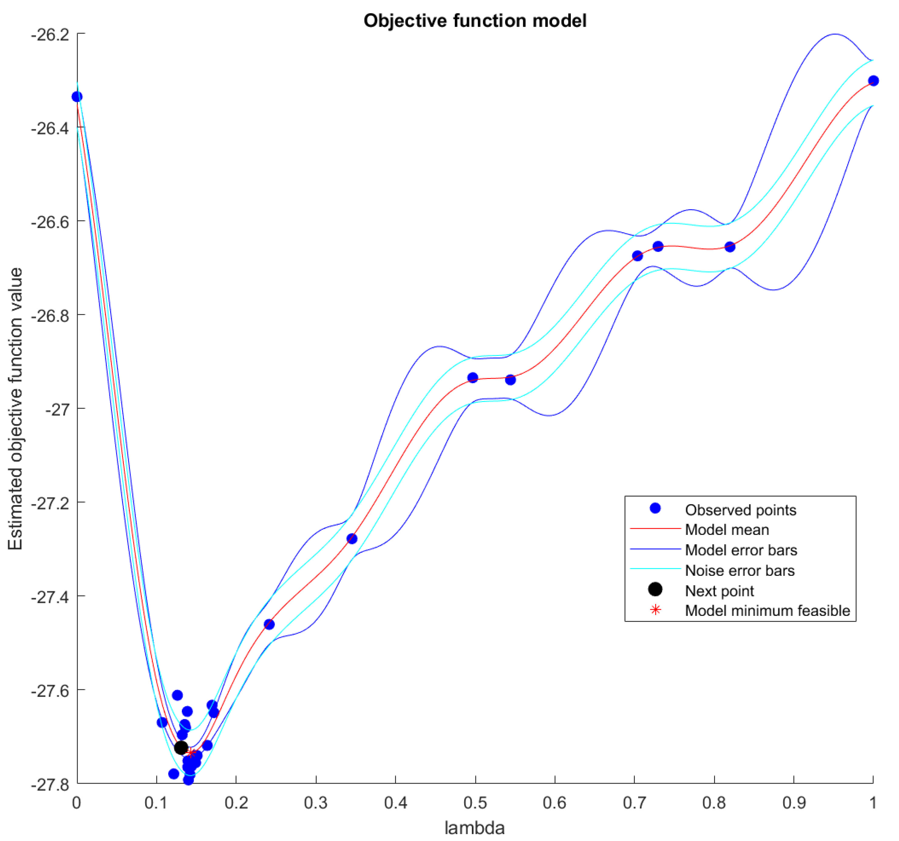
• To find the optimal value of $\lambda$, which is non-convex and continuous, we adapted Bayesian optimization in our proposed method and set the optimal parameter with fewer iterations.

Thus, we propose a framework to design transforms that outperform the SOT in a short time.

2. Related Works

2.1. Sparse Orthonormal Transform

For sparse coding based on an overcomplete dictionary, finding an appropriate dictionary is generally a non-deterministic polynomial time-hard problem. This problem requires iterative optimization such as the method of optimal directions (MOD), the alternating direction method of multipliers (ADMM) [16], and augmented Lagrange multipliers (ALM) [17], with greedy algorithms, such as basis pursuit and orthogonal matching pursuit to estimate the approximate value [1]. These methods help solve the sparse approximation problem but inevitably require considerable time and memory resources for learning. Therefore, designing fast and efficient dictionary learning algorithms is one of the main problems in the field. Compared with overcomplete dictionary-based sparse coding, orthogonal sparse coding techniques are mathematically simple because they remove iterations in sub-optimizations, and they use much smaller dictionaries. They can compute the orthogonal dictionary via singular value decomposition, and the inner products and thresholding easily compute the coefficients. Of course, the singular value decomposition is not efficient in the high-dimensional case, but in the case of a general block size for image transformation, it is efficient enough. Therefore, orthogonal sparse coding is much faster than overcomplete sparse coding for image transform.

Furthermore, the orthonormal dictionary can be applied as a dictionary form as well as a transform because the inverse matrix of the orthonormal dictionary is its transpose. In short, the orthonormal dictionary via sparse coding has the same properties as the analytic transforms. Therefore, many attempts have been made to develop data-driven transforms by using sparse coding to achieve better performance than analytic transforms [4,6,7,8]. In particular, orthogonal dictionary-based sparse coding not only provides more compact representations of input data than existing analytic transforms but also decorrelates data such as analytic transforms. In this section, we introduce recent work based on an SOT.

In [4,9,18], the basic idea of an SOT is simple. Its design was based on an orthogonal sparse coding methodology. Sezer et al. formulated a transform with an orthonormal matrix and an $L_0$ norm constraint on the transform coefficients:

$$\begin{array}{c}\underset{G,A}{\min }\left\{{∥X-GA∥}_F^2+\lambda {∥A∥}_0\right\}\\ s.t.G^{T}G=G{G}^T=I_n,\end{array}$$

(2)

Here, A is the sparse transform coefficient, G is the SOT matrix, and $I_n$ is an $n\times n$ identity matrix. Sezer et al. used iterative optimization methods to find two variables: a dictionary and a coefficient matrix. Using Algorithm 1 solved this problem. As a hard-operator, $\mathcal{T}(·,\alpha )$ zerorizes when the absolute value is smaller than $\alpha$. U and V are the left and right singular vector matrix, respectively. Then, the solution is also the local optimal point as in one of overcomplete sparse coding.

Sezer et al. verified that SOT is a principled extension of Karhunen–Loeve Transform (KLT) because this transform is theoretically reduced to KLT in Gaussian processes. That the KLT is optimal in the Gaussian process is well known, and it shows that the optimal dictionary in Equation (2) has the same structure as KLT in the Gaussian process. In other words, the SOT is also optimal in the Gaussian process and is superior to KLT in non-Gaussian processes. Sezer et al. experimentally showed that the transform is superior to DCT and KLT in image compression.

Algorithm 1: Orthogonal sparse coding.

2.2. Union of Orthonormal Bases

To overcome the drawback of the overcomplete dictionary, Ref. [10] proposed a type of sparse coding method. To solve a dictionary that is square and orthogonal, simply use a closed-form with singular value decomposition (SVD). Refs. [10,19] proposed methods implementing an overcomplete dictionary by using unions of orthonormal bases (UONB). The basic formulation, first proposed by [10], is formulated as:

$$\begin{array}{c}\underset{D,A}{\min }\left\{{∥X-\left[D_1\right|D_2|\dots |D_L]A∥}_F^2+\lambda {∥A∥}_0\right\}\\ s.t.D_i^T{D}_i=D_i{D}_i^T=I_n,\end{array}$$

(3)

in which $D_i\in {\mathbb{R}}^{n\times n}$ is an orthogonal sub-dictionary and $i=1,\dots ,L$.

The dictionaries in Equation (3) are solved quickly, but the optimization of the coefficient matrix equals the overcomplete dictionary. Using a pursuit algorithm solves the optimal coefficient.

2.3. Double Sparsity Model

Rubinstein et al. [15] proposed a double sparsity model that expresses a dictionary as a multiplication of two other dictionaries: a prespecified base dictionary $\Phi \in {\mathbb{R}}^{n\times n}$ and an atom representation matrix $A\in {\mathbb{R}}^{n\times m}$.

$$D=\Phi A$$

(4)

Rubinstein et al. [15] proposed this method to bridge the gap between implicit and explicit dictionaries. Implicit dictionaries include analytic transforms, such as discrete cosine transforms, and they have mathematically efficient implementation but limit their adaptability. In contrast, explicit dictionaries are well adapted for input data but with highly computational algorithms. This model achieves the advantages of each dictionary.

3. Proposed Algorithm

3.1. Classification via Discrete Cosine Transform

To overcome the limitations of orthogonal sparse coding, we used several orthogonal dictionaries. In contrast to [10], we divided the input data and allocated them into one dictionary. To classify the input data, we based our method on the direction of the patches. Two reasons for classifying data based on direction are that it provides more structured information than division randomly or evenly in order and that this method is simply implemented by using a discrete cosine transform.

Since DCT is popular in image compression fields, analyzing and extracting information from images in the compressed domain for fast implementation are important. In particular, Ref. [11] designed an edge model in the DCT domain based on the DCT’s characteristics. As mentioned earlier, DCT provides optimal performance for horizontal and vertical directional data because the bases of the DCT represent the horizontal and vertical directions or the diagonal directions made by their combinations. The two directional bases have the same edge complexity according to their order, as shown in Figure 1. The bases in the red box show the same complex edge information in different directions. Ref. [11] directly extracted low-level features, such as edge orientation, edge offset, and edge strength, from DCT compressed images. Ref. [11] also suggested four metrics for edge orientation, with coefficients based on the 8 × 8 block DCT. We used and introduced one of the metrics in our study.

For simple and efficient implementation, our proposed method exploits the DCT matrix in two ways. First, we discerned the patches in the DCT domain with the following formulation:

$$\theta =\left\{\begin{array}{c}{tan}^{-1}\left(\left|\frac{C_{01}}{C_{10}}\right|\right),\mathrm{where}{C}_{01}{C}_{10}\ge 0\hfill \\ {90}^{\circ }-{tan}^{-1}\left(\left|\frac{C_{01}}{C_{10}}\right|\right),\mathrm{where}{C}_{01}{C}_{10}<0,\hfill \end{array}\right.$$

(5)

Here, $C_{01}$ and $C_{10}$ are the DCT coefficients in (0, 1) and (1, 0), which correspond to the bases in the red box in Figure 1. We restricted the range of directions from $0^{\circ }$ to ${90}^{\circ }$.

Then, we quantized the $\theta$ in the L levels. L is the number of orthogonal dictionaries used in the proposed method. As in [10], we constructed the dictionary as a set of several orthonormal dictionaries that is $D=\left[D_1\right|D_2|\dots |D_L]$, in which $D_i$s are orthogonal square matrices. Then, we classified the input data into L groups and assigned each to an orthogonal dictionary. When the value of L increased, the compression performance also improved, as is generally natural.

3.2. Union of Orthogonal Sparse Coding in DCT Domain

To improve performance, we expanded the number of orthogonal dictionaries. Since this leads to an increase in computation time, it significantly impaired the strength of orthogonal sparse coding. To prevent this, we used the double sparsity model in Section 2.3 with the DCT matrix. We constructed our dictionary by using the product two-dimensional DCT matrix as a fixed base dictionary and another dictionary.

In a mathematical formulation:

$$D=TH,$$

(6)

where T is a DCT matrix in ${\mathbb{R}}^{n\times n}$ and H is an orthonormal matrix in ${\mathbb{R}}^{n\times n}$.

As mentioned above, the objective of using the DCT matrix as the base dictionary was to reduce the convergence time of the algorithm. Since the DCT matrix achieves remarkable sparsity in advance, as is well known, it accelerates the algorithm with fewer iterations than the case, which constructs a dictionary with only a dictionary. Based on Equations (4) and (5), the proposed method can be formulated in detail:

For input data $X=[X_1|X_2|\dots |X_L]\in {\mathbb{R}}^{n\times N}$, $X_i$ is a subdataset with the patches. It has a direction between $({90}^{\circ }/L)(i-1)$ and $({90}^{\circ }/L)i$, the dictionary is $D=T[H_1|H_2|\dots |H_L]\in {\mathbb{R}}^{n\times Ln}$, and the sparse coefficient matrix is $A=[A_1^T|A_2^T|\dots |A_L^T{]}^T\in {\mathbb{R}}^{Ln\times N}$.

$$\begin{array}{c}\underset{H_i,A_i}{\min }{\displaystyle \sum _{i=1}^L}\left\{{∥X_i-T{H}_i{A}_i∥}_F^2+\lambda {∥A_i∥}_0\right\}\\ s.t.H_i^T{H}_i=H_i{H}_i^T=I_n,\end{array}$$

(7)

where $i=1,\dots ,L$.

For efficient implementation, all data were processed in the DCT domain during all procedures. First, the input image patches were transformed in the DCT domain by a product with a two-dimensional DCT matrix. Second, the patches were classified by using Equation (4). Since a DCT matrix is an orthonormal matrix, the Frobenius norm of the DCT matrix, ${∥T∥}_F$, is 1.

$$\begin{array}{c}{∥X_i-T{H}_i{A}_i∥}_F^2={∥T^T{X}_i-T^{T}T{H}_i{A}_i∥}_F^2\\ ={∥T^T{X}_i-H_i{A}_i∥}_F^2\end{array}$$

(8)

Then, Equation (7) is transformed as follows:

$$\begin{array}{c}\underset{H_i,A_i}{\min }{\displaystyle \sum _{i=1}^L}\left\{{∥{\widehat{X}}_i-H_i{A}_i∥}_F^2+\lambda {∥A_i∥}_0\right\}\\ s.t.H_i^T{H}_i=H_i{H}_i^T=I_n,\end{array}$$

(9)

Here, ${\widehat{X}}_i=T^T{X}_i$ is the transformed data in the DCT domain.

The optimization for updating dictionaries and their solutions is performed as

$$\begin{array}{c}\underset{H_i}{\min }{\displaystyle \sum _{i=1}^L}\left\{{∥{\widehat{X}}_i-H_i{A}_i∥}_F^2\right\}\\ s.t.H_i^T{H}_i=H_i{H}_i^T=I_n\end{array}$$

(10)

and its solution is $H_i=U_i{V}_i^T$ in which $U_i\mathrm{and}{\mathrm{V}}_{\mathrm{i}}$ are singular vectors of ${\widehat{X}}_i{A}^T$.

Furthermore, the equation for the coefficients and the solutions is:

$$\begin{array}{c}\underset{A_i}{\min }{\displaystyle \sum _{i=1}^L}\left\{{∥{\widehat{X}}_i-H_i{A}_i∥}_F^2+\lambda {∥A_i∥}_0\right\}\\ A_i=\mathcal{T}(H_i^T{\widehat{X}}_i,{\lambda }^{1/2})\end{array}$$

(11)

The detailed proof of Equations (10) and (11) above is written in [4,20]. Since the solution of each sub-optimization is optimal for each problem, the overall optimization is converged, but it cannot necessarily guarantee global optimum [4].

We computed the variables with iterations of the two equations. Since each equation in the summation is independent, the optimization can be processed in parallel processing for multi-core hardware.

3.3. Parameter Setting via Bayesian Optimization

It is important to specify $\lambda$ in our method as well as in other sparse coding methodologies. The performance of sparse coding, which is quite sensitive to $\lambda$, specified suitable target sparsity. In other words, we determined the optimal value by target sparsity. Figure 2 shows an example of the performance for different $\lambda$. In our previous work [12], we found the best value in an exhaustive method with a step size of 0.001 yet did not mention how the optimal $\lambda$ can be obtained. In this study, to find the optimal value for each target sparsity, we used a Bayesian optimization method [13,14].

Bayesian optimization is a global optimization method for finding a global optimal point, even if the objective is not convex. Neural networks highly use Bayesian optimization for hyperparameter tuning. It requires less time to find optimal values than that required by grid search and random search. It also assumes that the uncertainty of an objective function follows a Gaussian process as a prior and then samples the next point with the maximum value of the acquisition function. The acquisition function determines the location of the next sampling point. Among several types of acquisition functions, this study exploited the expected improvement. Further details are beyond the scope of this paper; readers are referred to [13,14]. Figure 2 shows an example of the performance for different $\lambda$, which indicates that the performance varies greatly with $\lambda$ and is not convex.

The objective function for Bayesian optimization is defined as the difference between the original data and the compressed data. The equation is as follows.

$$\begin{array}{c}f\left({\lambda }_s\right)={\displaystyle \sum _{i=1}^L}\left\{{∥X_i-{\tilde{X}}_i∥}_F^2\right\}\end{array}$$

(12)

Here, s is the target sparsity level and ${\tilde{X}}_i$ is the compressed data reconstructed by s largest elements in $A_i$ and its corresponding atoms of $H_i$, $A_i$, and $H_i$ are computed by Equations (10) and (11) with ${\lambda }_s$, which is the best parameter for the target sparsity s.

Figure 3 shows the sampled points and the estimated values of the objective function via Bayesian optimization and estimates the same variable as in Figure 2. PSNR (dB) represents the objective function in Equation (12) by multiplication with $-1$.

In proposed method, the final procedure is follows: (1) Calculate the posterior distribution of the objective function in Equation (12) using the pre-observed $\lambda$ value. (2) Choose $\lambda$, in which the expected implementation acquisition function points to the maximum. (3) Conduct the sparse coding optimization algorithm using Equation (9). (4) If the number of evaluations is not the maximum, go to step (1). Algorithm 2 provides a detailed description of the overall proposed algorithm.

Algorithm 2: Algorithm of proposed method.

4. Results

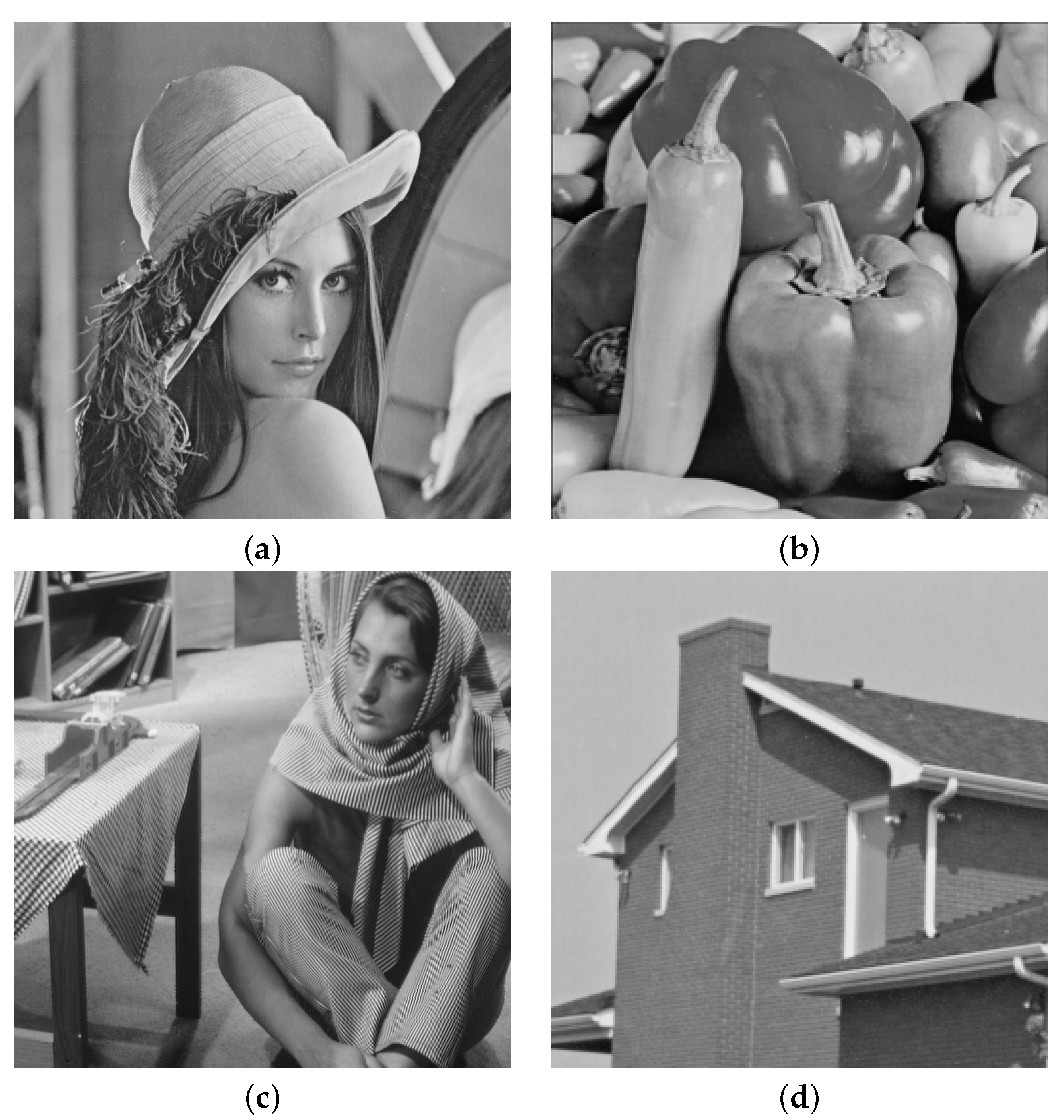
4.1. Experimental Environment

We experimented with our methods by using the images shown in Figure 4. For equivalent comparison, we resized the images to $256\times 256$ pixels and segmented them to $4\times 4$ or $8\times 8$ patches. To measure the performances of different algorithms, we focused on image compression, more specifically, reconstruction with a limited number of coefficients, by comparing PSNR (dB) with the number of used coefficients. Sparse-coding-based algorithms depend on the value of $\lambda$ in their formulations, Equations (3) and (11), because they control the trade-off between the mean square error (MSE) and sparsity. In the compression sense, the optimal value varied from the number of coefficients or bases used in the compression scheme. In this study, we found the value for each target sparsity level via Bayesian optimization with expected implementation and the Màtern 5/2 covariance kernel function. For Bayesian optimization, we used the ’bayesopt’ library offered by MATLAB. For equivalent comparisons, all experiments were implemented using MATLAB R2021a in Windows 10 Education, equipped with an Intel i7-9700 CPU with 32 GB RAM.

All the algorithms used in these experiments are conducted with the same stopping condition. We set the stopping condition to the difference of objective functions between the present and 10 past iterations.

4.2. Comparison with Sparse Orthonormal Transform

This subsection compares the SOT and the proposed method with different numbers of dictionaries for energy compaction. Figure 5 and Figure 6 compare the objective qualities in PSNR (dB) for each number of retained bases. As shown in Figure 5 and Figure 6, our method outperformed SOT (constructed by one orthonormal dictionary) in PSNR (dB). We concluded that this result is due to two reasons: (a) Sparse coding algorithms work better based on the input data classified according to their structure than whole unstructured input data, and (b) the dictionary from a small dataset is more adaptive and more representative than that from a large dataset. Furthermore, the difference in reconstruction errors between the proposed method and the SOT in Figure 6 is less than the difference in Figure 5. Small patches have simpler and more dominant directional information than large patches, whereas large patches usually are more complex and have diverse orientations, leading to the difference. In the next section, we verify whether analysis (a) is correct.

4.3. Effect of Proposed Classification Method

Figure 7 and Figure 8 show that assertion (a) is reasonable. We verified that our proposed classification method for input data by using Equation (4) works well. Figure 7 and Figure 8 show the difference between the two classification methods for different patch sizes. We compared our classification method based on Equation (4) with simply grouping the data evenly in order. In the figures, cls-direction indicates our classification method by using a direction in patch, whereas cls-order indicates a sequentially grouping way. In all cases, our method performs better. In both cases, the use of a larger number of dictionaries increases the PSNR (dB), but for cls-order, the difference is small or negligible. This result indicates that the dictionaries from data grouped by similar structures are more representative than those grouped from irregular and unstructured data.

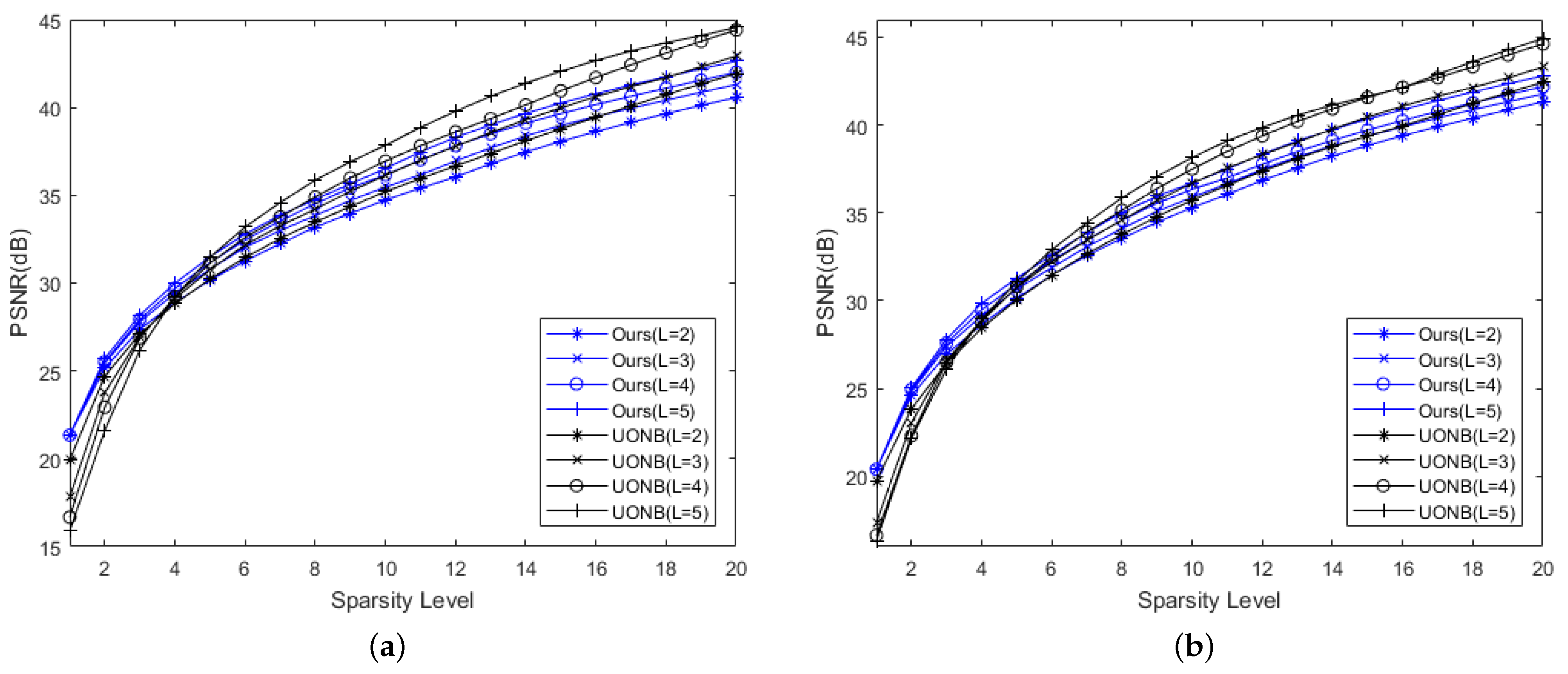
4.4. Comparison with an Overcomplete Dictionary

For a comparison of the proposed method with the overcomplete dictionary-based algorithm, we used a UONB with optimization [10] and block coordinate relaxation algorithm, which is faster than the orthogonal matching pursuit. We performed the experiment using different numbers of dictionaries of the proposed method and UONB, from two to five. Figure 9 and Figure 10 show the differences between our method and UONB. In these figures, the proposed method shows a more powerful performance for small patches. In $8\times 8$ cases, the performance graphs of UONB and the proposed method have crossing points at approximately four retained coefficients. In contrast to UONB, our method exhibits superior performance with an increasing number of dictionaries. In the $8\times 8$ case, our method outperformed UONB with a small number of coefficients, and UONB showed better performance when using a large number of coefficients. In contrast, the proposed method generally performed better than UONB in the $4\times 4$ case. The proposed method also performed better with a small patch size. The UONB performed better in the case of more complex patches with large sparsity levels and a large number of dictionaries. For UONB, a large number of orthonormal dictionaries indicated a wider overcomplete dictionary and involved more redundant and expressive representations. Figure 10 illustrates the results at a high sparsity.

4.5. Processing Time

To reduce the computational time, we attempted to make the best use of the DCT matrix.

Table 1. The processing time and number of iterations for each method. L indicates the number of orthogonal dictionaries. We compare each algorithm with the optimal $\lambda$ value for two different numbers of retained coefficients. The bold texts indicate minimum results.

L	# of Retained Coefficients	SOT		UONB		Proposed
		Iterations	Time (s)	Iterations	Time (s)	Iterations	Time (s)
1	3	2095	1.4553	-	-	-	-
	5	2741	1.9480	-	-	-	-
2	3	-	-	622	49.7882	72	0.0498
	5	-	-	536	82.9780	107	0.0650
3	3	-	-	628	343.3251	183	0.1174
	5	-	-	505	97.5815	157	0.0872
4	3	-	-	482	57.8052	195	0.0920
	5	-	-	754	101.3284	192	0.1007

compares the SOT, UONB, and the proposed method in terms of the number of iterations and the computational time (seconds) until convergence. We performed experiments on UONB and the proposed method for three dictionary sizes: L = 2, 3, and 4. Since the SOT uses only an orthogonal dictionary, it is marked only for L = 1. To design an equivalent experimental setting, we set $\lambda$ values that were optimal to two levels of sparsity: 3 and 5. The time to search $\lambda$ was not considered.

Table 1 shows that our proposed method performed the best in all cases. SOT works better than UONB in terms of computational time. Although the number of iterations required for convergence for SOT was much larger than that required for UONB, SOT was much faster than UONB, because it did not use greedy algorithms. The number of iterations for our proposed method was several times smaller than that for UONB. The degree of reduction varied by approximately two to four times; however, in all cases, our algorithm required fewer iterations. The differences between the computational times was larger than that between the number of iterations. Since our method required fewer iterations and shorter computation time for each iteration than those of UONB, our method was, on average, hundreds of times faster than UONB.

One interesting point is the comparison between SOT and the proposed method. Although the proposed method attempted to find more dictionaries and coefficients than the SOT did, the number of iterations could be reduced by factorizing a dictionary into the DCT matrix and an orthonormal matrix, which prevented an increase in time.

4.6. Effects on a Bayesian Optimization

The Bayesian optimization method was compared with an exhaustive method. We conducted experiments on different image patch sizes and then compared each method by varying the number of iterations.

Table 2. Comparisons of the PSNR(dB) and best $\lambda$ between the Bayesian method and exhaustive method.

		Methods	Bayesian Method		Exhaustive Method
		Iterations	10	30	100	1000
Barbara	4 × 4	PSNR(dB)	31.7748	31.8543	31.8395	31.8545
		$\lambda$	0.0396964	0.040544	0.0200	0.0140
	8 × 8	PSNR(dB)	27.01254	27.1991	25.1582	27.1911
		$\lambda$	0.13714	0.063292	0.0070	0.1330
House	4 × 4	PSNR(dB)	35.5931	35.6488	35.6092	35.6709
		$\lambda$	0.041138	0.026825	0.0200	0.0150
	8 × 8	PSNR(dB)	30.3563	30.3577	30.3283	30.3559
		$\lambda$	0.319391	0.099313	0.1600	0.0980
Lena	4 × 4	PSNR(dB)	32.9539	33.0129	32.9817	33.0218
		$\lambda$	0.051326	0.034557	0.0400	0.0320
	8 × 8	PSNR(dB)	27.7297	27.8073	27.7918	27.8325
		$\lambda$	0.16529	0.069484	0.1400	0.0940
Peppers	4 × 4	PSNR(dB)	33.1043	33.1161	33.0836	33.1197
		$\lambda$	0.046513	0.06335	0.0500	0.0350
	8 × 8	PSNR(dB)	27.3874	27.4054	27.3951	27.4300
		$\lambda$	0.2068	0.21706	0.1900	0.2050

shows the PSNR(dB) for each experiment and the corresponding $\lambda$. We conducted all experiments with $\lambda$ in the range of 0 to 1. We also performed the exhaustive methods for two different strides: 1/100 and 1/1000. The optimal $\lambda$ values from the two methods were either similar or different, but the PSNR(dB)s were generally similar. This result indicated that the proposed method with Bayesian optimization performed similar to the exhaustive method but with a much lower number of iterations.

5. Conclusions

In this paper, we proposed a novel sparse-coding-based image transform framework as an extension of the SOT for efficient implementation. Overcomplete-dictionary-based methods perform well in terms of sparse representation but require a long time and many resources because of their iterative or greedy optimizations. Moreover, they are suitable for image compression as compared to analytic transforms. Orthogonal sparse coding is similar to analytic transforms such as DCT and KLT. Since the dictionary is square and orthonormal, the transform is invertible and conserves the energy of the data. Thus, orthogonal sparse coding-based transforms for image compression have been proposed over the past few decades.

One of these transforms is the SOT. It has been theoretically proven that the SOT outperforms KLT [4]. We extended the SOT based on the unions of several orthonormal dictionaries. Although the number of variables to be computed increased, we prevented the increase in computational time by making the best use of the DCT matrix for the classification of input data and factorization of dictionaries. Consequently, the proposed method outperformed the SOT with a reduction in the computation time. The proposed method satisfies the object of this study through PSNR graphs and a table of processing time. For a more practical implementation, we proposed a scheme to search for the optimal $\lambda$ via Bayesian optimization. Reconstructing an image using a specified number of coefficients was important. Since the performance varied with $\lambda$, determining the optimal value was important. The proposed Bayesian-optimization-based method required fewer iterations than the exhaustive method did.

References

1. Zhang, Z.; Xu, Y.; Yang, J.; Li, X.; Zhang, D. A Survey of Sparse Representation: Algorithms and Applications. IEEE Access 2015, 3, 490–530. [Google Scholar] [CrossRef]
2. Aharon, M.; Elad, M.; Bruckstein, A. K-SVD: An algorithm for designing overcomplete dictionaries for sparse representation. IEEE Trans. Signal Process. 2006, 54, 4311–4322. [Google Scholar] [CrossRef]
3. Elad, M.; Aharon, M. Image Denoising Via Sparse and Redundant Representations Over Learned Dictionaries. IEEE Trans. Image Process. 2006, 15, 3736–3745. [Google Scholar] [CrossRef]
4. Sezer, O.G.; Guleryuz, O.G.; Altunbasak, Y. Approximation and Compression With Sparse Orthonormal Transforms. IEEE Trans. Image Process. 2015, 24, 2328–2343. [Google Scholar] [CrossRef]
5. Kalluri, M.; Jiang, M.; Ling, N.; Zheng, J.; Zhang, P. Adaptive RD Optimal Sparse Coding With Quantization for Image Compression. IEEE Trans. Multimed. 2019, 21, 39–50. [Google Scholar] [CrossRef]
6. Ravishankar, S.; Bresler, Y. Learning Sparsifying Transforms. IEEE Trans. Signal Process. 2013, 61, 1072–1086. [Google Scholar] [CrossRef]
7. Ravishankar, S.; Bresler, Y. Learning overcomplete sparsifying transforms for signal processing. In Proceedings of the 2013 IEEE International Conference on Acoustics, Speech and Signal Processing, Vancouver, BC, Canada, 26–31 May 2013; pp. 3088–3092. [Google Scholar] [CrossRef]
8. Rusu, C.; Thompson, J. Learning fast sparsifying overcomplete dictionaries. In Proceedings of the 2017 25th European Signal Processing Conference (EUSIPCO), Kos, Greece, 28 August–2 September 2017; pp. 723–727. [Google Scholar] [CrossRef] [Green Version]
9. Sezer, O.G.; Harmanci, O.; Guleryuz, O.G. Sparse orthonormal transforms for image compression. In Proceedings of the 2008 15th IEEE International Conference on Image Processing, San Diego, CA, USA, 12–15 October 2008; pp. 149–152. [Google Scholar] [CrossRef]
10. Lesage, S.; Gribonval, R.; Bimbot, F.; Benaroya, L. Learning unions of orthonormal bases with thresholded singular value decomposition. In Proceedings of the IEEE International Conference on Acoustics, Speech, and Signal Processing (ICASSP ’05), Philadelphia, PA, USA, 23 March 2005; Volume 5, pp. v/293–v/296. [Google Scholar] [CrossRef] [Green Version]
11. Shen, B.; Sethi, I.K. Direct feature extraction from compressed images. In Storage and Retrieval for Still Image and Video Databases IV; Sethi, I.K., Jain, R.C., Eds.; International Society for Optics and Photonics, SPIE: Bellingham, WA, USA, 1996; Volume 2670, pp. 404–414. [Google Scholar] [CrossRef] [Green Version]
12. Lee, G.; Choe, Y. Fast and Efficient Union of Sparse Orthonormal Transform for Image Compression. In Proceedings of the 18th International Conference on Signal Processing and Multimedia Applications, SIGMAP 2021, Online Streaming, 6–8 July 2021; Santini, S., Sung, A.H., Eds.; SCITEPRESS: Milano, Italy, 2021; pp. 95–102. [Google Scholar] [CrossRef]
13. Snoek, J.; Larochelle, H.; Adams, R.P. Practical Bayesian Optimization of Machine Learning Algorithms. In Advances in Neural Information Processing Systems; Pereira, F., Burges, C.J.C., Bottou, L., Weinberger, K.Q., Eds.; Curran Associates, Inc.: Red Hook, NY, USA, 2012; Volume 25. [Google Scholar]
14. Frazier, P.I. A Tutorial on Bayesian Optimization. arXiv 2018, arXiv:1807.02811. [Google Scholar]
15. Rubinstein, R.; Zibulevsky, M.; Elad, M. Double Sparsity: Learning Sparse Dictionaries for Sparse Signal Approximation. IEEE Trans. Signal Process. 2010, 58, 1553–1564. [Google Scholar] [CrossRef]
16. Boyd, S.; Parikh, N.; Chu, E.; Peleato, B.; Eckstein, J. Distributed Optimization and Statistical Learning via the Alternating Direction Method of Multipliers. Found. Trends® Mach. Learn. 2011, 3, 1–122. [Google Scholar] [CrossRef]
17. Yang, J.; Zhang, Y. Alternating Direction Algorithms for L1-Problems in Compressive Sensing. SIAM J. Sci. Comput. 2011, 33, 250–278. [Google Scholar] [CrossRef]
18. Schütze, H.; Barth, E.; Martinetz, T. Learning Efficient Data Representations with Orthogonal Sparse Coding. IEEE Trans. Comput. Imaging 2016, 2, 177–189. [Google Scholar] [CrossRef]
19. Rusu, C.; Dumitrescu, B. Block orthonormal overcomplete dictionary learning. In Proceedings of the 21st European Signal Processing Conference (EUSIPCO 2013), Marrakech, Morocco, 9–13 September 2013; pp. 1–5. [Google Scholar]
20. Bao, C.; Cai, J.F.; Ji, H. Fast Sparsity-Based Orthogonal Dictionary Learning for Image Restoration. In Proceedings of the 2013 IEEE International Conference on Computer Vision, Sydney, Australia, 1–8 December 2013; pp. 3384–3391. [Google Scholar] [CrossRef]
Figure 1. The basis of two-dimensional discrete cosine transform. Each basis includes horizontal or vertical directional information.
Applsci 12 02421 g001
Figure 2. PSNR(dB) for different values of λ . This resulted from the case of three orthonormal dictionaries and target sparsity 3.
Applsci 12 02421 g002
Figure 3. The objective function of Bayesian optimization for λ in Figure 2.
Applsci 12 02421 g003
Figure 4. Test images. We experiment with and verify the proposed method with four images. (a) Lena, (b) peppers, (c) Barbara, (d) house.
Applsci 12 02421 g004
Figure 5. The object quality comparison: PSNR (dB) versus the number of retained coefficients for 4 × 4 patches between SOT and our methods. (a) Lena, (b) peppers, (c) Barbara, (d) house.
Applsci 12 02421 g005
Figure 6. The object quality comparison: PSNR (dB) versus the number of retained coefficients for 8 × 8 patches between SOT and our methods. (a) Lena, (b) peppers, (c) Barbara, (d) house.
Applsci 12 02421 g006aApplsci 12 02421 g006b
Figure 7. The object quality comparison: PSNR (dB) versus the number of retained coefficients for 4 × 4 patches between classification methods with different numbers of orthogonal dictionaries. (a) Lena, (b) peppers, (c) Barbara, (d) house.
Applsci 12 02421 g007
Figure 8. The object quality comparison: PSNR (dB) versus the number of retained coefficients for 8 × 8 patches between classification methods with different numbers of orthogonal dictionaries. (a) Lena, (b) peppers, (c) Barbara, (d) house.
Applsci 12 02421 g008
Figure 9. The object quality comparison: PSNR (dB) versus the number of retained coefficients for 4 × 4 different patch sizes between UONB and our methods with different numbers of orthogonal dictionaries. (a) Lena, (b) peppers, (c) Barbara, (d) house.
Applsci 12 02421 g009
Figure 10. The object quality comparison: PSNR (dB) versus the number of retained coefficients for 8 × 8 different patch sizes between UONB and our methods with different numbers of orthogonal dictionaries. (a) Lena, (b) peppers, (c) Barbara, (d) house.
Applsci 12 02421 g010aApplsci 12 02421 g010b