Artificial Intelligence (AI)-Based Evaluation of Bolt Loosening Using Vibro-Acoustic Modulation (VAM) Features from a Combination of Simulation and Experiments

Abstract

The detection of bolt loosening using vibro-acoustic modulation (VAM) has been increasingly investigated in the past decade. However, conventional nonlinear coefficients, derived from theoretical analysis, are usually based on the assumption of ideal wave–surface interactions at the joint interfaces. Such coefficients show a poor correlation with the tightening torque when the joint is under the combined influences of structural and material nonlinearities. A reliable inspection method of residual bolt torque is proposed in this study using support vector regression (SVR) with acoustic features from VAM. By considering the material intrinsic nonlinearity (MIN) and dissipative nonlinearity (DN), the responses of aluminum–aluminum and composite–composite bolted joints during the VAM test were accurately simulated. The SVRs were subsequently established based on the database built by combining simulated and experimental nonlinear spectral features when the joints were inspected at different scenarios. The results show that the evaluation of residual torque using the SVR models driven by the acoustic nonlinear responses had higher accuracy compared to the conventional nonlinear coefficients. Requiring limited experimental data, the proposed method can achieve a reliable inspection of bolt torque by including the simulated data in the machine training.

1. Introduction

Bolted joints are widely used in engineering assets, transferring loads between connected structures. However, an axial preload of the bolts will inevitably decrease during their long-term service, which would increase the possibility of structural failure. Hence, monitoring the residual preload of bolts is of great significance to ensure the mechanical performance of structures.

Over the past decades, increasing efforts have been directed to develop non-destructive testing and evaluation (NDT&E) and structural health monitoring (SHM) methods for damage characterization of bolted structures. Among them, ultrasonic testing (UT) is one of the most commonly used techniques for the evaluation of bolt loosening [1]. Conventional UT is conducted to assess the stress conditions of bolts based on the changes in the linear ultrasonic features (e.g., energy attenuation [2], velocity [3]). However, the linear signal features, which are mainly affected by the global material properties, may not be remarkable when local damage or deterioration occurs [4,5].

Recently, some researchers [6,7] have found that nonlinear acoustic features, generated by the contact acoustic nonlinearity (CAN) at structural interfaces (e.g., cracks and contact surfaces) have higher sensitivity to structural damage compared to the linear ultrasonic features. The nonlinear signal components, such as second-order harmonics (SOHs) [8] and subharmonics [9], induced by CAN are widely applied to detect bolt loosening. However, the above-mentioned nonlinear features consist of a great proportion of nonlinear components (e.g., SOH) [10,11] generated by the inspection system, when a single excitation is used in the inspection. Additionally, a single transducer can hardly provide enough information for the damage state in practical applications [12]. In order to enhance the inspection accuracy against the noises from instruments, vibro-acoustic modulation (VAM) has attracted increasing attention for SHM and NDT&E. The VAM technique adopts two excitation signals, namely a low-frequency (LF) pumping wave and a high-frequency (HF) probing wave. Nonlinear signal features are extracted at the frequencies and are the difference and sum of the frequencies of the two excitations. Therefore, a relatively low level of measurement noise is involved in the VAM test and, consequently, the nonlinear responses in signal spectra [13] (i.e., sidebands (SBs)) can be quantitatively correlated to the health condition of the inspected structure. Zhang et al. [4] proposed a monitoring method of bolt loosening in both composites and metallic joints using nonlinear sideband features, regardless of their working conditions. Considering the local material characters at the contact surface, Zhang et al. [13] developed a finite element (FE) model consisting of two Euler–Bernoulli beam components with two degrees of freedom (DOFs) to accurately predict the VAM responses of the bolted joints. To further improve the practical applicability of this method, Wang et al. [14] applied a piezoceramic transducer, smaller than the conventional shaker, to excite the LF pumping wave and combined the linear swept and time reversal technique in the bolted joint to enhance the signal intensity of nonlinear features. In addition, Wang and Song [15] proposed a novel method based on the Gnome entropy gEn and random forest to detect multi-bolt loosening.

Even though many applications of nonlinear features in damage evaluation using the VAM technique have been conducted, the diverse nonlinear modulation mechanisms are still not clearly understood [16]. Some researchers [16,17,18,19] have reported that the generation of nonlinear structural acoustic features may be a combined result of several different mechanisms besides CAN, such as dissipative nonlinearity (DN) and material intrinsic nonlinearity (MIN). Hence, the existing evaluations of bolt loosening using the nonlinear coefficients established by the CAN model are confronted with the following obstacles:

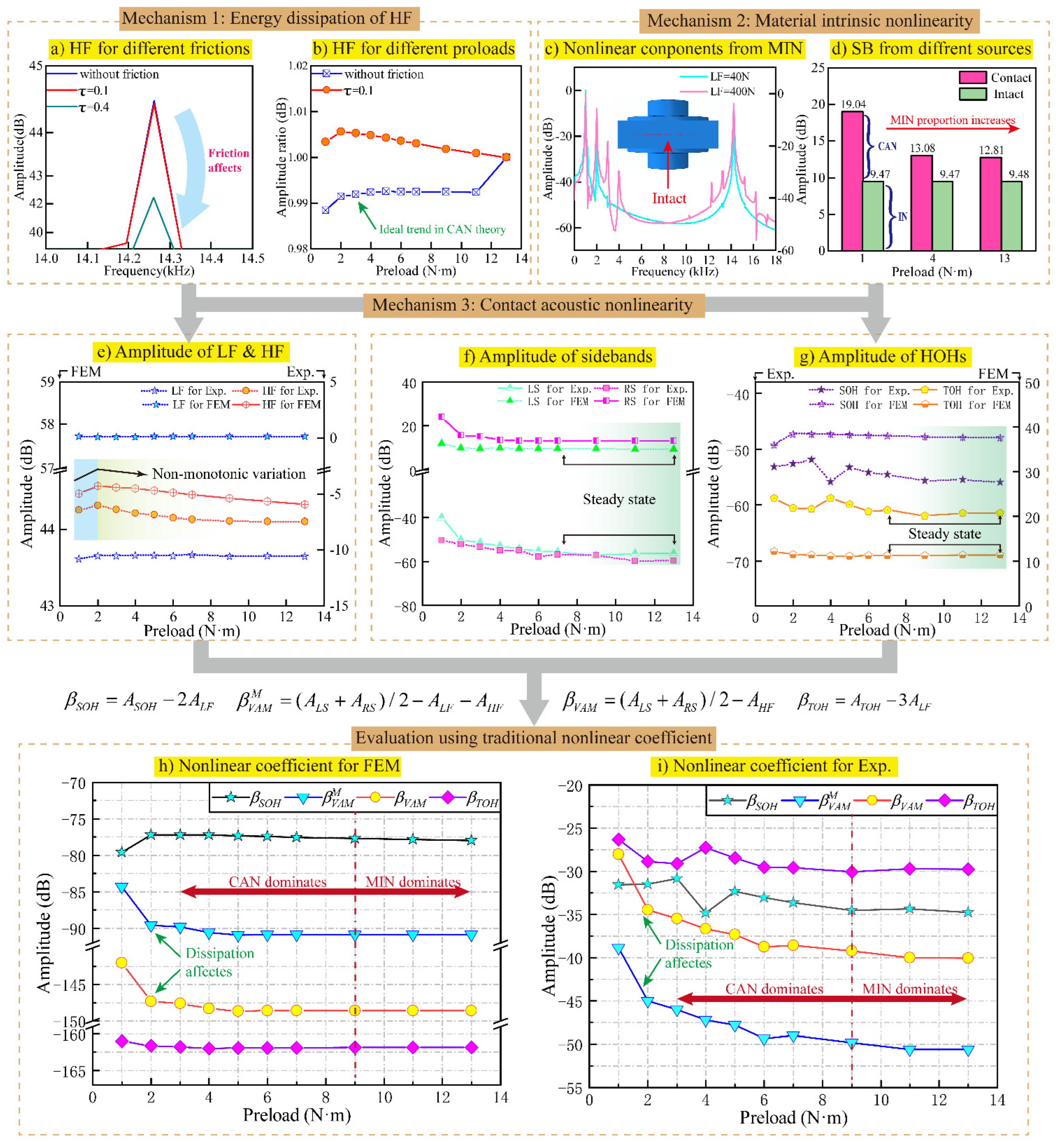
• The nonlinear coefficients are defined using the amplitudes of the spectral linear and nonlinear components. Consequently, such coefficients may vary inconsistently with the theoretical trend for the CAN model when the amplitudes are affected by the other nonlinear sources.
• The above-mentioned potential nonlinearities and CAN are always affected by the same factors (e.g., contact, temperature, and friction). So, it is challenging to quantitatively decouple the interferences of different mechanisms by controlling the experimental conditions [20].
• Proposing a new theoretical damage index by considering the combined influences of the diverse nonlinear mechanisms needs more effort for accurate modeling.

In this paper, the combined influences of multi-nonlinearities in VAM are analyzed and an alternative method using machine learning is proposed to improve the prediction accuracy of bolt loosening of both metallic and composite bolted joints. In Section 2, the major nonlinear mechanisms existing in bolted joints are discussed. Then, the finite element model and experimental setup are detailed in Section 3. As a result, the nonlinear responses of VAM in the bolted joint are shown in Section 4, and the combined influences of the different nonlinearities on the inspection efficiency are discussed in Section 5. Finally, in Section 6, the SVR method, driven by the FE and experimental data, is used to evaluate the preload of aluminum–aluminum and composite–composite bolted joints.

2. Theoretical Background

In order to comprehensively understand the nonlinear responses of bolted joints under different torques, the interfacial contact acoustic nonlinearity, material dissipative nonlinearity and material nonlinearity were considered in this work.

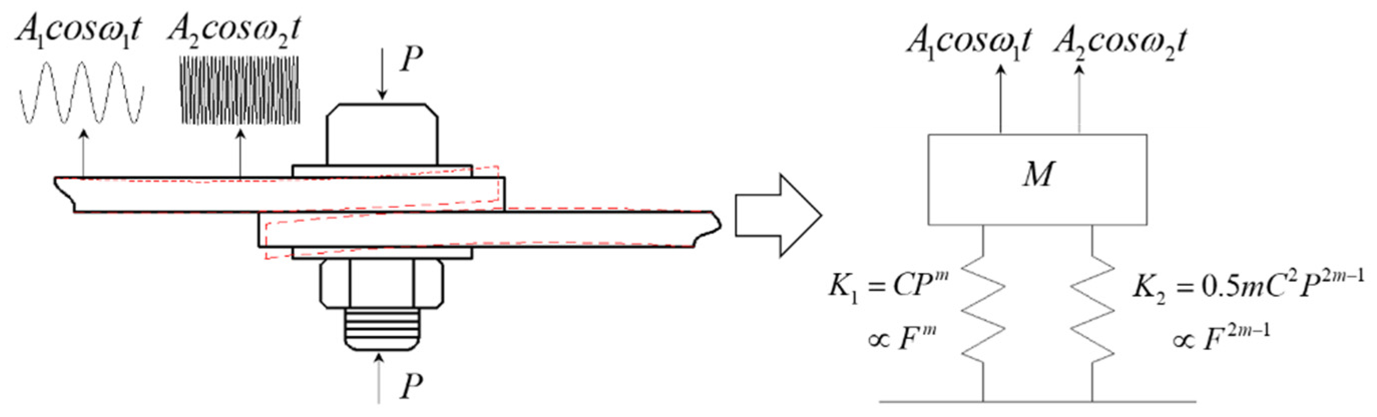
2.1. Contact Acoustic Nonlinearity

The nonlinear acoustic responses generated by CAN are always stronger than those resulting from the other nonlinearities [18], and thus, the nonlinear coefficients derived from the CAN model are widely used as the damage indices of SHM and NDT&E.

In a bolted joint, the preload F induced by the applied torque T can be described by

$$F=T/\left(\tau d\right),$$

(1)

where τ is the friction coefficient between the bolt and nut, and d is the diameter of the bolt.

In the VAM-based method, the loose joint is subjected to mixed excitation from a low-frequency pumping vibration (with an equivalent force A₁cosω₁t) and a high-frequency probing wave (with an equivalent force A₂cosω₂t), which are independent of each other, as exhibited in Figure 1.

When the motion of the bolted interfaces excited by the two waves conforms to the “opening–closing” behavior in the CAN model, the relationship between the contact stiffness and the applied load is suggested to be [21]:

$$K_1=C{p}^m\propto F^m\propto T^m,$$

(2)

$$K_2=0.5m{C}^2{p}^{2m-1}\propto F^{2m-1}\propto T^{2m-1},$$

(3)

where p is the contact pressure, K₁ is the linear stiffness, and K₂ is the nonlinear stiffness of the contact interface. C and m are associated with the surface properties of the material in contact.

The equation of the motion of the joint can be described as:

$$M\ddot{x}+K_{1}x-\varphi K_2{x}^2=A_1\cos {\omega }_{1}t+A_2\cos {\omega }_{2}t,$$

(4)

where ω₁ and ω₂ are the frequencies of the pumping vibration and probing wave, respectively, and ϕ is a small quantity to scale the perturbation to be minute.

To solve Equation (4), the analogous method based on perturbation theory is used, and the second-order nonlinearity of the solution is considered. The details of the derivation of this solution are presented in [4,22]. As a result, we can have x in the form of a combined wave, including the fundamental waves at ω₁ and ω₂, the SOHs at 2ω₁ and 2ω₂, the three-order harmonics (TOHs) at 3ω₁ and 3ω₂, and the SBs, viz., the right sideband (RS) at ω₁ + ω₂ and the left sideband (LS) at ω₁ − ω₂. The amplitudes of the signal components satisfy the relations

$$A_{SOH}=\frac{0.5K_2}{K_1-4M{\omega }_1{}^2}{A}_{LF}^2,$$

(5)

$$A_{TOH}=\frac{0.5K_2^2}{(K_1-9M{\omega }_1{}^2)(K_1-4M{\omega }_1{}^2)}{A}_{LF}^3,$$

(6)

$$A_{SB}=\frac{K_2^{}}{K_1-M{({\omega }_1\pm {\omega }_2)}^2}{A}_{LF}^{}{A}_{HF}^{}.$$

(7)

Then, the nonlinear coefficients β can be defined in the unit of dB as

$${\beta }_{SOH}=A_{SOH}-2A_{LF},$$

(8)

$${\beta }_{TOH}=A_{TOH}-3A_{LF},$$

(9)

$${\beta }_{VAM}^M=(A_{LS}+A_{RS})/2-A_{LF}-A_{HF},$$

(10)

$${\beta }_{VAM}=(A_{LS}+A_{RS})/2-A_{HF}.$$

(11)

By eliminating the linear terms (i.e., LF and HF), the nonlinear coefficients β only depend on the contact stiffness K₁ and K₂ and are related to the preload F and torque T. According to CAN theory, the nonlinear coefficients decrease with the increase in the preload (i.e., the applied torque).

2.2. Dissipative Nonlinearity

The latest experiments have shown that nonlinear energy dissipation can be caused in the structure at the mesoscopic interfaces (such as cracks or contact surfaces) in the case of VAM [16,18,23,24]. The most significant phenomenon of such dissipation is the HF wave dampened by a stronger LF wave.

Moreover, dissipative nonlinearity (DN) was indicated to occur either in a low-strain level crack surface perturbation (e.g., thermal [25]) or a relatively highly intense interaction (e.g., friction [26] or hysteresis [27]). However, differentiation between the two dominant dissipation mechanisms is usually difficult to obtain in practice [20]. Assuming that the structural nonlinear responses are dominated by thermo-elastic dissipation, the HF losses at the inner contact of the cracks can be described as [28]

$$W_{HF}^{dis}=\left(\frac{2\pi }{{\omega }_L}\right)\kappa \eta {\left(\frac{\alpha E}{H\rho }\right)}^2\overline{L}{\left(\frac{L}{l}\right)}^2{\epsilon }^2,$$

(12)

where η is the temperature, α is the temperature expansion coefficient of the solid, E is the bulk elastic modulus, ρ is the density, H is the specific heat, ε is the average strain, κ is the thermal conductivity, and ω_L is the relaxation frequency for the defect scale L. Recently, Qin et al. [16] revealed that the dissipation based on the thermo-elastic coupling may be more efficient in the bolted joint; meanwhile, frictional and adhesional hysteretic dissipation may also exist. The contribution of the dissipation mechanism may cause continuous effects on the spectral amplitudes in VAM testing, which cannot be neglected.

2.3. Material Intrinsic Nonlinearity

In this article, material intrinsic nonlinearity specifically refers to the global material nonlinearity (i.e., classical nonlinearity), which differs from the instrumental nonlinearity and the local Hertzian nonlinearity. The MIN theory is based on a high-order expansion of the classical Hooke’s law, and the MIN is determined by the material atomic properties (e.g., Lame constants) and is able to introduce the nonlinear features without interfaces.

Hooke’s law is based on the second-order expansion of free energy in the power series as [18]:

$$G=G_0+\frac{1}{2}\lambda u_{\mathrm{ii}}^2+\mu u_{\mathrm{i}k}^2,$$

(13)

where G₀ is the initial value, λ and μ are the Lame constants and u_ik is the deformation tensor, which can be described as:

$$u_{ik}=\frac{1}{2}\left(\frac{\partial u_i}{\partial x_k}+\frac{\partial u_k}{\partial x_i}\right).$$

(14)

Considering a third-order series of u_ik, we have:

$$u_{ik}=\frac{1}{2}\left(\frac{\partial u_i}{\partial x_k}+\frac{\partial u_k}{\partial x_i}+\frac{\partial u_l}{\partial x_i}\frac{\partial u_l}{\partial x_k}\right),$$

(15)

which can cause a nonlinear quadratic waveform (i.e., SOH) in the solution of the motion equation. The SB (at the frequencies of ω₁ ± ω₂) can be generated when LF and its SOH interact due to the intrinsic material nonlinearity.

Even though MIN has been reported as a weaker contribution to structural nonlinear responses, compared to CAN [18,29] in a structure with imperfect interfaces, it is worth noting that MIN still can become a dominant nonlinear source when the CAN is relatively weak (e.g., strongly bonded or tightening interfaces).

3. Finite Element Model and Experiment

Considering the difficulties in separating the different nonlinearities in experiments, a finite element method (FEM) with flexible operability in properties (e.g., material and friction) was adopted to establish a more comprehensive analysis of the influences of nonlinearities on the nonlinear responses.

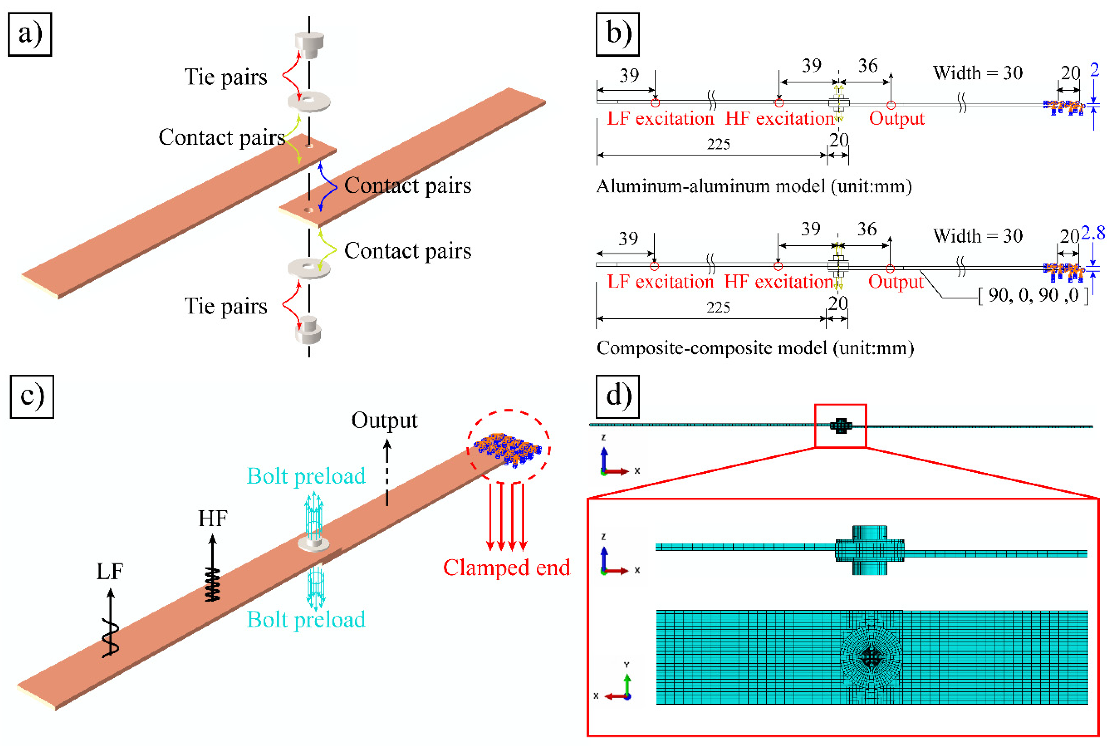
3.1. Finite Element Model

ABAQUS/standard was used to establish the finite element models of bolted joints. The simulation conditions (e.g., material parameters, sizes, boundaries, loads, and excitations) were set to be the same as the experimental conditions.

Each model consisted of two beams connected by an M6 bolt and two washers (Figure 2a). The interactions between the beam–beam pairs and washer–beam pairs were defined as normal hard contact with penalty friction for contact, and the bolt–washer pairs were tied. Aluminum and composite beams were investigated in this work, whose connect modes are denoted as Al–Al and C–C. The geometric and material parameters are shown in

Table 1. Material parameters of the bolted joints.

Material Type	Elasticity Modulus E(GPa)	Poisson’s Ratio ν	Density (kg/m3) ρ	Friction Coefficient τ
Aluminum	75.6	0.33	2700	0.1
Composites	E1/E2/E3	ν11/ν13/ν23	1700	0.2
	130/7/7	0.32/0.32/0.45

and Figure 2b.

The simulation process consisted of two steps, viz., the bolt preload application and VAM propagation (Figure 2c). One end of the beam was clamped to make the whole structure a cantilever. The bolt preload was set as the axial compressive stress applied to the center of its cross-section, whose amount was equivalent to the applied torque in the experiment (calculated by Equation (1)). After the preloading of the bolt, continuous LF and HF sine waves were simultaneously excited at the free beam, and the transmitted waves were detected by an output node at the clamped beam. The excitations were selected by the modal tests to ensure the measurable out-of-plane displacement of the joints. For the Al–Al joints, LF = 0.99 kHz and HF = 14.24 kHz. For the C–C joints, LF = 0.76 kHz and HF = 14.99 kHz. The minimum time step interval was 5μs, and the sampling frequency was 200 kHz. In order to precisely capture the waveform, the grids were meshed to satisfy the minimum requirements, i.e., eight nodes per shortest wavelength [30].

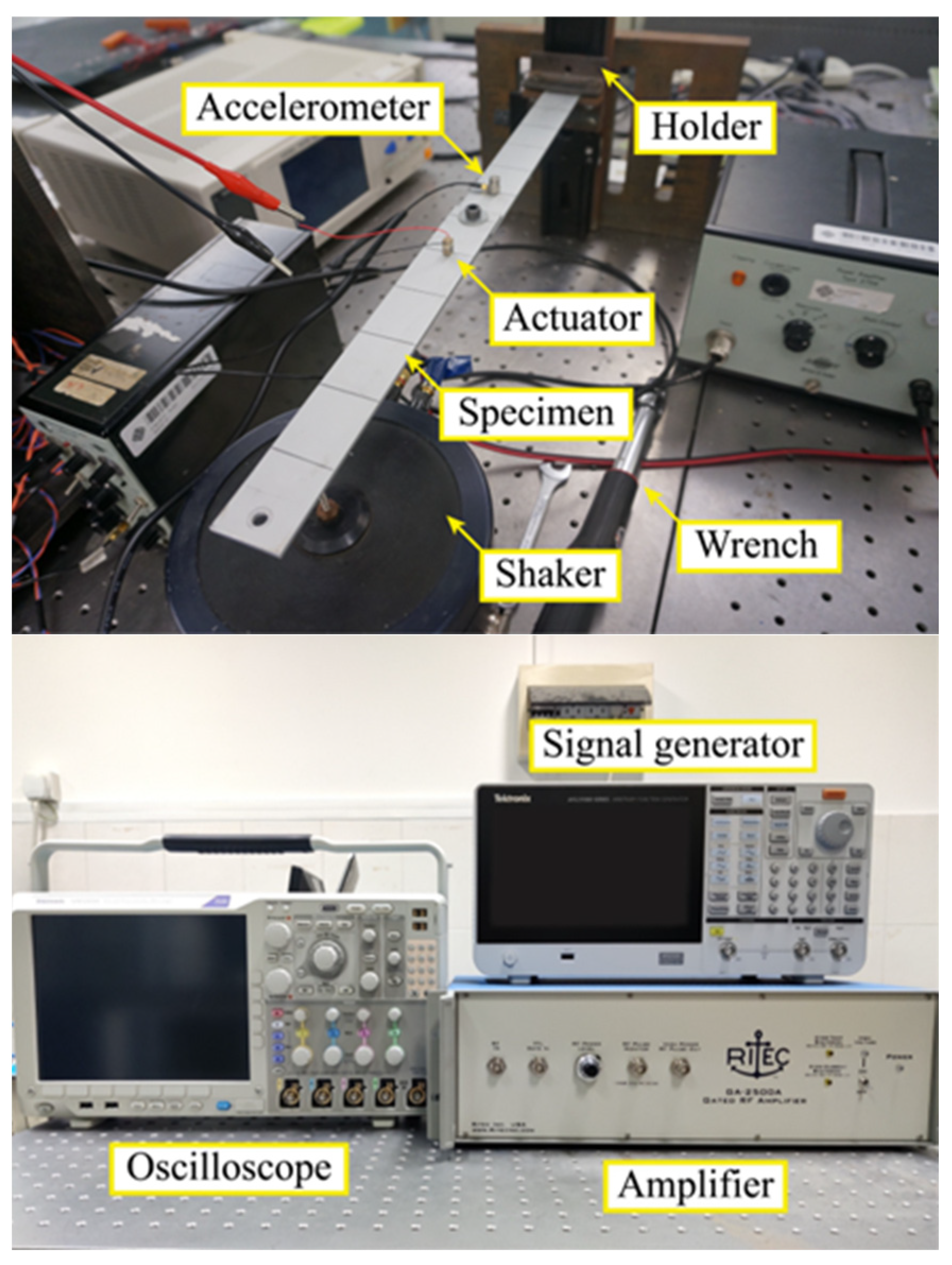
3.2. Experimental Setup

The setup of the experiment is shown in Figure 3. The experimental procedure was as follows: firstly, the specimen was clamped by a holder, and the preload of the bolt was applied by a torque wrench. Next, the LF vibration was excited by a shaker (B&K^®, Model type: 4809, Virum, Denmark). Meanwhile, the HF probing wave was generated by a signal generator (Tektronix^®, AFG 31000, Beaverton, OR, USA) and amplified by an amplifier (Ritec^®, GA-2500A, Warwick, RI, USA) before introducing on the specimen by an actuator (PI^®, P-885.11, Karlsruhe, Germany). Lastly, the response signals of the bolted joints under the mixed excitations were captured with an accelerometer (B&K^®, Model Type: 4393, Virum, Denmark).

4. VAM Responses of Bolted Joints

The VAM responses of the two types of joints are similar in contour and time domain, and hence, only those of the Al–Al bolted joints are presented in this section.

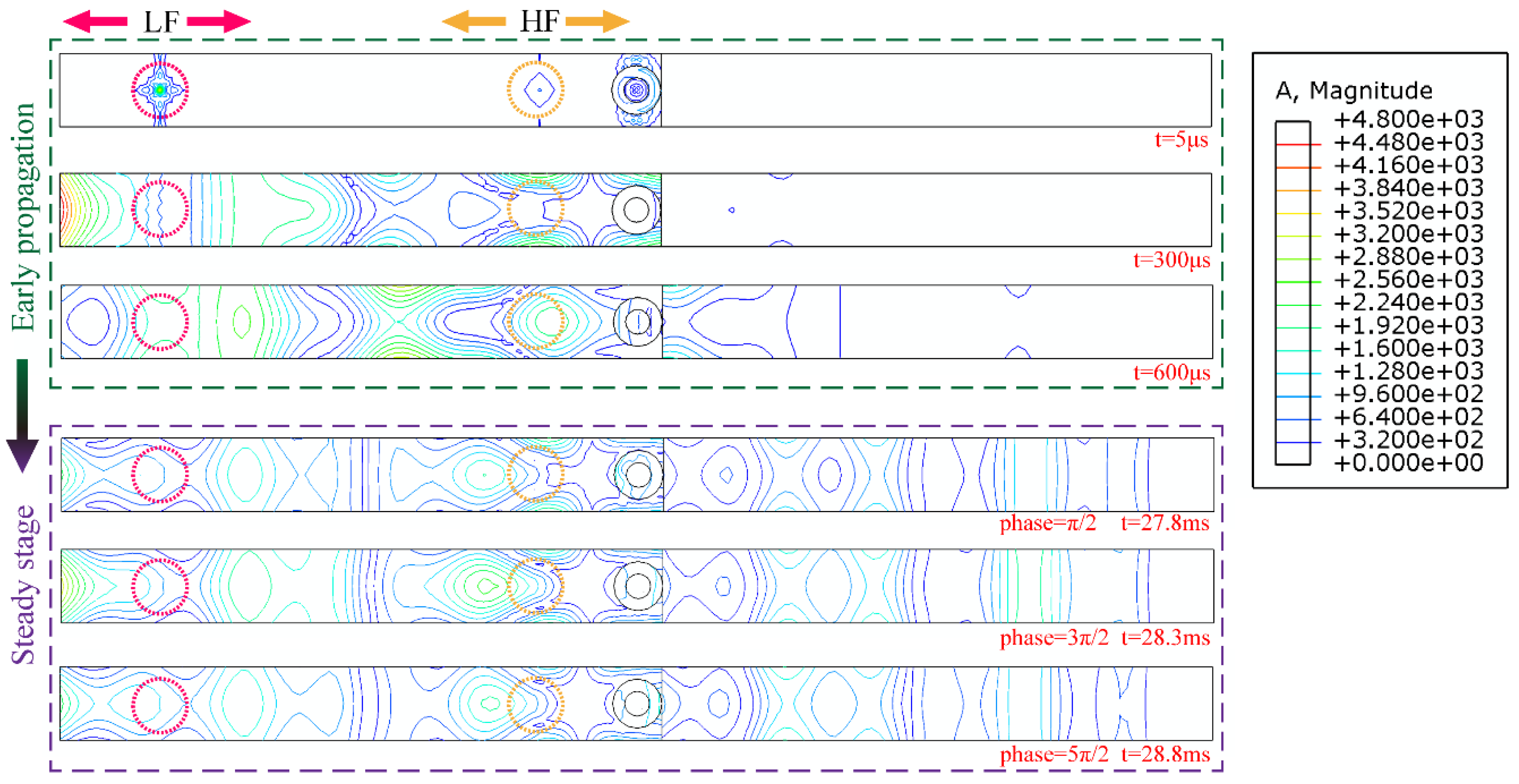
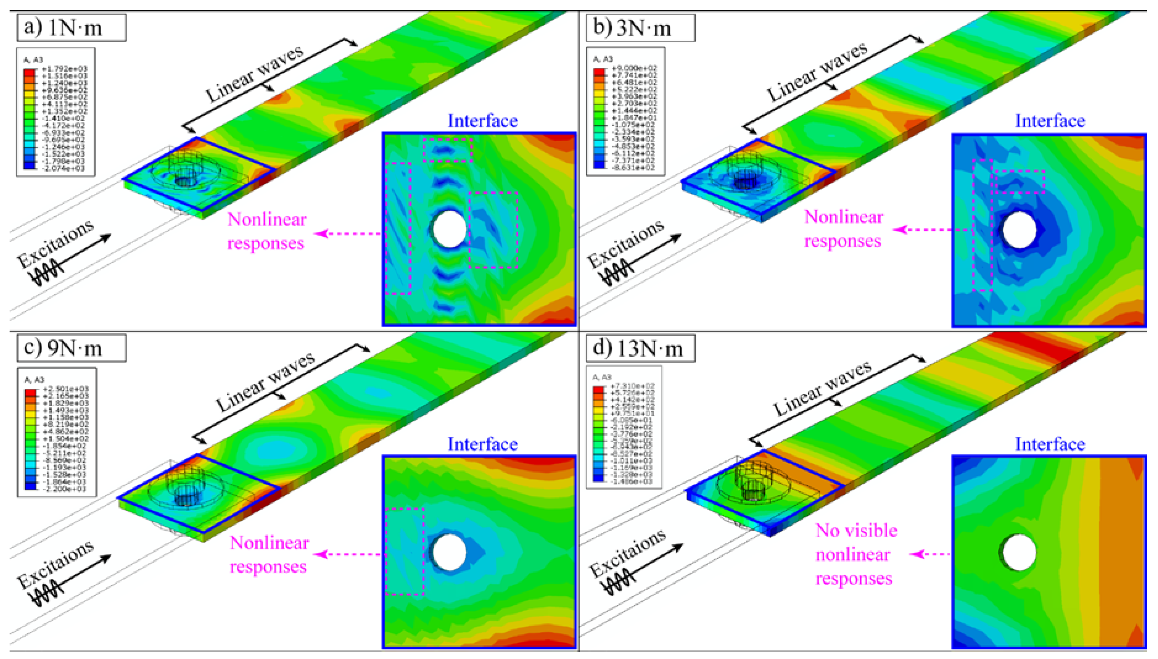
4.1. Acceleration Contour

The steady global wave field is formed during the propagation and interaction of the LF and HF. Figure 4 shows the process of the VAM behavior of the Al–Al bolted joint, which presents an early propagation and a steady stage. Initially, the LF vibration and the HF probing wave appeared at the two excited nodes on the free beam (t = 5 μs), transmitting to the clamped beam along the central contact region near the preloaded bolt before covering the whole structure (t = 600 μs). Next, a steady acceleration contour was formed after a millisecond of reciprocating propagation of the combined waves in the structure. Then, the contours for every 0.5 ms (per half period) were similar to each other due to the energy dominant of the LF pumping vibration (period = 1 ms), and the micro variation was caused by the HF contribution (period = 0.07 ms).

The contours of the out-of-plane acceleration (A3) of the bolted joint at the same time under different preloads are shown in Figure 5. It can be seen clearly that nonlinear waves were generated in the contact region (Figure 5a). The nonlinear responses in the contact region consisted of multiple components with different wavelengths (i.e., different frequencies) and modal shapes. However, the nonlinear responses in the joint diminished with the increase in the preload (Figure 5a–d), because the “opening–closing” motion was obstructed by the enhancement of the contact constraint, while the LF pumping excitation was maintained at the same level. Actually, the nonlinear features can barely be observed from 9 N·m to 13 N·m in the contours.

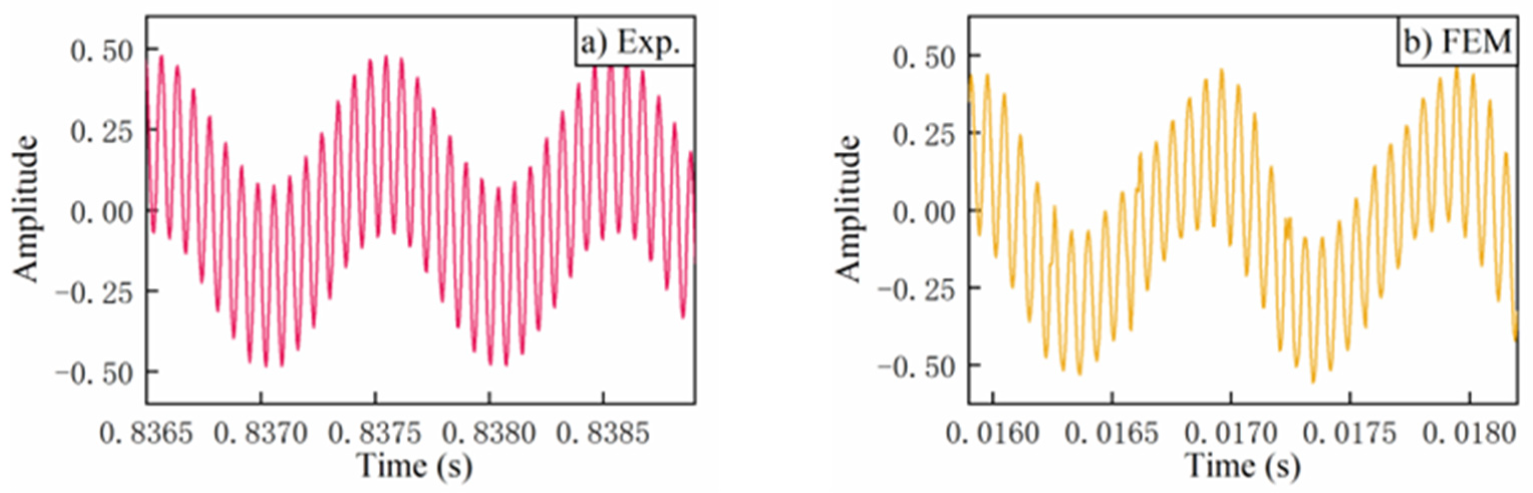
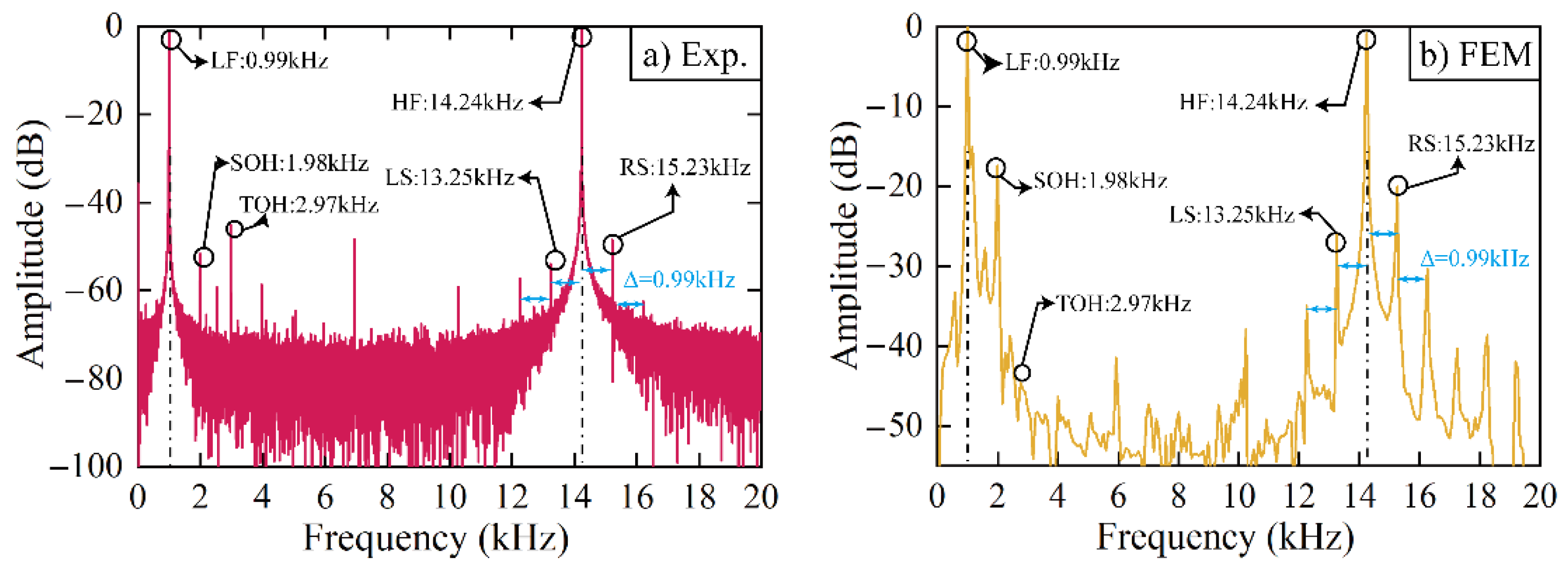
4.2. Collected Signals

The normalized time-domain signals of the FEM and experiment (Figure 6) only showed the two linear frequencies, viz., the LF and HF excitations. The signal characters collected from the FEM and experiment are in a good agreement.

The nonlinear features can be seen in the typical frequency spectra for both the experiment and FEM (Figure 7). The main energy was focused on the linear components (i.e., 0.99 kHz LF and 14.24 kHz HF). The HOHs (i.e., 1.98 kHz SOH and 2.97 kHz TOH) and SBs (13.25 kHz LS and 15.23 kHz RS) also had distinct amplitude peaks.

5. Nonlinear Coefficients of Joints under Different Preloads

The investigation into the nonlinear signals from the joints under different preloads was divided into three aspects. Firstly, the influences of the different nonlinearity contributions, except for CAN (i.e., DN and MIN), were investigated (Figure 8a–d). Next, the signal amplitudes of the joints under different preloads were detected, as shown in Figure 8e–g. Finally, the amplitudes were used to calculate the nonlinear coefficients according to the CAN theory (Equations (8)–(11)). The evaluation results of the bolt preloads using the nonlinear coefficients are shown in Figure 8h,i.

5.1. Influence of Dissipative Nonlinearity

The FEM results in Figure 8a,b indicate that measurable energy dissipation on HF excitation can be caused by the LF vibration in the VAM process. Interface friction is one of the major factors affecting the DN phenomenon [31]. Therefore, interface friction was the focus of this work, considering the actual interface friction may be significantly different due to the manufacturing deviation between different joints. The amplitude at 1 N·m declined with the increase in the friction coefficient τ (Figure 8a). Additionally, a non-monotonic variation in the HF amplitude under different preloads can be seen in Figure 8b, in contrast to the ideal monotonic trend conforming to the CAN model when the friction = 0. This means the HF amplitude can decrease due to individual differences in the joint friction, and the amount of dissipation is different under different preloads.

5.2. Influence of Intrinsic Nonlinearity

In order to reveal the influence of MIN, all of the interfaces of the FE model were tied to make the bolted joint an intact structure (Figure 8c) without any interface. The signal energy was normalized to 0 dB in Figure 8c, and the nonlinear responses (i.e., SOH, LS, and RS) of the intact structure were still measurable, which means the generations of nonlinear responses could be caused not only by the CAN mechanism but also the material intrinsic material nonlinearity. By enhancing the LF pumping vibration to 400 N to enlarge the effect of MIN, the amplitudes of the nonlinear components were much higher than that when LF = 40 N. The dependence of the MIN generations on the vibration amplitude was also reported by Dao et al. [32].

Furthermore, in Figure 8d, the LS amplitudes of the intact and contact models for different preloads are compared. The nonlinear amplitudes (i.e., LS) caused by MIN in the intact model were not sensitive to the changes in the preloads (Figure 8d), while the LS declined with increasing preloads when both the CAN and MIN were considered in the contact model. In other words, the nonlinear amplitudes at the high-stress stages were mainly caused by MIN, while at low-stresses stages, CAN dominated the nonlinear responses.

5.3. Combined Results of Nonlinearities

The dependence of the experimental and simulated amplitudes on the preloads was consistent. In terms of the linear components (Figure 8e), the LF amplitudes stayed at the same level for all stress stages. The HF amplitudes, affected by the nonlinear dissipation, increased slightly under the preload from 1 N·m to 2 N·m and subsequently decreased with the increase in the load. Additionally, the amplitudes of nonlinear components, viz., SOH, TOH, LS, and RS in Figure 8f show measurable reductions with the increase in the preload initially and then stay steady for the high loads (about 9 N·m–13 N·m). As a result (Figure 8h,i), the experimental and FEM nonlinear coefficients generally decreased with the increase in the preload, as predicted by CAN theory. However, the influences of MIN and DN on the nonlinear coefficients were unneglectable. The coefficients related to the HF amplitude took a dive at 2 N·m and were affected by DN. Meanwhile, all the coefficients dominated by MIN remained at a steady stage over 9 N·m, leading to difficulties in the early-stage warning for bolt loosening.

From the above analysis, it is still challenging to quantitatively measure the influences of these combined contributions on the nonlinear responses of a loose bolted joint, even though many efforts have been made by researchers. Hence, a new intelligent method that considers the local influences caused by multi-mechanisms on acoustic nonlinearity generation is needed to make full use of the nonlinear features.

6. Intelligent Evaluation of Bolt Preload Using SVR

The SVR model driven by the spectral amplitudes was chosen to implement the AI-based evaluation of bolt preload in this work for the following reasons:

• A mapping relation can be established between the amplitude and preload according to the results in Section 5. The sample consisting of multiple features (i.e., LF, HF, SOH, TOH, and SBs) can improve the accuracy of the load evaluation even when the joint is under the influences of different nonlinearities.
• SVR is a classical machine learning method and has been well tested in long-term applications. Moreover, a fairly simple model without extensive trials and errors can certify the feasibility of the AI evaluation using the nonlinear features.

6.1. Algorithm

The model between the amplitude vector x_i and preload y_i was established by SVR. The Gaussian radial basis function (RBF) is used as the kernel function y = f(x) to map the vector to a high-dimensional space, and then the regression function y = f(x) is solved to minimize the structural risk.

The regression function f(x) for a training sample $\left\{(x_i,y_i),i=1,2,\dots ,n\right\}$ is

$$f(x)=w·\varphi (x)+b,$$

(16)

where w is the weight coefficient, b is the bias term, and ϕ(x) is the nonlinear mapping.

The v-SVR model is used to minimize loss coefficient ε. In this model, the minimizing equation is equivalent to the optimization problem:

$$\left\{\begin{array}{l}\underset{w,{\xi }_i,{\xi }_i^{\ast },b}{\min }\frac{1}{2}{‖w‖}^2+c\left[v\epsilon +\frac{1}{n}{\displaystyle \sum _{i=1}^n({\xi }_i+{\xi }_i^{\ast })}\right]\\ \mathrm{s}.\mathrm{t}. (w·\varphi (x_i)+b)-y_i\le \epsilon +{\xi }_i\\ y_i-(w·\varphi (x_i)+b)\le \epsilon +{\xi }_i^{\ast }\\ {\xi }_i,{\xi }_i^{\ast }\ge 0,\epsilon \ge 0\end{array}\right.,$$

(17)

where ${\xi }_i,{\xi }_i^{\ast }$ are the relaxation variables, and v is a model parameter used to control the number of support vectors or the number of error samples.

The dual equation of the original optimization problem is derived as Equation (18) on the basis of the Karush–Kuhn–Tucker condition by introducing the Lagrangian multiplier ${\alpha }_i,{\alpha }_i^{\ast }$.

$$\left\{\begin{array}{l}\min {\displaystyle \sum _{i=1}^n({\alpha }_i-{\alpha }_i^{\ast })y_i-\frac{1}{2}{\displaystyle \sum _{i=1}^n{\displaystyle \sum _{j=1}^n({\alpha }_i-{\alpha }_i^{\ast })({\alpha }_j-{\alpha }_j^{\ast })}}}\\ \mathrm{s}.\mathrm{t}. {\displaystyle \sum _{i=1}^n({\alpha }_i-{\alpha }_i^{\ast })=0}\\ {\displaystyle \sum _{i=1}^n({\alpha }_i+{\alpha }_i^{\ast })\le cv}\\ 0\le {\alpha }_i,{\alpha }_i^{\ast }\le \frac{c}{n}\end{array}\right.,$$

(18)

The regression function is derived by eliminating the insensitive loss coefficient.

$$f(x)={\displaystyle \sum _{i=1}^n({\alpha }_i^{\ast }-{\alpha }_i)}K(x_i,x)+b,$$

(19)

where K(x_i,x) is the kernel function.

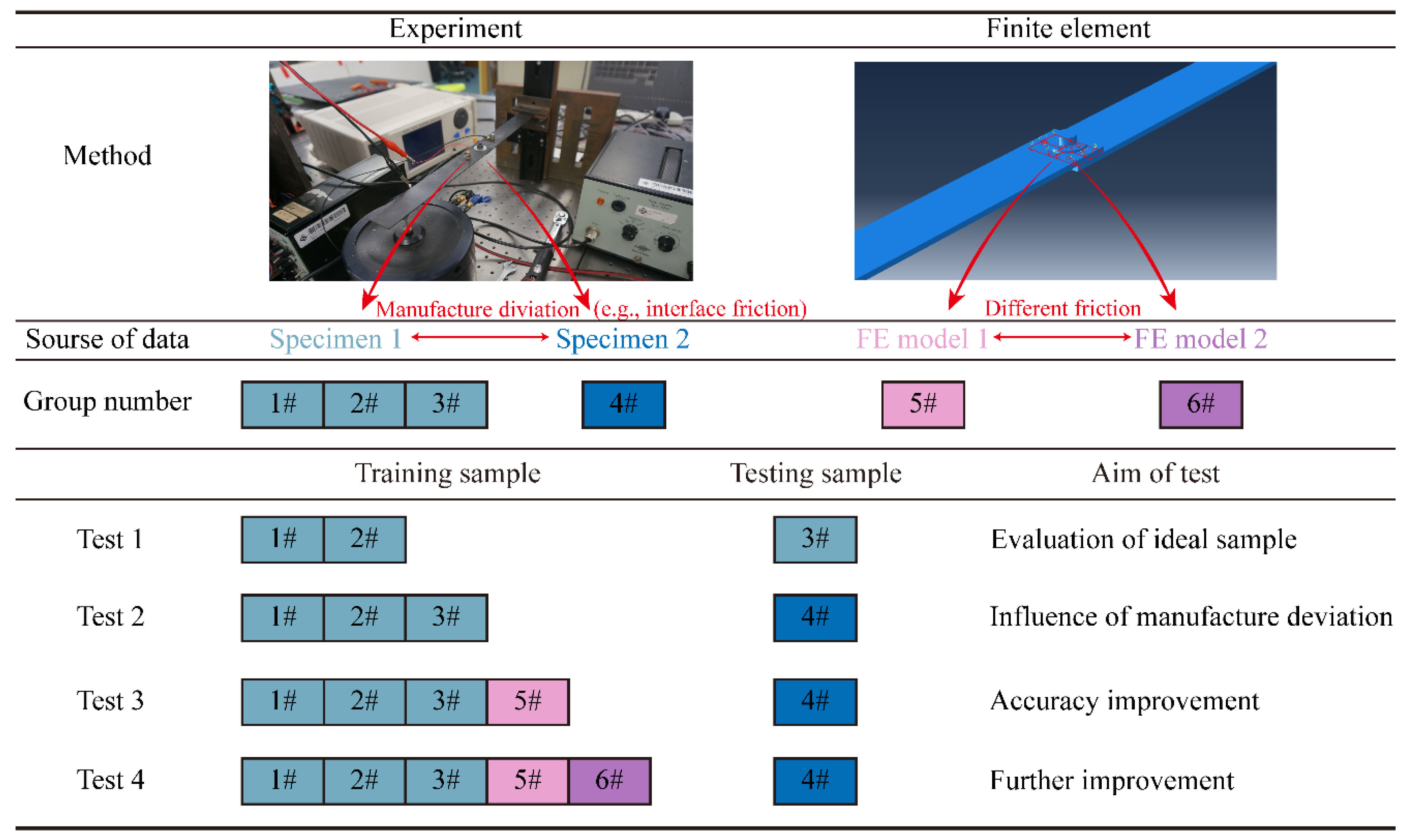
6.2. Arrangement for SVR Modeling and Prediction

The data set of each group was a 6 × 10 matrix, whose 10 columns corresponded to the preload levels (i.e., y_i∈{1, 2, 3, 4, 5, 6, 7, 9, 11, 13}) and the 6 rows consisted of the amplitudes of linear and nonlinear features (i.e., x_i = {A_LF, A_SOH, A_TOH, A_LS, A_HF, A_RS}^T). The data in each row (i.e., the amplitudes of each feature for different preloads) were normalized within a range of 0~1 before being input to the model.

Figure 9 shows the flow of the tests and the source of data. Data groups 1~3 and 4 were all collected from the experiment with joints of the same size and material parameters. The difference was that groups 1~3 were the repeated VAM results from specimen 1, while group 4 was collected from a new specimen, which may have possessed some slight manufacture deviations (e.g., interface friction or clamping boundary) compared to specimen 1. Groups 5 and 6 were collected from the same numerical model with different friction coefficients τ. The friction coefficients τ of group 5 were 0.1 for the Al–Al joints and 0.2 for the C–C joints, respectively. The coefficients of group 6 were 0 for the Al–Al joints and 0.4 for the C–C joints.

A total of eight tests were conducted using the SVR method for the Al–Al joints (four tests) and C–C joints (four tests), the test flows for the two materials were the same. In test 1, groups 1 and 2 were input to the SVR model as training samples, and group 3 was used to validate the predicted results. The evaluation of test 1 was carried out under ideal conditions without deviation between the specimens. In test 2, the SVR model was trained by groups 1~3 and validated by group 4 in order to reveal the variation int he evaluation accuracy due to manufacturing deviations between the different specimens. In tests 3 and 4, FEM samples 5 and 6 were adding to the training data to improve the applicability and accuracy of the SVR prediction by simulating the deviation of the frictional conditions.

The parameter v for the v-SVR model was 0.5 and the optimization based on grid search (GS) was used to choose the penalty parameter c and the kernel parameter σ. The parameters are shown in

Table 2. SVR parameters c and σ.

		Test 1	Test 2	Test 3	Test 4
Al–Al	c	11.3137	181	256	1.414
	σ	0.0884	0.0221	0.02	0.25
C–C	c	181	5.657	2.828	4
	σ	0.1768	0.125	0.5	0.354

.

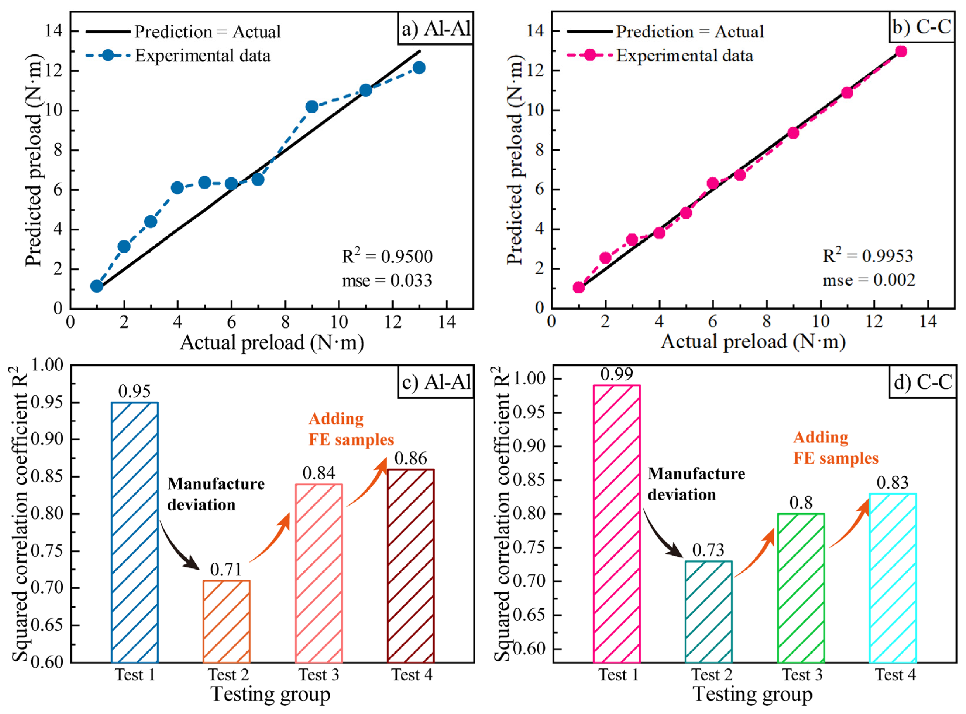
6.3. Results of Intelligent Prediction

The results of the preload prediction of SVR are shown in Figure 10. In test 1 (Figure 10a,b), the predictions on the experimental data using the SVR model trained by the samples from the same source were the most accurate (R² = 0.95 for the Al–Al joints and R² = 0.99 for the C–C joints). Compared to the C–C model, the Al–Al model saw bigger errors in the prediction at the beginning of the loading (2~5 N·m). This may be because the Al–Al interface was harder than the C–C one, so the early-stage deformation of the Al–Al interfaces of different specimens was not simultaneous. When the Al–Al joints were subjected to the high-tightening torque (6~14 N·m), the error decreased.

Generally, the SVR model, driven by the amplitudes of the nonlinear features collected from the VAM experiment, was an effective method for the evaluation of bolt loosening. Compared to the nonlinear coefficients, the SVR model efficiently identified the differences among the data sets in the high-stress states, and the prediction curve was more linear, which allowed for the efficient early-stage warning of bolt loosening and the long-term SHM under the combined influences of the nonlinearities.

Comparatively, in Figure 10c,d, the predictions of the preloads of specimen 2 trained by the samples from specimen 1 show the lowest accuracy (R² = 0.71 for the Al–Al joints and R² = 0.73 for the C–C joints). Based on the assumption that the decrease in accuracy from test 1 to test 2 was partially because of the deviation in the interface friction, the FE data for different friction coefficients τ were added to the machine training. The bar chart shows that the accuracy of the prediction rose gradually due to the aid from the FE data.

6.4. Discussion

Simulation data have rarely been applied to machine training before this study, which may be because the FEM has its limitations in simulating all of the actual experimental conditions. However, the increasing trends in Figure 10c,d show a possible improvement in machine training by expanding the sample abundance using the FEM to simulate the potential deviations.

The method that trains the AI model using data from a combination of simulation and experiments shows some advantages and limitations, as follows:

• The simulated data have good applicability for considering deviations in the experimental specimens. This method is cost-efficient by avoiding collecting many experimental samples, which are not accessible in certain circumstances (e.g., small-sample applications).
• However, the simulated results can change remarkably with changes in the FE parameters. This is due to the error accumulation during the iterative calculation of FE software. So, it would be better if FE modeling was based on adequate advanced knowledge of the potential influence factors (such as their types and values).
• Despite Point 2, the prediction robustness can still be guaranteed when inputting enough experimental results as training data, which enables the simulated samples to fully consider the different conditions.

7. Conclusions

The bolt preload evaluation for C–C and Al–Al joints was investigated using a VAM experiment and finite element simulation.

The combined influences of CAN, MIN, and DN on the signal amplitudes and nonlinear coefficients in the VAM test were investigated. As a result, measurable dissipation occurred on the HF amplitudes and was affected by the interface friction, leading to the deviation of the nonlinear coefficient when measuring the preload. In addition, the variation in the nonlinear coefficients at high-stress states became slight under the dominance of MIN, which made the early-stage warning of bolt loosening more difficult.

The SVR method, making full use of the amplitudes of the spectral linear and nonlinear responses, was developed to solve the inherent deficiency of the nonlinear coefficients when evaluating bolt loosening at the early stage. The SVR evaluation of bolt preloads showed better accuracy and applicability than conventional nonlinear coefficients for all stress stages. The SVR prediction, whose training and testing data were from different specimens, had lower accuracy than that from the same specimens due to manufacturing deviations. By adding the simulation data from the FE model with different friction coefficients and simulating the manufacturing deviations, the lowest prediction accuracy increased. The usage of FE data shows good potential to improve the AI prediction of bolt loosening in actual engineering structures.

References

1. Yun, H.; Rayhana, R.; Pant, S.; Genest, M.; Liu, Z. Nonlinear ultrasonic testing and data analytics for damage characterization: A review. Measurement 2021, 186, 110155. [Google Scholar] [CrossRef]
2. Du, F.; Wu, S.; Xing, S.; Xu, C.; Su, Z. Temperature compensation to guided wave-based monitoring of bolt loosening using an attention-based multi-task network. Struct. Health Monit. 2022. [Google Scholar] [CrossRef]
3. Chen, D.; Shen, Z.; Fu, R.; Yuan, B.; Huo, L. Coda wave interferometry-based very early stage bolt looseness monitoring using a single piezoceramic transducer. Smart Mater. Struct. 2022, 31, 035030. [Google Scholar] [CrossRef]
4. Zhang, Z.; Liu, M.; Liao, Y.; Su, Z.; Xiao, Y. Contact acoustic nonlinearity (CAN)-based continuous monitoring of bolt loosening: Hybrid use of high-order harmonics and spectral sidebands. Mech. Syst. Signal Process. 2018, 103, 280–294. [Google Scholar] [CrossRef]
5. Guan, R.; Lu, Y.; Wang, K.; Su, Z. Fatigue crack detection in pipes with multiple mode nonlinear guided waves. Struct. Health Monit. 2018, 18, 180–192. [Google Scholar] [CrossRef]
6. Kudela, P.; Radzienski, M.; Ostachowicz, W. Impact induced damage assessment by means of Lamb wave image processing. Mech. Syst. Signal Process. 2018, 102, 23–36. [Google Scholar] [CrossRef]
7. Solodov, I.Y.; Krohn, N.; Busse, G. CAN: An example of nonclassical acoustic nonlinearity in solids. Ultrasonics 2002, 40, 621–625. [Google Scholar] [CrossRef]
8. Yang, Y.; Ng, C.-T.; Kotousov, A. Bolted joint integrity monitoring with second harmonic generated by guided waves. Struct. Health Monit. 2018, 18, 193–204. [Google Scholar] [CrossRef]
9. Zhang, M.; Shen, Y.; Xiao, L.; Qu, W. Application of subharmonic resonance for the detection of bolted joint looseness. Nonlinear Dyn. 2017, 88, 1643–1653. [Google Scholar] [CrossRef]
10. Croxford, A.J.; Wilcox, P.D.; Drinkwater, B.W.; Nagy, P.B. The use of non-collinear mixing for nonlinear ultrasonic detection of plasticity and fatigue. J. Acoust. Soc. Am. 2009, 126, 117–122. [Google Scholar] [CrossRef]
11. Jiao, J.; Meng, X.; He, C.; Wu, B. Nonlinear Lamb wave-mixing technique for micro-crack detection in plates. NDT E Int. 2017, 85, 63–71. [Google Scholar]
12. Huan, Q.; Chen, M.; Su, Z.; Li, F. A high-resolution structural health monitoring system based on SH wave piezoelectric transducers phased array. Ultrasonics 2019, 97, 29–37. [Google Scholar] [CrossRef] [PubMed]
13. Zhang, Z.; Xu, H.; Liao, Y.; Su, Z.; Xiao, Y. Vibro-acoustic modulation (VAM)-inspired structural integrity monitoring and its applications to bolted composite joints. Compos. Struct. 2017, 176, 505–515. [Google Scholar] [CrossRef]
14. Wang, F.; Song, G. Bolt early looseness monitoring using modified vibro-acoustic modulation by time-reversal. Mech. Syst. Signal Process. 2019, 130, 349–360. [Google Scholar] [CrossRef]
15. Wang, F.; Song, G. Monitoring of multi-bolt connection looseness using a novel vibro-acoustic method. Nonlinear Dyn. 2020, 100, 243–254. [Google Scholar] [CrossRef]
16. Qin, X.; Peng, C.; Zhao, G.; Ju, Z.; Lv, S.; Jiang, M.; Sui, Q.; Jia, L. Full life-cycle monitoring and earlier warning for bolt joint loosening using modified vibro-acoustic modulation. Mech. Syst. Signal Process. 2022, 162, 108054. [Google Scholar] [CrossRef]
17. Zaitsev, V.Y.; Matveev, L.A.; Matveyev, A.L. Elastic-wave modulation approach to crack detection: Comparison of conventional modulation and higher-order interactions. NDT E Int. 2011, 44, 21–31. [Google Scholar] [CrossRef]
18. Klepka, A.; Staszewski, W.; Jenal, R.; Szwedo, M.; Iwaniec, J.; Uhl, T. Nonlinear acoustics for fatigue crack detection—Experimental investigations of vibro-acoustic wave modulations. Struct. Health Monit. 2012, 11, 197–211. [Google Scholar] [CrossRef]
19. Li, N.; Sun, J.; Jiao, J.; Wu, B.; He, C. Quantitative evaluation of micro-cracks using nonlinear ultrasonic modulation method. NDT E Int. 2016, 79, 63–72. [Google Scholar] [CrossRef]
20. Broda, D.; Staszewski, W.J.; Martowicz, A.; Uhl, T.; Silberschmidt, V.V. Modelling of nonlinear crack–wave interactions for damage detection based on ultrasound—A review. J. Sound Vib. 2014, 333, 1097–1118. [Google Scholar] [CrossRef]
21. Biwa, S.; Nakajima, S.; Ohno, N. On the Acoustic Nonlinearity of Solid-Solid Contact With Pressure-Dependent Interface Stiffness. J. Appl. Mech. 2004, 71, 508–515. [Google Scholar] [CrossRef]
22. Zhang, Z.; Liu, M.; Su, Z.; Xiao, Y. Quantitative evaluation of residual torque of a loose bolt based on wave energy dissipation and vibro-acoustic modulation: A comparative study. J. Sound Vib. 2016, 383, 156–170. [Google Scholar] [CrossRef]
23. Fillinger, L.; Zaitsev, V.Y.; Gusev, V.; Castagnede, B. Nonlinear relaxational absorption/transparency for acoustic waves due to thermoelastic effect. Acta Acust. United Acust. 2006, 92, 24–34. [Google Scholar]
24. Nazarov, V.E.; Radostin, A.V.; Soustova, I.A. Effect of an intense sound wave on the acoustic properties of a sandstone bar resonator. Experiment. Acoust. Phys. 2002, 48, 76–80. [Google Scholar] [CrossRef]
25. Parsons, Z.; Staszewski, W.J. Nonlinear acoustics with low-profile piezoceramic excitation for crack detection in metallic structures. Smart Mater. Struct. 2006, 15, 1110. [Google Scholar] [CrossRef]
26. Zimenkov, S.V.; Nazarov, V.E. The dependence of damping of ultrasound by sound in annealed copper on the frequency of the sound. Sov. Phys.-Acoust. 1992, 38, 4. [Google Scholar]
27. Meo, M.; Polimeno, U.; Zumpano, G. Detecting Damage in Composite Material Using Nonlinear Elastic Wave Spectroscopy Methods. Appl. Compos. Mater. 2008, 15, 115–126. [Google Scholar] [CrossRef]
28. Zaitsev, V.; Gusev, V.; Castagnede, B. Luxemburg-gorky effect retooled for elastic waves: A mechanism and experimental evidence. Phys. Rev. Lett. 2002, 89, 105502. [Google Scholar] [CrossRef] [Green Version]
29. Solodov, I.; Wackerl, J.; Pfleiderer, K.; Busse, G. Nonlinear self-modulation and subharmonic acoustic spectroscopyfor damage detection and location. Appl. Phys. Lett. 2004, 84, 5386–5388. [Google Scholar] [CrossRef]
30. He, Y.; Xiao, Y.; Su, Z.; Pan, Y.; Zhang, Z. Contact acoustic nonlinearity effect on the vibro-acoustic modulation of delaminated composite structures. Mech. Syst. Signal Process. 2022, 163, 108161. [Google Scholar] [CrossRef]
31. Zhou, Y.; Xiao, Y.; He, Y.; Zhang, Z. A detailed finite element analysis of composite bolted joint dynamics with multiscale modeling of contacts between rough surfaces. Compos. Struct. 2020, 236, 111874. [Google Scholar] [CrossRef]
32. Dao, P.B.; Klepka, A.; Pieczonka, Ł.; Aymerich, F.; Staszewski, W.J. Impact damage detection in smart composites using nonlinear acoustics—Cointegration analysis for removal of undesired load effect. Smart Mater. Struct. 2017, 26, 035012. [Google Scholar] [CrossRef]
Figure 1. Simplified model of a joint subjected to two harmonic forces.
Applsci 12 12920 g001
Figure 2. Finite element model of the bolted joints: (a) assembling, (b) geometric parameters, (c) load and boundary conditions, (d) mesh.
Applsci 12 12920 g002
Figure 3. Experimental system.
Applsci 12 12920 g003
Figure 4. Acceleration contour of VAM progress.
Applsci 12 12920 g004
Figure 5. Acceleration contours of interface under different preloads: (a) 1 N·m, (b) 3 N·m, (c) 9 N·m, (d) 13 N·m.
Applsci 12 12920 g005
Figure 6. Waveforms of the Al–Al bolted joint in time domain: (a) experiment, (b) FEM.
Applsci 12 12920 g006
Figure 7. Typical frequency spectra of the Al–Al bolted joint: (a) experiment, (b) FEM.
Applsci 12 12920 g007
Figure 8. Simulated and experimental nonlinear coefficients and their influence factors.
Applsci 12 12920 g008
Figure 9. Flow of SVR modeling and evaluation.
Applsci 12 12920 g009
Figure 10. SVR prediction results. (a) results of test 1 for Al-Al joints, (b) results of test 1 for C-C joints, (c) variation of correlation coefficient from test 1 to test 4 for Al-Al joints, (d) variation of correlation coefficient from test 1 to test 4 for C-C joints.
Applsci 12 12920 g010