A Combined Machine Learning and Model Updating Method for Autonomous Monitoring of Bolted Connections in Steel Frame Structures Using Vibration Data

Abstract

This research paper presents a novel structural health monitoring strategy based on a hybrid machine learning and finite element model updating method for the health monitoring of bolted connections in steel planer frame structures using vibration data. Towards this, a support vector machine model is trained with the discriminative features obtained from time history data, and those features are used to distinguish between damaged and undamaged joints. An FE model of the planer frame is considered where the fixity factor (FF) of a joint is modeled with rational springs and the FF of the spring is assumed as the severity level of loosening bolts. The Cat Swarm Optimization technique is further applied to update the FE model to calculate the fixity factors of damaged joints. Initially, the method is applied to a laboratory-based experimental model of a single-story planer frame structure and later extended to a pseudo-numerical four-story planer frame structure. The results show that the method successfully localizes the damaged joints and estimates their fixity factors.

1. Introduction

Due to the aesthetic ability of human beings and the exigencies of economic development, magnificent infrastructures such as bridges, skyscrapers, tunnels, and dams have been constructed for centuries. However, structures inevitably degrade over time. Among these structures, those constructed using steel are more susceptible to damage at connections between members due to corrosion, cyclic loads, and unexpected loads for which the structures are not designed. Following connection damage, the performance of the structure degrades [1]. To avoid sudden failure and to provide the reliability of the structure, structural health monitoring (SHM) strategies are employed to periodically monitor the performance of the structure. For the SHM of joints, various local approaches, namely, acoustic emission (AE) [2], image classification [3,4], and impedance-based techniques [5], are being applied in practice. However, these local techniques are impractical for civil engineering structures as a large number of sensors are required and even placing such sensors is difficult at joints. Therefore, vibration-based global health monitoring techniques, namely, model-based and signal-based, are found to be applied for the health monitoring of civil engineering structures [6,7,8,9,10]. The ability to quantify damage-sensitive parameters made the model-updating technique popular with scientists and engineers. Various approaches to the finite element model updating technique and their applications to different types of structures can be found [11,12,13,14,15]. The two-phase health monitoring of a beam and a plate type of structure were found to be carried out using a genetic algorithm and the Eigen-sensitivity method [11]. A hybrid real genetic algorithm was applied for the health monitoring of a space frame structure to the set-up of the GA parameters and operators. Various objective functions were examined for accuracy [12]. A multi-stage and multi-objective optimization was also found to be applied in the field of SHM of civil engineering structures [13,14]. A vision-based FE model updating technique was also applied to the SHM of a three-storey building frame structure, which was found to reduce cost and time [15]. However, the success of the technique depends on multiple factors, namely, the accuracy of the finite element (FE) model, the quality of experimental data, the optimization algorithm, and the definition of the optimization algorithm. In FE-based model updating, FE models of the physical systems are developed and updated to achieve a good agreement with experimental data. In the process, a detailed FE model with a large number of elements and several updating parameters is required to recognize the effect of localized damage. However, these may increase the computational cost as well as may make the solution ill-conditioned. Teughels et al. [16] presented a parameterization method, namely, a damage function for reducing the number of updating variables. The technique assumes correction factors for updating parameters that change continuously over the FE modeling. The technique was applied to an RCC beam [16]. A multi-stage damage detection technique was proposed by Perera and Ruiz [17] for the monitoring of a large-scale structure. In the primary stage, expected damage points were approximated and in the next stage, the exact location of the damage and severity was estimated. Pal and Banerjee [18] also proposed modal strain energy in combination with FE model updating for the health monitoring of joints of a planer frame structure to identify accurate damage location and quantity. Wu and Li [19] proposed a two-step FE model updating. The technique was applied to the ASC benchmark building, where, in the first stage, connection stiffness and young’s modulus were identified and then applying the FE model updating, the estimation of damaged braces was carried out [19]. Wen and Songye [20] developed a progressive damage identification strategy depending on a multiple-scale wavelet FE model that was successfully examined on a numerical model of a beam and a frame. An enhanced substructure-oriented response sensitivity method was proposed for the health monitoring of a large-scale structure for accurate estimation of damage [21]. However, directly or indirectly, all the above-mentioned techniques focus on the reduction of the number of variables or accurate estimation of the damage-sensitive parameters.

Machine learning (ML) algorithms have also recently been found to be applied in the field of SHM and damage detection. The model updating technique considers a reference model and updates to represent a damaged structure to determine the damage-sensitive parameters. However, ML is a data/image-based technique which builds a model for mapping input patterns to output targets [22]. Sikdar and Pal [23] utilized the Bag of Visual Words based scalogram image classification approach to classify dis-bonds at different locations of a composite plate structure. To generate a large number of datasets, they carried out multiple experimental trials for each of the healthy and damaged cases. In order to test the learning algorithm, data were collected from a smaller size disbond level. However, their study was not able to give an idea about the disbond sizes. Liu and Zhang [24] utilized the convolutional neural network (CNN) technique for the inspection of post-hazard ultra-low cycle fatigue-related damage in structural steel fuse members. They defined a micromechanical damage index for various levels of damage to quantitatively cluster the data. In their study, they considered five classes of damage levels. In Kundu et al. [25], an Acoustic Emission (AE) signal-based ML algorithm was trained for the monitoring of a carbon fiber composite panel using various statistical features and the k nearest neighbor (KNN) algorithm. A Naïve Bayes data fusion scheme and CNN-based framework were proposed by Chen and Jahanshahi [26] for the crack detection of a metallic structure. Time-varying damage index-based features were fed into a CNN algorithm to localize the damages in a plate type of structure by Zhang et al. [27]. A few more applications of the ML technique in SHM are presented in [28,29,30,31,32,33]. Again, inside Tsinghua University, post-seismic event-based damage assessment for 619 buildings was carried out based on CNN using the time-frequency domain representation of acceleration ground motion [34]. A combination of a probabilistic neural network and finite element model updating was found to assess the condition of a truss bridge structure [35]. Image-based deep learning and graphical model is used for the detection of the loosening of bolts [36]. Auto-Regressive Integrated Moving-Average Machine Learning for Damage Identification of Steel Frames has also been found to be available in the domain of SHM under different EQ excitation. Damages were created by the loosening of bolts of the bracing members [37]. The application of ML is found to be increasing in recent times as automation of SHM is a felt need. However, studies show that for accurate prediction of damage severity and location, a large number of damage classes and corresponding training data sets are required that are somewhat impractical for civil engineering structures.

In this paper, a novel vibration data-based hybrid ML and FE model updating method for the accurate estimation of joint damage and its severity is presented. The method is initially applied on an experimental small-scale single-story bolted joint planer frame model, and further extended to a four-story pseudo numerical model of a steel planer frame structure. The study is carried out to address the following objectives:

(i)

The development of a combined ML and FE model updating technique for the health monitoring of joints of planer frame structures;

(ii)

The accurate localization and quantification of joint damage with a lesser number of data sets compared to the data sets required if only either the ML-based technique or model updating technique is employed for the same purpose;

(iii)

The effectiveness of standard deviation, skewness, kurtosis, mean absolute deviation, and entropy-based features for the localization of loosening of bolts in planer frame structures.

2. Methodology

This paper presents a novel vibration data-based hybrid ML and model updating method to identify the damage location and quantity of the loosening of bolts in a steel frame structure. Figure 1 describes the working procedure of the method. It has been found that machine learning techniques require a large number of data sets for each of the damaged and undamaged cases. For a civil engineering structure, obtaining so much data is quite a difficult task. Moreover, the model updating techniques produce inaccurate results in the presence of a large number of variables. Hence the problem was divided into two parts—(1) localization and (2) quantification. The machine learning algorithm was used to approximately localize the loosening of bolts. Considering the fixity factors at the approximate locations as variables, the model updating operation was carried out to identify the exact location of the loosening of the bolts and quantity. By employing the machine learning algorithm, the number of variables can be drastically reduced.

2.1. Machine Learning Based Localization

In order to detect the approximate position of the loosening of bolts, the strain data were categorized as healthy (H) and loosened (L) cases. The H case consists of strain data collected from the sensors placed at the location where loosening is not there (i.e., the sensors are placed far away from the joints). The (L) case represents the strain data corresponding to the sensors placed near the location of the loosening of bolts. The main idea of this categorization is that the sensors near the location of the loosening of bolts will show different features than the other sensors. In this paper, three entropy-based features, namely, approximate entropy, Shannon entropy and Renyi’s entropy along with three statistical features, namely, variance, kurtosis and skewness were considered. The detail of these features is given below.

2.1.1. Feature Extraction

As the data were categorized into H or L cases, first, the strain data of all sensors were normalized concerning the highest strain value of data over all the trials. With this normalization, it could be assumed that the data are stored from an equal energy level. Therefore, the parameters of the data will be affected because of the loosening of bolts only.

Approximate entropy (ApproximateEnt): The ApproximateEnt is a function that generates a delayed-reconstruction: y_1:n corresponding to ‘n’ data points and embedding dimension ‘d’. The number at a point ‘i’ within the selected range is calculated [38]:

$$n_i={\displaystyle \sum _{i=1,i\ne j}^{n}1\left({‖y_i-y_j‖}_{\infty }<r\right)}$$

(1)

where ‘r’ depicts the radius of similarity. The approximate entropy is computed as

$$ApproximateEnt={\phi }_d-{\phi }_{d+1}$$

(2)

where,

$${\phi }_d={(n-d+1)}^{-1}{\displaystyle \sum _{i=1}^{n-d+1}\log \left(n_i\right)}$$

(3)

Shannon entropy (ShanonE_n): In ShanonEn calculation, the power of every frequency (j_f) is multiplied by the logarithm of the inverse power of each frequency and calculated by summing across all frequencies (J_f) as described in Equation (5) [39].

$$j_f=\frac{J_f}{{\displaystyle \sum J_f}}$$

(4)

$$Shanon{E}_n={\displaystyle \sum _f{j}_f\log \left(\frac{1}{j_f}\right)}$$

(5)

Reniy entropy (RenyE_n): Renyi’s entropy is used for the estimation of the spectral complexity of time-series which is defined as [39]:

$$RenyiEn\left(\beta \right)=\frac{1}{\left(1-\beta \right)}\log \left({\displaystyle \sum _f{P}_f^{\beta }}\right),\beta >0,\beta \ne 1$$

(6)

In this study, $\beta =2$ is considered to compute Renyi’s quadratic entropy which represents the uncertainty level about the event, ‘f’.

Mean Absolute deviation (MAD): It is used to address the statistics of various fundamental processes. Here, MAD is defined as [40]:

$$MAD=\frac{1}{m}{\displaystyle \sum _{m=0}^{m-1}\left|{\mu }_i\left[M\right]-{\kappa }_i\right|}$$

(7)

where ‘${\kappa }_i$’ represents the mean of the ith Fourier-intrinsic-band-function, ‘${\mu }_i\left[M\right]$’ and $0\le M\le m-1$.

Four other statistical features, namely, standard deviation, variance, skewness, and kurtosis are also considered in this paper as described in [41,42,43].

The feature sets for all the unloosed and loosened cases were kept separately and provided as input for the SVM algorithm to train and validate the SVM model. After, the trained and validated model was employed to test the data sets. In this context, the test data sets were given as input for the SVM model.

2.1.2. Classification Using SVM

SVM is a machine learning technique used as a supervised classification technique that produces a model using training data sets and maps new data sets [37]. It can be better understood by a two-class problem. The main aim of SVM is to find an optimal margin (hyper-plane) from a set of planes that separates the data point of the two classes. The plane which has the maximum margin is called a hyper-plane. A large margin decision boundary tends to generate better generalization error and a smaller margin corresponding to a small perturbation to the decision boundary can have a significant impact on the classification performance and may lead to an overfitting problem. More detail about SVM can be found in [37].

SVM is used to classify the feature set calculated from the data obtained from healthy and various loosening cases. SVM parameters are picked out by training the model. The performance of SVM is contingent upon the kernel selection, appropriate kernel parameters, and soft margin parameter ‘P’. In the study, a Gaussian kernel with a single parameter, ‘$\eta$’ is selected and an optimum combination of ‘P’ and ‘$\eta$’ can be selected based on a grid-search based on the exponentially growing sequences, such as in the given example:

$$\begin{array}{l}P\in \left[2^{-7},2^{-5},{\dots 2}^{11},2^{13}\right]\\ \eta \in \left[2^{-7},2^{-5},{\dots 2}^3,2^5\right]\end{array}$$

(8)

In the process, using cross-validation, the choice of each combination of the parameter is examined. The parameters having the highest accuracy in cross-validation are culled. The selected SVM model for testing and classification of a new dataset is further trained using the entire training dataset based on the chosen parameters [23].

Three-different polynomial kernels with orders 1, 2, and 3 are tested. A tenfold validation was carried out to check the classifier’s performance. The classification performance of the trained SVM model is obtained for the test datasets and the unicity of this model is its decision boundary is dependent on a subset of the training dataset (i.e., support vectors) as presented in [23]. For the given training set ‘X’ and corresponding labels ‘Y’ (i.e., ±1), the classification function for the 2-class problem described above can be defined as [23]:

$$f(X)=sign(w^{T}X+w_0)$$

(9)

where ‘w’ and ‘w₀’ are the parameters of the hyperplane.

If the data are not linearly separable, an error weighting constant is considered as the penalty for misclassification and the original data space is mapped to feature space. In the kernel (C) formulation, the decision function can be given as follows:

$$f(\chi )=sign\left[{\displaystyle \sum _i{Y}_i{\zeta }_{i}C(\chi ,{\chi }_i)+w_0}\right]$$

(10)

where ‘${\chi }_i$’ is the training features obtained from data ‘$\chi$’ and the corresponding label is $Y_i$. ${\zeta }_i$ is ‘0′ for most ‘i’. The feature vectors are nothing but the support vector. For multi-class classification, this binary SVM model using the one-versus-one approach is considered. For the ‘N’ class problem, the number of learners is given by

$$F=N(N-1)/2$$

(11)

2.2. FE Model Updating Using CSO

In the case of the model updating, an FE model as presented in Figure 2a is developed and updated to determine the optimum value of the damage-sensitive parameters. With that purpose, 2 node frame elements are utilized to model the steel planer frame. In the element, each node is considered to have 3 degrees of freedom (two translational and one rotational). The generation of elemental stiffness and mass matrices are presented below.

2.2.1. Formulation of the Elemental Mass and Stiffness Matrices

Semi-rigid boundary conditions are assumed to define the loosening of bolts at joints. At the boundary, the semi-rigidity is ensured by considering rotational springs for each of the elements. Figure 2b represents the deformed shape of the element. In between the internal and outer sides of the spring, a relative rotation is considered. On the internal side of the spring, the rotations are $L{\theta }_1$, $R{\theta }_1$ while on the outer face, these rotations are $L{\theta }_2$, $R{\theta }_2$, respectively. Monforton and Wu (1963) [44] provide a relationship among the moment applied, rotational spring stiffness and internal and outer rotations:

$$\frac{RM}{R{r}_c}=R{\theta }_2-R{\theta }_1\mathrm{and}\frac{LM}{L{r}_c}=L{\theta }_2-L{\theta }_1$$

(12)

In Equation (12) given above, LM, $RM$, $L{r}_c$ and $R{r}_c$ are the moments applied at the spring and stiffness of rotational spring at the right and left end of each element. Element level stiffness-matrix and mass-matrix are then generated assuming the semi-rigid support conditions [45,46]. In [44], the relationship between the fixity factors of rotational springs with stiffness is defined by

$${\alpha }_{L{r}_c}=\frac{1}{1+\frac{3EI/L}{L_{r_c}}}\mathrm{and}{\alpha }_{R{r}_c}=\frac{1}{1+\frac{3EI/L}{R_{r_c}}}$$

(13)

In Equation (13), L, E and I represent element-length, elastic modulus, and the moment of inertia, respectively. For a different types of connections, Eurocode 3, as given in the following

Table 1. Designation of connections concerning FF as per Eurocode-3.

Quantity	Pin Joint	Semi-Rigid Joint	Rigid Joint	Quantity
FF	0–0.143	0.143–0.891	0.891–1	FF

, specifies the ranges of the fixity factor.

After the numerical modeling, the model updating operation is performed by applying CSO to quantify the level of FFs at the joints. The model updating procedure for the study is presented in the following paragraph.

2.2.2. Objective Function Formulation and Parameter Selection

The procedure starts with the formulation of an objective function and the selection of parameters. The effectiveness of any optimization technique greatly depends on the formulation of this function. In this paper, the damage-sensitive quantities, namely, natural frequencies, the maximum amplitude of frequencies and shape correlation between experimental and numerical models of a planer frame structure are considered to formulate the objective function.

The Newmark-Beta method was used for the calculation of dynamic responses. The displacement time-histories are calculated to generate strain time responses based on the strain-displacement relationship:

$${\epsilon }_n\left(t\right)=-y{x}_n(t{)}^{″}$$

(14)

where the extreme fiber distance of a section calculated from the neutral axis is y and a double dash over x(t) indicates the double derivative of the displacement at that section. Suffix n represents the numerical FE model. Further, the strain time history is transferred to the frequency domain using the following expression:

$${\epsilon }_n\left(\omega \right)=\frac{1}{2\pi }{\displaystyle {\int }_{-\infty }^{\infty }{\epsilon }_n}\left(t\right)e^{-iet}dt$$

(15)

where ω stands for frequency and ${\epsilon }_n\left(\omega \right)$ indicates amplitude corresponding to the frequency. For the experimental study, the strain dataset can be directly registered and transformed to the frequency domain using Fourier transform:

$${\epsilon }_{\exp }\left(\omega \right)=\frac{1}{2\pi }{\displaystyle \underset{-\infty }{\overset{\infty }{\int }}{\epsilon }_{\exp }\left(t\right)}{e}^{-i\omega t}dt$$

(16)

In Equation (16) given above, exp stands for the experimental case. For ith strain sensor, the frequency shape co-relation utilizing experimental and numerical strain data are obtained as:

$${\psi }_i=\frac{{\displaystyle \sum {\epsilon }_{n,i}\left(\omega \right){\epsilon }_{\exp ,i}\left(\omega \right)}}{{\left[{\epsilon }_{n,i}^2\left(\omega \right)\right]}^{1/2}{\left[{\epsilon }_{\exp ,i}^2\left(\omega \right)\right]}^{1/2}}$$

(17)

Equation (17) clearly states that if numerical and experimental structures are in the same condition then the shape co-relation value is about 1 and if they are not in the same condition and the value is deviating from 1. Finally, the objective function is formulated as:

$$OF({\alpha }_{L{r}_c},{\alpha }_{R{r}_c})={{\displaystyle \sum _{j=1}^{NT}\left[{{\displaystyle {\sum }_{i=1}^{NS}{\mathrm{W}}_i[{\{\epsilon {(\omega )}_{num}-\epsilon {(\omega )}_{\exp }\}}^2+{\{\omega {(\mathrm{A}\mathrm{M}{\mathrm{P}}_{\max })}_{num}-\omega {(\mathrm{A}\mathrm{M}{\mathrm{P}}_{\max })}_{\exp }\}}^2]}}_i\right]}}_j$$

(18)

In the objective function (OF) presented by Equation (18), ‘num’ is numerical, ‘exp’ is experimental, ‘NT’ is number of trials, ‘NS’ is number of sensors, α_Lrc and α_Rrc represent the fixity factors for the left and right of each member. ω(AMP_max) indicates the natural frequency identified from the maximum amplitude of the frequency domain representation of the strain signal. A weight factor for each sensor, ‘W_i’ is defined as:

$$W_i=\frac{{\psi }_i}{{\displaystyle \sum {\psi }_i^2}}$$

(19)

2.2.3. Cat Swarm Optimization (CSO)

CSO is an optimization technique, proposed by Chu and Tsai (2007) [47], depending on the behavior of a cat. It is a population-based search technique and starts with the generation of the random position of the population over the D dimensional (numbers of parameters) space. In CSO, each of these populations is termed as cat. Each of the cats represents a probable solution inside the domain of search space. Along with the initial position of variables, it also generates initial velocity. The number of populations is decided based on the convergence test of the solution. For each cat, the objective function value is computed and the cat that has the best fitness value is stored. It would be better to mention here that the best cat means the values of the parameters that generate the minimum value of the objective function. The algorithm performs both local and global search in the name of seeking mode and tracing mode, respectively. Based on a mixture ratio, the cats are transferred to seeking and tracing mode. The positions of the cats in the seeking mode are updated based on the minimum function value of the copies of each cat. The detailed working procedure of CSO can be found in [44].

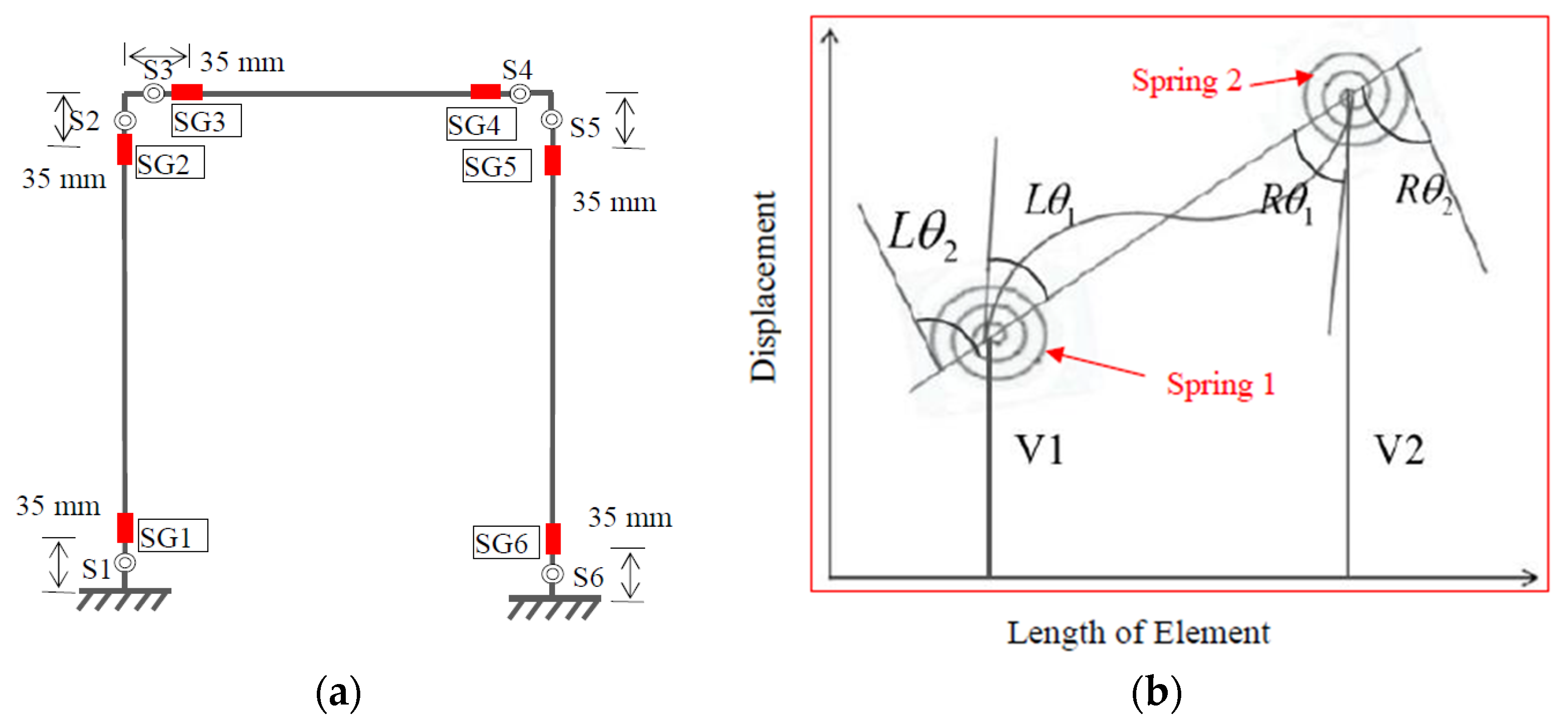
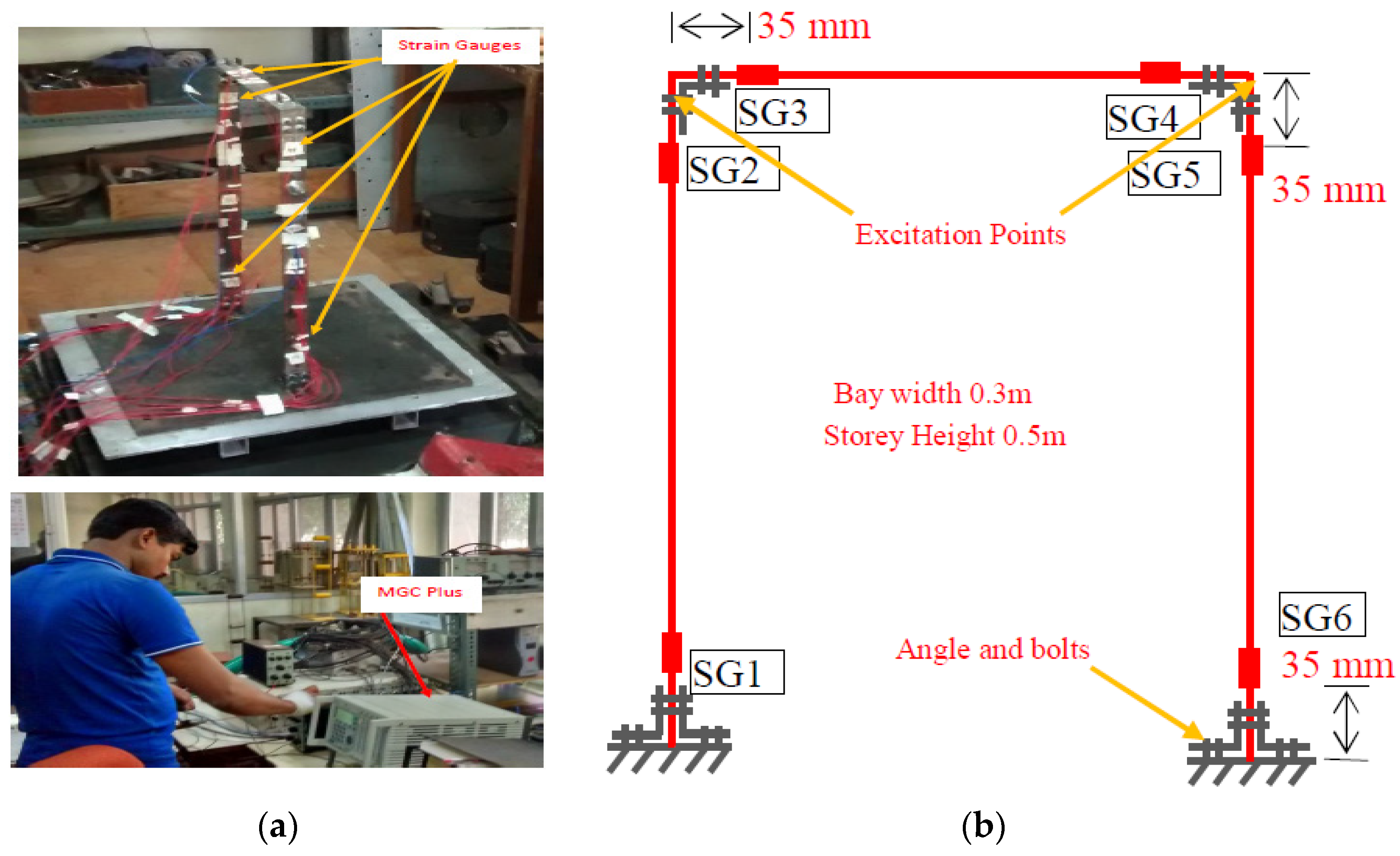
3. Experimental Study

In order to verify the effectiveness of the hybrid ML and MU technique, first, an experimental model of a bolted joint single-story steel planer frame structure as shown in Figure 3 is considered. The detailed fabrication and experimental procedure are explained in the experimental modeling section given below.

A single-storey planer frame structure as depicted in Figure 3 is utilized to estimate the level of severity of joint damage using the experimental data. The small-scale steel frame model was developed in the laboratory and the whole experimental study was conducted in the control environment of the Experimental Mechanics Laboratory of the Civil Engineering Department at IIT Bombay. The properties of the steel frame are Young’s modulus = 2.1 GPa, Poisson’s ratio = 0.3, and mass density = 7850 kg/m³. The width and depth of the members are 0.032 m and 0.006 m, respectively. The height of the column and the length of the beam are 0.5 m and 0.3 m, respectively. In this context, the members of the above-mentioned sizes and dimensions were available in the laboratory and utilized for the fabrication of the frame. In order to make the beam-column connections, angle sections and nut-bolts were used. At the side of the column face as well as at the side of the beam face of a joint, one angle and four M-5 nut-bolts are used for the proper beam-column connection. In order to generate fixed support for the frame, two angles are placed at the inner and outer faces of the column and tightly connected at the base using nut-bolts. The experimental study was carried out for unloosed conditions, i.e., all bolts are in full-tight condition (UL) and also for different loosening conditions at different connections (BL1 to BL6). The unloosened and different loosened conditions are further explained in detail in

Table 2. Experimental study case details.

Condition of Structure	Details of Loosening
UL	Bolts are fully tight
BL1	Right column-beam connection, bolts @ column face is hand tight
BL2	Right column-beam connection, bolts @ column face is full loose
BL3	Left column-beam connection, bolts @ beam face is hand tight
BL4	Right column-beam connection, bolts @ beam face is full loose
BL5	Left column-beam connection, bolts @ column face is hand tight
BL6	Left column-beam connection, bolts @ column face is full loose
BL7	Left column-beam connection, 2 bolts @ column face is full loose

and Figure 4. It is better to be mentioned here that unloosened condition means all bolts are fully-tight represents bolts are tightened using hand plus turned the bolts half using a spanner and the hand-tight represents that the bolts are tightened using hands.

A B & K made B & K 8202-8200, 31.6 mv/N impact hammer was employed to provide an impact at the top corner of the right beam-column connection as described in Figure 2b. The strain time responses were registered using 12-contact type strain sensors (FLA-3), from SG1 to SG6. Here, the contact type strain gauges were fixed on either side of the column/beam members at 35mm from the beam-column joints as shown in Figure 3. At SG1, 1-strain gauge is placed on the outer-face of the member and another strain gauge is placed inner-face of the member. Strain gauges are fitted in SG2 to SG6 position similarly. HBM-made MGC-plus data logger was utilized to collect the strain time history data with 600 Hz sampling frequency.

In order to approximately localize joint damage using the ML approach, strain time history data were categorized into “healthy” and “loosened” cases. In the experimental case of UL, all 12 strain gauges were provided with healthy data, thus, producing 120 healthy data sets in 10 trials. In cases BL1 and BL2, only the four strain gauges near the right joint are considered to be loosened data and the rest eight strain gauge data are considered healthy data. Therefore, each of BL1 and BL2 will produce 40 loosened data and 80 healthy data in 10 trials. Compared to the healthy data set, there were fewer loosened data; therefore, 10 more trials were carried out for BL1 and BL2 and only the loosened data were considered. Finally, a data pool was constructed with 280 healthy and 160 loosened data. The entire data distribution for the classification is given in

Table 3. Arrangement of the experimental data for training, validation, and testing.

Condition of Structures	Healthy Data	Loosened Data	Usage of Data	Remarks
UL	10 (trial) × 12 (sensors) = 120	-	Training + Validation	Training (100 healthy + 100 loosened) Validation (180 healthy + 60 loosened)
BL1	10 (trial) × 8 (sensors) = 80	20 (trial) × 4 (sensors) = 80
BL2	10 (trial) × 8 (sensors) = 80	20 (trial) × 4 (sensors) = 80
BL3	10 (trial) × 8 (sensors) = 80	10 (trial) × 4 (sensors) = 40	Testing	Testing (320 healthy + 160 loosened)
BL4	10 (trial) × 8 (sensors) = 80	10 (trial) × 4 (sensors) = 40
BL5	10 (trial) × 8 (sensors) = 80	10 (trial) × 4 (sensors) = 40
BL6	10 (trial) × 8 (sensors) = 80	10 (trial) × 4 (sensors) = 40
BL7	10 (trial) × 8 (sensors) = 80	10 (trial) × 4 (sensors) = 40	Testing

. It is assumed that sensor data reasonably close to the loosening of bolts will have some different features compared to the sensor data away from the loosened bolted joint because of the local chattering of bolts, washers, and members.

A sample strain time history collected at the location of SG2 is depicted in Figure 5a indicating that a significant portion of the data are not useful for this study. Hence, the informative data recorded after the impact was used for this research work and depicted in Figure 5b. A typical example of time history data obtained at SG2 for the UL case and its effective portion is shown in Figure 5a,b.

The normalized time history data were then utilized to determine the features as discussed in Section 2. After the collection of all feature sets from all the data, SVM was trained with the feature set distribution as given in Table 3. Finally, the remaining feature set was utilized for validation. A 10-fold cross-validation experiment was carried out to check whether the algorithm was really trained or just memorizing information. The confusion matrix shown in

Table 4. Confusion charts show the average training and validation accuracy for experimental models.

Case		Training		Case		Validation
		Healthy	Loosened			Healthy	Loosened
UL	Healthy	40	0	UL	Healthy	80	0
	Loosened	0	0		Loosened	0	0
BL1	Healthy	30	0	BL1	Healthy	40	10
	Loosened	15	35		Loosened	11	19
BL2	Healthy	30	0	BL2	Healthy	44	6
	Loosened	0	50		Loosened	0	30
Av. Accuracy:		92.5%				88.75%

indicates its capability to categorize the data into healthy or loosened cases with a 10-fold average of 93% training and 89% validation accuracy. The validation was also carried out with uncorrelated data as each trial had its own set of random errors. The arrangement of data for different damaged and undamaged cases is given in Table 3. Table 4 depicts that in the case of UL, there are 120 healthy data sets. Among those 120 data sets, 40 were used for training and the remaining 80 were considered for validation. The confusion matrix indicates that all 40 data sets were identified as healthy after training and, the validation results successfully identify all 80 healthy cases.

Similarly, for BL1, there were 80 healthy and 80 loosened data sets. Among 80 healthy data sets, 30 were considered for training and the remaining 50 were considered for validation. The training results show that all 30 were identified as healthy. In the case of validation, out of 50 data sets, 40 were identified as healthy and 10 were incorrectly identified as loosened.

For the loosened data sets, 50 data sets were considered for training. The training results indicate that 35 were identified as loosened and 15 were wrongly identified as healthy. In the case of validation, out of 30 data sets, 19 were identified as loosened and 11 were wrongly identified as healthy. Similarly, the numbers of BL2 represent the training and validation results. Further, it was also found that some hand-tight cases show bias towards the healthy case. As four bolts are attached to a very small area and these are hand-tight, there is little movement between the members which may affect the results.

Further, with this trained algorithm, different loosening cases (BL3 to BL6) as mentioned in Table 3 were studied.

Table 5. Classification results show the average testing accuracy for experimental models.

Cases		Healthy	Loosened
BL3	Healthy	67	13
	Loosened	19	21
BL4	Healthy	72	8
	Loosened	8	32
BL5	Healthy	65	15
	Loosened	18	22
BL6	Healthy	70	10
	Loosened	10	30
Accuracy		79.0%
BL7	Healthy	80	0
	Loosened	36	4

shows that although the network was not trained with the data obtained from left joint loosened cases, it classifies the data with 79% accuracy. Therefore, by training the algorithm with a lesser number of classes and with limited data, the loosened joint can be identified which may not precisely localize the loosened connection. However, it is found that if the connection is fully loosened, the joint could be identified with higher accuracy compared to hand tight case. For the hand tight joints, bias toward the healthy class is observed. Four bolts are hand-tight and placed in a small area which allows very little movement between the members, causing bias to the healthy class.

Again, another case BL7 was studied in which two bolts on the left column side were fully loosened and the remaining two bolts were fully tight. Table 5 indicates that the same trained network fails to identify the loosened location. The relative movement between the members at the loosened location is very small, and the case is classified as unloosed.

Now, at each joint, there are two connections. Therefore, two probable locations of the loosening of bolts may be assumed. Considering the fixity factors of these two connections as updating parameters, the FE model updating operation was performed to exactly localize the loosening of bolts and their severity.

The fixity factors are directly proportional to joint stiffness, and it is assumed that the members do not have any material or geometrical degradation. Hence the changes in natural frequencies are because of joint stiffness only. Finally, it has been found that with the change in the fixity factor, the natural frequencies are changing significantly and can be considered as a parameter. After trial and error, the optimum population size was found to be 15 and the values of the remaining parameters were chosen based on Oruskhani et al. (2011) [48].

Table 6. Estimated fixity factors for different springs.

Condition	Fixity Factors Considering All Fixity Factors				Change (%)				Fixity Factors Considering Fixity Factors at Probable Locations				% Change
	S2	S3	S4	S5	S2	S3	S4	S5	S2	S3	S4	S4	S2	S3	S4	S5
UL	0.54	0.66	0.69	0.54	-	-	-	-	0.54	0.66	0.69	0.54	-	-	-	-
BL1	0.44	0.52	0.48	0.39	18.5	21.2	30.4	27.8	0.54	0.66	0.64	0.34	-	-	7.25	37.0
BL2	0.51	0.61	0.54	0.31	5.6	7.6	21.7	42.6	0.54	0.66	0.57	0.25	-	-	17.40	50.0
BL3	0.32	0.25	0.52	0.44	40.7	62.1	24.6	18.5	0.36	0.17	0.71	0.54	33.33	74.0	-	-
BL4	0.41	0.48	0.32	0.41	24.1	27.3	53.6	24.1	0.56	0.66	0.23	0.37	-	-	66.67	31.48
BL5	0.41	0.46	0.64	0.49	24.1	30.3	7.2	9.3	0.25	0.65	0.69	0.54	54.00	1.51	-	-
BL6	0.29	0.34	0.53	0.42	46.3	48.5	23.2	22.2	0.19	0.63	0.69	0.57	64.00	4.5	-	-
UL	0.55	0.66	0.73	0.54	1.9	0.0	5.8	0.0	-	-	-	-	-	-	-	-

shows the FE model updating results. Initially, the unloosened fixity factors of the springs were estimated. Finally, considering only the fixity factors of the probable locations of the loosening of bolts as the updating variables and the exact location of the loosening of bolts and its severity was estimated. Table 6 represents the values of fixity factors at the different connections and the percentage reduction compared to the UL condition. It is relevant to mention here that initially, an FE model updating operation was performed to estimate the fixity factors at different connections for the full-tight condition to get the baseline values. It was found that the fixity factors corresponding to S1 and S6 were 0.57 and 0.59, respectively. The higher percentage reduction of fixity factors indicates the actual location of the loosening of bolts and their severity. Thus, it should be noted from the % change shown in bold that the hybrid strategy provides an accurate damage estimate not only for the fully loosened bolt but for the hand-tightened bolt too (see BL1, BL3 and BL5 highlighted % change in fixity factors). Thus, even slight damage (hand-tightened) can be accurately estimated by this method, showing the sensitivity of this SHM strategy.

4. Pseudo-Experimental Investigation

In order to check the robustness of the hybrid ML and MU method, a numerical model of a four-story steel planer frame structure as depicted in Figure 6a was considered. The frame is modeled in MATLAB. The material properties of the frame are the same as earlier and the number of rotational springs at each joint is equal to the number of members connected to that particular joint. Therefore, a number of springs at a joint connecting three members consist of three springs while the joint has two members consisting of two springs. According to Euro code 3, the FF is considered 0.891 (for rigid connection) for undamaged springs. An impact force was applied at the top right corner and the displacement responses from different locations marked as SG1 to SG24 are determined using the Newmark–Beta method (numerical integration scheme) [49]. Finally, the displacement responses were transformed to strain responses as shown in Equation (14). In this context, one undamaged and five damaged cases as depicted in

Table 7. Detailed descriptions of numerical cases.

Experimental Cases	Description of Loosening
NUL	FFs of all the springs are 0.891
NBL1	FF factor of S20 is 0.75
NBL2	FF of S19 is 0.75
NBL3	FF of S13 is 0.70
NBL4	FF of S7 is 0.70
NBL5	FF of S7 and S23 are 0.70

were studied. To generate pseudo-experimental data, random noise was added to the numerical strain. Therefore, an approximate value of experimental noise was estimated from the one-story structure. The initial portion of Figure 5a indicates the system noise. The noise was separated from the time history responses before applying the impact loading as shown in Figure 6b and the power of noise was estimated. Similarly, the power of the signal is estimated for the effective part of the data. After that, the signal-to-noise ratio (SNR) in dB was estimated as per the following equation:

$$SN{R}_{dB}=10lo{g}_{10}\left(\frac{P_{signal}}{P_{Noise}}\right)$$

(20)

The estimated noise level was found to lie within 20 dB to 25 dB. After the estimation of the experimental noise levels, randomly, three different levels of signal-to-noise ratio (SNR) between 20 dB to 25 dB were added to each of the pure healthy data sets. In the case of loosened data, 20 to 30 different levels of SNR in dB between 20 dB to 30 dB were added randomly to generate a large number of data sets. Finally, the data set is generated and shown in

Table 8. Arrangement of the numerical synthetic data for training, validation, and testing.

	Healthy Data	Loosened Data	Usage of Data	Remarks
NUL	24 (sensors) × 3 (noise level) = 72	-	Training + Validation	Training (100 Healthy + 100 Loosened) Validation (101 Healthy + 50 Loosened)
NBL1	22 (sensors) × 3 (noise level) = 66	2 (sensors) × 30 (noise level) =60
NBL2	21(sensors) × 3 (noise level)= 63	3 (sensors) × 30 (noise level) =90
NBL3	21(sensors) × 3 (noise level) = 63	3 (sensors) × 20 (noise level) =60	Testing	Testing (183 Healthy + 220 Loosened)
NBL4	21(sensors) × 3 (noise level) = 63	3 (sensors) × 20 (noise level) =60
NBL5	19 (sensors) × 3 (noise level) = 57	5 (sensors) × 20 (noise level) =100

for the categorization of data to identify the probable locations of damage.

5. Pseudo-Experimental Results

The entire data were categorized into training, validation, and testing parts as shown in Table 8. Once the data set was generated, the features set was calculated as mentioned in Section 2. It is pertinent to mention that to train the network, undamaged cases (NUL) and two damaged cases (NBL1 and NBL2) are considered for training and validation. As with experimental studies, damage data are obtained from the locations near to damage. As an example, for NLC-1, data obtained from SG2, SG3, and SG7 are considered damaged data while the remaining data obtained from SG1, SG4–SG6, SG8 to SG24 are considered undamaged data. The feature sets were calculated as estimated for the experimental study and given as input of the SVM-based ML framework. The training and testing accuracy after carrying out a 10-fold test was found to be 91.50% and 85.40% as shown in

Table 9. Confusion charts show the average training and validation accuracy for four storey numerical model.

Cases		Training		Cases		Validation
		Healthy	Loosened			Healthy	Loosened
NUL	Healthy	40	0	NUL	Healthy	32	0
	Loosened	0	0		Loosened	0	0
NBL1	Healthy	27	3	NBL1	Healthy	30	6
	Loosened	5	35		Loosened	5	15
NBL2	Healthy	26	4	NBL2	Healthy	28	5
	Loosened	5	55		Loosened	6	24
Avg. accuracy:		91.50%				85.40%

.

Table 10. Confusion chart shows the average test performance for four storey numerical model.

Cases		Healthy	Loosened
NBL3	Healthy	51	12
	Loosened	9	51
NBL4	Healthy	56	7
	Loosened	11	49
NBL5	Healthy	48	9
	Loosened	5	55
Avg. Accuracy:		77.00%

depicts average testing accuracy as 77%. The results show the damaged joint with significant accuracy represents the probable locations of damage (all springs at that joint). One important observation is that with this algorithm, the probable locations for multiple damage scenarios can also be identified. As an example, NBL5 can be placed here in which S7 and S23 are assigned fixity factors 0.7. The confusion matrix as shown in Table 9 depicts that all the sensors’ data near damaged and undamaged locations are classified successfully.

Finally, the fixity factors of these probable damage locations were considered as updating parameters and fixity factors were estimated to find out the actual damage quantity and final location of damage.

Table 11. Estimated fixity factors for four storey numerical model.

Type	Probable Locations			Actual Fixity Factor			Estimated Fixity Factor
NLB1	S20	S21	-	0.75	0.891	-	0.743	0.890	-
NLB2	S14	S15	S19	0.891	0.891	0.75	0.881	0.890	0.694
NLB3	S8	S9	S13	0.891	0.891	0.70	0.889	0.889	0.688
NLB4	S2	S3	S7	0.891	0.891	0.70	0.885	0.887	0.699
NLB5	S2	S3	S7	0.891	0.891	0.70	0.887	0.889	0.689
	S22	S23	-	0.891	0.70	-	0.890	0.692	-

represents the model updating results assuming the fixity factors corresponding to the probable damage locations as an updating parameter. It was found that all the damage locations were identified successfully by estimating the lower value of the FF quite accurately. Further, the technique accurately estimates fixity factors in a multiple damage state (NLB 5).

6. Conclusions

In this paper, a new vibration data-based hybrid ML using SVM and MU using CSO for the SHM of joints in planer steel frame structures was presented in order to overcome the problems of ML and model updating based techniques. The study was carried out to localize localization and quantification of joint damage with a lesser number of data sets compared to the data sets required if only either the ML-based technique or model updating technique is employed for the same purpose. Further, the effectiveness of three entropy-based features, namely, approximate entropy, Shannon entropy, and Renyi’s entropy along with statistical features, namely, mean absolute deviation, standard deviation, variance, kurtosis, and skewness were examined for the identification of probable joint damage locations. Assuming the fixity factors of these identified probable locations as the updating variables, FE model updating using CSO was carried out to identify the exact damage location and its severity. The method was applied to an experimental single-story and one pseudo-experimental four-story planer frame structure. Based on our observations, the following conclusions can be drawn:

• The hybrid ML and MU method considered damaged data collected from the sensors surrounding the damage for two loosened cases only and the undamaged data collected from all the sensors for healthy/un-loosened conditions along with data obtained from the sensors are far from the loosened locations for the same two loosened conditions.
• The testing was carried out with the data for different locations of loosening of bolts and different levels of damage to produce uncorrelated data. The confusion matrices thus identify the damaged joints.
• The average training and validation accuracy for the experimental and numerical models were found to be 92.5%, 88.75% and 91.50%, 85.40%, respectively, and the testing results show 79.00% and 77.00% accuracy, respectively.
• The FE model updating technique successfully detects the actual damage (loosening of bolts) location by calculating the fixity factors.
• The method needs only strain gauge data for finding out the differentiable features in order to monitor the connections of planer steel frame structures, hence, it reduces the involvement of skilled labor.

References

1. Blachowski, B.; Gutkowski, W. Effect of damaged circular flange-bolted connections on behaviour of tall towers, modelled by multilevel substructuring. Eng. Struct. 2016, 111, 93–103. [Google Scholar] [CrossRef]
2. Wang, T.; Song, G.; Wang, Z.; Li, Y. Proof-of-concept study of monitoring bolt connection status using a piezoelectric based active sensing method. Smart Mater. Struct. 2013, 22, 087001. [Google Scholar] [CrossRef]
3. Cha, Y.J.; You, K.; Choi, W. Vision-based detection of loosened bolts using the Hough transform and support vector machines. Autom. Constr. 2016, 71, 181–188. [Google Scholar] [CrossRef]
4. Kong, X.; Li, J. Image registration-based bolt loosening detection of steel joints. Sensors 2018, 18, 1000. [Google Scholar] [CrossRef] [PubMed] [Green Version]
5. Shao, J.; Wang, T.; Yin, H.; Yang, D.; Li, Y. Bolt looseness detection based on piezoelectric impedance frequency shift. Appl. Sci. 2016, 6, 298. [Google Scholar] [CrossRef] [Green Version]
6. Brownjohn, J.M.; Xia, P.Q.; Hao, H.; Xia, Y. Civil structure condition assessment by FE model updating: Methodology and case studies. Finite Elem. Anal. Des. 2001, 37, 761–775. [Google Scholar] [CrossRef]
7. Jaishi, B.; Ren, W.X. Finite element model updating based on eigen value and strain energy residuals using multi-objective optimisation technique. Mech. Syst. Signal Process. 2007, 21, 2295–2317. [Google Scholar] [CrossRef]
8. Ren, W.X.; Chen, H.B. Finite element model updating in structural dynamics by using the response surface method. Eng. Struct. 2010, 32, 2455–2465. [Google Scholar] [CrossRef]
9. Friswell, M.; Mottershead, J.E. Finite Element Model Updating in Structural Dynamics; Springer Science & Business Media: Dordrecht, The Netherlands, 2013; Volume 38. [Google Scholar]
10. Entezami, A.; Shariatmadar, H. Structural health monitoring by a new hybrid feature extraction and dynamic time warping methods under ambient vibration and non-stationary signals. Measurement 2019, 134, 548–568. [Google Scholar] [CrossRef]
11. Friswell, M.I.; Penny, J.E.T.; Garvey, S.D. A combined genetic and eigensensitivity algorithm for the location of damage in structures. Comput. Struct. 1998, 69, 547–556. [Google Scholar] [CrossRef]
12. Meruane, V.; Heylen, W. An hybrid real genetic algorithm to detect structural damage using modal properties. Mech. Syst. Signal Process. 2011, 25, 1559–1573. [Google Scholar] [CrossRef] [Green Version]
13. Nouri Shirazi, M.R.; Mollamahmoudi, H.; Seyedpoor, S.M. Structural damage identification using an adaptive multi-stage optimization method based on a modified particle swarm algorithm. J. Optim. Theory Appl. 2014, 160, 1009–1019. [Google Scholar] [CrossRef]
14. Perera, R.; Fang, S.E.; Huerta, C. Structural crack detection without updated baseline model by single and multiobjective optimization. Mech. Syst. Signal Process. 2009, 23, 752–768. [Google Scholar] [CrossRef]
15. Park, G.; Hong, K.-N.; Yoon, H. Vision-Based Structural FE Model Updating Using Genetic Algorithm. Appl. Sci. 2021, 11, 1622. [Google Scholar] [CrossRef]
16. Teughels, A.; Maeck, J.; De Roeck, G. Damage assessment by FE model updating using damage functions. Comput. Struct. 2002, 80, 1869–1879. [Google Scholar] [CrossRef]
17. Perera, R.; Ruiz, A. A multistage FE updating procedure for damage identification in large-scale structures based on multiobjective evolutionary optimization. Mech. Syst. Signal Process. 2008, 22, 970–991. [Google Scholar] [CrossRef] [Green Version]
18. Pal, J.; Banerjee, S. A hybrid modal strain energy and particle swarm optimization for health monitoring of structures. J. Civ. Struct. Health Monit. 2015, 5, 353–363. [Google Scholar] [CrossRef]
19. Wu, J.R.; Li, Q.S. Structural parameter identification and damage detection for a steel structure using a two-stage finite element model updating method. J. Constr. Steel Res. 2006, 62, 231–239. [Google Scholar] [CrossRef]
20. He, W.Y.; Zhu, S. Progressive damage detection based on multi-scale wavelet finite element model: Numerical study. Comput. Struct. 2013, 125, 177–186. [Google Scholar] [CrossRef]
21. Zhu, H.; Li, J.; Tian, W.; Weng, S.; Peng, Y.; Zhang, Z.; Chen, Z. An enhanced substructure-based response sensitivity method for finite element model updating of large-scale structures. Mech. Syst. Signal Process. 2021, 154, 107359. [Google Scholar] [CrossRef]
22. Yuan, F.G.; Zargar, S.A.; Chen, Q.; Wang, S. Machine learning for structural health monitoring: Challenges and opportunities. Sens. Smart Struct. Technol. Civ. Mech. Aerosp. Syst. 2020, 11379, 1137903. [Google Scholar]
23. Sikdar, S.; Pal, J. Bag of visual words-based machine learning framework for disbond characterisation in composite sandwich structures using guided waves. Smart Mater. Struct. 2021, 30, 075016. [Google Scholar] [CrossRef]
24. Liu, H.; Zhang, Y. Image-driven structural steel damage condition assessment method using deep learning algorithm. Measurement 2019, 133, 168–181. [Google Scholar] [CrossRef]
25. Kundu, A.; Sikdar, S.; Eaton, M.; Navaratne, R. A Generic Framework for Application of Machine Learning in Acoustic Emission-Based Damage Identification. In Proceedings of the 13th International Conference on Damage Assessment of Structures, Porto, Portugal, 9–10 July 2019; Springer: Singapore, 2020; pp. 244–262. [Google Scholar] [CrossRef]
26. Chen, F.C.; Jahanshahi, M.R. NB-CNN: Deep learning-based crack detection using convolutional neural network and Naïve Bayes data fusion. IEEE Trans. Ind. Electron. 2017, 65, 4392–4400. [Google Scholar] [CrossRef]
27. Zhang, S.; Li, C.M.; Ye, W. Damage localization in plate-like structures using time-varying feature and one-dimensional convolutional neural network. Mech. Syst. Signal Process. 2020, 147, 107107. [Google Scholar] [CrossRef]
28. Sikdar, S.; Liu, D.; Kundu, A. Acoustic emission data based deep learning approach for classification and detection of damage-sources in a composite panel. Compos. Part B Eng. 2021, 228, 109450. [Google Scholar] [CrossRef]
29. Liu, W.; Tang, Z.; Lv, F.; Chen, X. Multi-feature integration and machine learning for guided wave structural health monitoring: Application to switch rail foot. Struct. Health Monit. 2021, 20, 1475921721989577. [Google Scholar] [CrossRef]
30. Hou, R.; Xia, Y. Review on the new development of vibration-based damage identification for civil engineering structures: 2010–2019. J. Sound Vib. 2021, 491, 115741. [Google Scholar] [CrossRef]
31. Santos, A.; Figueiredo, E.; Silva, M.F.; Sales, C.S.; Costa, J.C. Machine learning algorithms for damage detection: Kernel-based approaches. J. Sound Vib. 2016, 363, 584–599. [Google Scholar] [CrossRef]
32. Nguyen, T.Q. A data-driven approach to structural health monitoring of bridge structures based on the discrete model and FFT-deep learning. J. Vib. Eng. Technol. 2021, 9, 1959–1981. [Google Scholar] [CrossRef]
33. Zhang, J.; Zhang, J.; Teng, S.; Chen, G.; Teng, Z. Structural Damage Detection Based on Vibration Signal Fusion and Deep Learning. J. Vib. Eng. Technol. 2022, 10, 1205–1220. [Google Scholar] [CrossRef]
34. Lu, X.; Xu, Y.; Tian, Y.; Cetiner, B.; Taciroglu, E. A deep learning approach to rapid regional post-event seismic damage assessment using time-frequency distributions of ground motions. Earthq. Eng. Struct. Dyn. 2021, 50, 1612–1627. [Google Scholar] [CrossRef]
35. Zhan, J.; Wang, C.; Fang, Z. Condition Assessment of Joints in Steel Truss Bridges Using a Probabilistic Neural Network and Finite Element Model Updating. Sustainability 2021, 13, 1474. [Google Scholar] [CrossRef]
36. Pham, H.C.; Ta, Q.-B.; Kim, J.-T.; Ho, D.-D.; Tran, X.-L.; Huynh, T.-C. Bolt-Loosening Monitoring Framework Using an Image-Based Deep Learning and Graphical Model. Sensors 2020, 20, 3382. [Google Scholar] [CrossRef] [PubMed]
37. Gao, Y.; Mosalam, K.M.; Chen, Y.; Wang, W.; Chen, Y. Auto-Regressive Integrated Moving-Average Machine Learning for Damage Identification of Steel Frames. Appl. Sci. 2021, 11, 6084. [Google Scholar] [CrossRef]
38. Sharma, R.; Pachori, R.B.; Acharya, U.R. Application of entropy measures on intrinsic mode functions for the automated identification of focal electroencephalogram signals. Entropy 2015, 17, 669–691. [Google Scholar] [CrossRef]
39. Acharya, U.R.; Molinari, F.; Sree, S.V.; Chattopadhyay, S.; Ng, K.H.; Suri, J.S. Automated diagnosis of epileptic EEG using entropies. Biomed. Signal Process. Control 2012, 7, 401–408. [Google Scholar] [CrossRef] [Green Version]
40. Fatimah, B.; Singh, P.; Singhal, A.; Pachori, R.B. Detection of apnea events from ECG segments using Fourier decomposition method. Biomed. Signal Process. Control 2020, 61, 102005. [Google Scholar] [CrossRef]
41. Hassan, A.R. Automatic screening of obstructive sleep apnea from single-lead electrocardiogram. In Proceedings of the 2015 International Conference on Electrical Engineering and Information Communication Technology (ICEEICT), Savar, Bangladesh, 21–23 May 2015; pp. 1–6. [Google Scholar] [CrossRef]
42. Hassan, A.R. A comparative study of various classifiers for automated sleepapnea screening based on single-lead electrocardiogram. In Proceedings of the 2015 International Conference on Electrical Electronic Engineering (ICEEE), Rajshahi, Bangladesh, 4–6 November 2015; pp. 45–48. [Google Scholar] [CrossRef]
43. Hassan, A.R.; Haque, M.A. Computer-aided obstructive sleep apnea identification using statistical features in the EMD domain and extreme learning machine. Biomed. Phys. Eng. Express 2016, 2, 035003. [Google Scholar] [CrossRef]
44. Monforton, G.R.; Wu, T.S. Matrix analysis of semi-rigidly connected frames. J. Struct. Div. 1963, 89, 13–42. [Google Scholar] [CrossRef]
45. Chan, S.L.; Ho, G.W.M. Nonlinear vibration analysis of steel frames with semirigid connections. J. Struct. Eng. 1994, 120, 1075–1087. [Google Scholar] [CrossRef]
46. Chui, P.P.T.; Chan, S.L. Vibration and deflection characteristics of semi-rigid jointed frames. Eng. Struct. 1997, 19, 1001–1010. [Google Scholar] [CrossRef]
47. Chu, S.C.; Tsai, P.W. Computational intelligence based on the behavior of cats. Int. J. Innov. Comput. Inf. Control 2007, 3, 163–173. [Google Scholar]
48. Orouskhani, M.; Mansouri, M.; Teshnehlab, M. Average-inertia weighted cat swarm optimization. In International Conference in swarm Intelligence; Springer: Berlin/Heidelberg, Germany, 2011; pp. 321–328. [Google Scholar]
49. Chopra, A.K.; Chandler, A.M. Dynamics of Structures: Theory and Applications to Earthquake Engineering; Pearson Education Limited: Essex, UK, 2014. [Google Scholar]
Figure 1. Working procedure of the hybrid ML and MU method.
Applsci 12 11107 g001
Figure 2. (a) FE model of a steel planer frame shows the spring positions and strain gauge (SG) locations and (b) deformed shape of a typical element for nodal displacements.
Applsci 12 11107 g002
Figure 3. (a) Experimental steel planer frame model on the rigid platform and data logger, (b) schematic diagram showing the location of sensors and excitation points.
Applsci 12 11107 g003
Figure 4. Bolt loosening cases (a) BL1, (b) BL2, (c) BL3, (d) BL4, (e) BL5 and (f) BL6.
Applsci 12 11107 g004
Figure 5. A representative unloosened strain data were collected at SG2: (a) entire time history data and (b) useful data for the study.
Applsci 12 11107 g005
Figure 6. (a) Numerical model of four-story planer frame and (b) experimental system noise.
Applsci 12 11107 g006