Article

Predicting the Frequency of Marine Accidents by Navigators’ Watch Duty Time in South Korea Using LSTM

LINC 3.0 Project Group, Mokpo National Maritime University, Mokpo 58628, Republic of Korea
Appl. Sci. 2022, 12(22), 11724; https://doi.org/10.3390/app122211724
Submission received: 12 October 2022 / Revised: 16 November 2022 / Accepted: 17 November 2022 / Published: 18 November 2022
(This article belongs to the Special Issue Applied Maritime Engineering and Transportation Problems 2022)

Abstract

:
Despite the development of advanced technology, marine accidents have not decreased. To prevent marine accidents, it is necessary to predict accidents in advance. With the recent development of artificial intelligence (AI), AI technologies such as deep learning have been applied to create and analyze predictive models in various fields. The purpose of this study is to develop a model for predicting the frequency of marine accidents using a long-short term memory (LSTM) network. In this study, a prediction model was developed using marine accidents from 1981 to 2019, and the proposed model was evaluated by predicting the accidents in 2020. As a result, we found that marine accidents mainly occurred during the third officer’s duty time, representing that the accidents are highly related to the navigator’s experience. In addition, the proposed LSTM model performed reliably to predict the frequency of marine accidents with a small mean absolute percentage error (best MAPE: 0.059) that outperformed a traditional statistical method (i.e, ARIMA). This study could help us build LSTM structures for marine accident prediction and could be used as primary data to prevent the accidents by predicting the number of marine accidents by the navigator’s watch duty time.

1. Introduction

As shipbuilding technology continues to improve, ships are getting bigger and faster, and the volume of seaborne trade worldwide increases every year [1]. South Korea, surrounded by the sea on three sides, has developed fisheries and marine industries, while 99.7% of imports and exports are transported by ship [2]. It is also strategically located in the center of Northeast Asia, serving as an important logistics hub. Due to geographical influences, however, port areas and coastal waters used by ships for safe passage are limited. As the size of ships gets larger and the volume of ships passing through limited waterways increases, the risk of marine accidents increases. In South Korea, the number of marine accidents has increased by 1080.8%, from 335 in 1981 to 3156 in 2020, and the social costs are enormous [3].
The Korean coast guard responds to marine accidents by using surveillance means such as coast guard ships, aircraft, and Vessel Traffic Service (VTS). However, monitoring per ship is so broad that it is more focused on follow-up than on preventing accidents [4]. The VTS can help to improve maritime safety by providing safety information to ships, but this also has some limitations. It is imperative to predict the risk of marine accidents in advance to prevent or reduce marine accidents by means limited to such a wide range of areas. If the risk of marine accidents can be predicted in advance, then limited equipment and human resources can be deployed effectively. Thus, forecasting the risk of marine accidents is crucial for preventing or reducing marine accidents using limited surveillance capabilities.
Based on marine accident statistics data, previous studies used the Markov model [5] or ANOVA analysis [6] to classify the type of marine accidents, and Lee et al. [7] identified factors affecting accidents of ships controlled by VTS using a regression model. Wang et al. [8] evaluated the safety of maritime transport utilizing Markov chains, Hänninen [9] examined the benefits and disadvantages of using Bayesian networks for predicting marine accidents, and Lim [10] analyzed seafarers’ behavioral errors using Hidden Markov models. As such, a variety of statistical and probability-based methods have been investigated to prevent marine accidents.
Recently, research on deep learning has been conducted in many fields with an understanding of artificial intelligence (AI). Oh et al. [11] developed a regression model, an artificial neural network (ANN), and a structural equation model (SEM) to predict the frequency of traffic accidents, respectively. Rye et al. [12] constructed a traffic accident prediction model using deep learning technology and proposed that a deep learning approach is helpful for traffic accident-related research by comparing the results with traditional analysis methods. Ren et al. [13] analyzed that traffic flow is the most critical factor in traffic accidents using the deep learning model. Pan et al. [14] constructed crash modeling using Deep Brief Networks (DBN). They demonstrated that deep learning techniques are excellent as an alternative to predicting the frequency of traffic accidents using real-world crash datasets. In addition, Benoit [15] developed a long-short term memory (LSTM) neural network to predict and visualize traffic accidents in Switzerland, and Sameen and Pradhan [16] analyzed that the recurrent neural network (RNN) method is advantageous in predicting the severity of traffic accidents compared to conventional NNs using traffic accident records in Malaysia for six years. Roh and Bae [17] proposed a LSTM model to forecast a traffic accident occurrence pattern. Many studies have used deep learning to predict traffic accidents and demonstrate that the RNN model is optimized for predicting time series data compared to other algorithms. However, most of the studies focused on the comparative analysis of the models to increase the predictive accuracy of traffic accidents on land, and studies predicting the occurrence of maritime traffic accidents were found to be insufficient. Only a few studies have been investigated for the development of marine traffic accident prediction models with machine learning techniques. Atak and Arslanoğlu [18] developed a machine learning-based model for predicting marine port accidents focused on container terminals. Kim et al. [19] predicted accidents at Korean container terminals using machine learning techniques. However, there were no relevant studies using deep learning techniques. To the best of our knowledge, therefore, our study represents the first attempt to use a deep learning approach to forecast marine accidents.
The purpose of this study was to build a model that can predict the frequency of marine accidents using LSTM by utilizing statistical data on marine accidents as a fundamental study to predict the risk of marine accidents. We also aimed to find the best LSTM models to forecast marine accidents by navigators’ watch duty time with different setups and to see if the LSTM models outperform the traditional statistical analysis methods. In order to achieve our objectives, we built four different LSTM models and compared the proposed LSTM models with an autoregressive integrated moving average (ARIMA) model, which is one of the commonly used models for time series forecasting. Through this LSTM-based prediction model, the risk of future marine accidents could be anticipated in advance using certified marine accident statistics data, and a monitoring system could be effectively established.
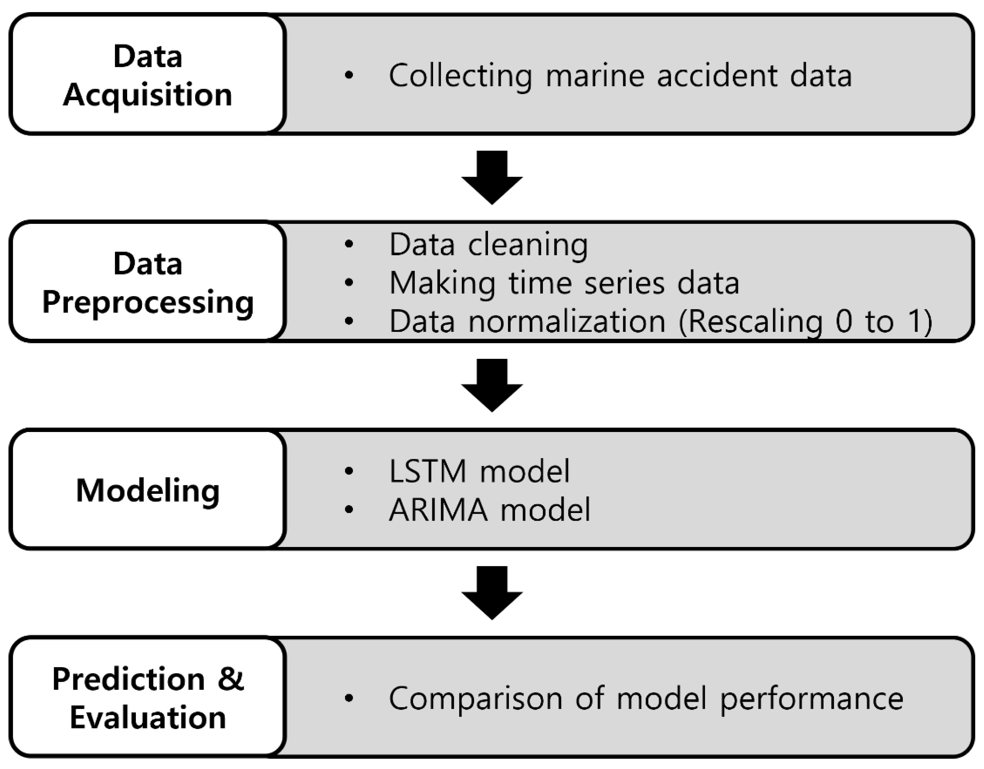
The remainder of the paper is organized as follows: We first describe how the data were collected and preprocessed for this study. Next, the prediction model and the research methodology utilized in this study are presented, followed by the results. Lastly, the findings and implications of this study are discussed.

2. Materials and Methods

In this section, we presented the workflow for our approach to predicting the frequency of marine accidents based on LSTM models. Figure 1 illustrates the entire process of this study, including data acquisition, data preprocessing, the development of a prediction model using LSTM and ARIMA, and the evaluation of the model based on the results of the prediction.

2.1. Data Acquisition

2.1.1. Data Mining

Research on marine accident statistics is found in statistical reports published annually by the Korean Maritime Safety Tribunal (KMST) and the Korea Coast Guard (KCG). In this study, we used statistical data on marine accidents that was published by the KMST. We collected data on marine accidents by watch duty time from 1981 to 2020. In this study, we used the accident data that occurred in Korean territorial waters, including the harbor area. Most statistical studies have been conducted in the field of social science. Therefore, it is necessary to develop scientific statistical techniques for marine accident data. Table 1 shows the sample of marine accidents by the types of marine accidents.

2.1.2. Data Preprocessing

Upon collecting the data from KMST statistics, we performed a preprocessing step in order to classify the accident data by a navigator’s watch duty time and remove the unknown data. Table 2 represents the sample of the processed data on marine accidents by watch duty time. In total, 41,163 data of marine accidents from 1981 to 2020 were used for this study.

2.1.3. Data Normalization and Time Series Data

We created a time series data by connecting the number of marine accidents by navigator’s watch duty time for each year, as illustrated in Figure 2a. To avoid the significant gradient updates that can occur when using large values directly to train an LSTM network, we also rescaled the input data from 0 to 1 before training the LSTM model, as shown in Figure 2b.

2.2. Modeling

2.2.1. LSTM Architecture

Based on the refined data, we developed an LSTM network model, an extension of an RNN, to predict the number of marine accidents by watch duty time. While the RNN is proven to be effective in sequence prediction tasks, numerous problems are still associated with its processing of large data sequences [20]. Due to the gradient propagation problem of the recurrent network over many layers, the RNN is challenging with regard to learning the long-term dependence. Hochreiter and Schimdhuber [21] developed the LSTM network to address these concerns. The LSTM network replaces hidden layers with memory cells for modeling long-term dependencies. Figure 3 illustrates the LSTM architectures.
LSTM models were implemented using Keras libraries in Python, and Tensorflow as the backend in the Spyder tool for Python. We initialized weights and biases for each layer using random values. The LSTM consists of forget gate ( F t ), input gate ( I t ), cell state ( C t ), and output gate ( O t ), which stores information in memory cells and transfers it to the next stage. The forget gate determines how much past information will be forgotten, and it is the process of applying the sigmoid function after multiplying the current data and the hidden layer values of the past by each weight. The input gate controls new information in the cell based on how important the information is. The cell state forgets the past information as calculated by the forget gate and calculates the current memory cell value by multiplying the current information value by the importance of the input gate. Finally, the output gate determines how the information in the cell will be used in the output cell. Each cell contains weights that are used to control each gate. Optimization of the weights is performed by a training algorithm based on an error resulting from network output [24,25]. The mathematical expression of the forget gate ( F t ), input gate ( I t ), cell state ( C t ), and output gate ( O t ) are defined in Equations (1)–(4) [23]:
F t = s i g m o i d ( W x f X t + W h f H t 1 + b f )
I t = s i g m o i d ( W x i n X t + W h i n H t 1 + b i n )
C t = F t C t 1 + I t   ·   t a n h ( W x c X t + W h c H t 1 + b c )
O t = s i g m o i d ( W x o u t X t + W h o u t H t 1 + b o u t )
where t is different time steps, X t represents the t-th observations of variables, t a n h denotes the hyperbolic tangent function, W and b are the parameters of the LSTM network, and H t is the output of the LSTM, which is defined in Equation (5) [23]:
H t = O t   ·   t a n h ( C t )
In this study, we used the LSTM models with one and two hidden layers and one output layer, since the time series data covered in this paper is relatively simple. The number of LSTM units and the number of Time Steps of input data in the hidden layer are optimized. The output layer is composed of a dense layer which is a fully connected layer.

2.2.2. Hyperparameter Tuning for LSTM Model

This study required tuning the hidden units and number of layers of hyperparameters separately for each model to determine the optimal network structure. First, we separated our data into training and test sets. For the training set, we used statistics on marine accidents from 1981 to 2019, and statistics on marine accidents in 2020 were used for the test set. In order to observe how well the network structure is learning, the training set was further divided into 80% training data and 20% validation data. Validation of the prediction model was conducted using the test set. In addition to the use of the validation set, we also used an early stopping strategy that stops training when there was no improvement in the validation metric to avoid an overfitting issue [26]. Input variables that affect learning and accuracy of the LSTM models include the number of layers in the hidden layer, the number of nodes in each hidden layer, activation functions, optimizers, batch size and epoch size. Finding suitable hyperparameter values used in algorithms is of paramount importance in model design for performance optimization of the LSTM models. The hyperparameter tuning process has no fixed method, and the best hyperparameter can be found through an empirical study. Hyperparameters do not have the absolute best values, but they can find suitable values depending on the data and model used. We tuned hyperparameters, such as the number of layers, number of nodes (i.e., hidden units), epoch size, and batch size, using the automated tuning package in Keras [27]. The other input variables we used in this study were as follows:
  • Time steps: This is the number of observations required by the model as inputs to make a future prediction. We set the time steps as six for this study since we divided time into six time periods based on the navigators’ watch duty time.
  • Activation function: This determines the output of the model and serves to transfer the calculation result by the weight to the next layer. We used a hyperbolic tangent, which is commonly used as the activation function [28].
  • Loss function: The mean squared error (MSE) method was used for loss function in this study. The error on the predicted value is expressed in numbers, and the larger the errors, the larger the values, and vice versa.
  • Optimizer: This is used to update the network parameters to minimize loss functions. We chose the Adam optimizer which has the advantage of reducing the load of computational memory [29]. The Adam, which is short for adaptive moment estimation, is an algorithm for the optimization technique for gradient descent. The Adam optimization algorithms have been widely adopted in computer vision and natural language processing applications as an extension to stochastic gradient descent. In order to update network weights iteratively based on training data, the Adam can be used instead of conventional stochastic gradient descent [29].
  • Batch size: This determines the size of the data to be learned at each training stage, and in this paper, it was empirically determined by examining the effect of batch size of 32, 64, 128, 256, and 512 on the prediction performance for all four LSTM networks.
  • Epoch: This is the number of repetitive learnings for the entire training data by batch size. The best epoch we used in this study is 100, which was determined by applying different epoch sizes of 50, 100, 200, 300, 400, and 500.

2.2.3. ARIMA Model

The ARIMA model, developed by Box and Jenkinson in 1970 [30], combines autoregressive (AR) and moving average (MA) models. Since it requires the stationary time series, differencing (integrating) the time series is necessary. Using the Augmented Dickey-Fuller (ADF) [31] unit-root test, we can determine whether or not the time series is stationary. The ARIMA model is represented as ARIMA (p,d,q) with three parameters, such as the order of AR (p), the degree of differencing (d), and the order of MA (q). We estimated the parameters of the ARIMA model using a graph of the autocorrelation function (ACF) and a correlogram of partial autocorrelation (PACF). We chose the best ARIMA model using an automated function in the pmdarima package [32], which utilizes a stepwise approach to search multiple combinations of p, d, and q parameters. The statistical significance level for the ARIMA model was set at 0.05. An Akaike information criterion (AIC), which is an extensively used measure in the evaluation of ARIMA models, was used to evaluate the ARIMA model. It measures the goodness of fit of the model as well as the simplicity of the model. The AIC is defined as:
AIC = 2 l n L ( θ ) + 2 p
where L ( θ ) is the likelihood of the model evaluated at the maximum likelihood estimate (MLE), p is the total number of parameters, and n is the number of observations. Lower AIC values indicate a better model fit.

2.2.4. Performance Evaluation Criteria

To evaluate the learning ability of the LSTM models, in this study, the loss function was used and the most commonly used MSE method was selected among the loss functions. The mean absolute error (MAE) method was used as a metric to measure the accuracy of LSTMs. The MAE is the average of the absolute value between the predicted value and the actual value. In addition, we used mean absolute percentage error (MAPE) to measure the performance of the LSTM and ARIMA models. The MAPE is used to estimate the prediction accuracy of the proposed LSTM and ARIMA models. The MAPE is one of the typical accuracy metrics for time series forecasts. Since the MAPE varies between 0 and 1, we can judge how good the prediction is irrespective of the scale of the series. The error values of these criteria show higher accuracy as the values approach 0. The MSE, MAE, and MAPE are defined as:
MSE = 1 n 1 n ( y y ^ ) 2
MAE = 1 n 1 n | y y ^ |
MAPE = 1 n 1 n | y y ^ y |
where, y and y ^ are the actual value and the predicted value for the frequency of marine accidents, respectively.

3. Results

3.1. Hyperparameter Tuning Results for LSTM

In this study, we built four different LSTM models to see which LSTMs performed best for our data as follows: (1) One LSTM layer with 64 hidden units (LSTM1), (2) Two LSTM layers and 128 hidden units (LSTM2), (3) Two LSTM layers with 64 hidden units (LSTM3), and (4) Two LSTM layers with 256 hidden units (LSTM4). To achieve the best results in terms of prediction accuracy and error, we performed hyperparameter tuning steps for our models. We trained our LSTM models with 100 epochs and the best hyperparameters were tuned by using a function GridSearchCV [33] which is an automated tuning method in the Scikit-learn library in Python. Figure 4, an example of the parameter tuning procedure in the LSTMs, illustrates that loss and MAE for training and validation were identified through 100 epochs. Table 3 shows the best hidden units by the hyperparameter tuning results based on the smallest MAPEs for each LSTM model. The other parameters, such as batch size, epoch size, and the number of layers were also selected in the same way. Table 4 summarizes the list of the best selected hyperparameters for all four models based on our empirical study. Table 5 shows the results of the best loss and MAE for training and validation among 100 epochs.

3.2. ARIMA Results

Marine accident data from 1981 to 2019 were used as a training dataset to develop an ARIMA prediction model. Based on the results of the ADF test, the training dataset was not stationary (p = 0.99). ARIMA (2,1,3) was selected as the best ARIMA model for marine accident forecasting since it had the lowest AIC (AIC = −833.107). Table 6 shows the results of the AIC values of different ARIMA models. The best ARIMA model (i.e., ARIMA (2,1,3)) performed well in the process of testing (MAPE = 0.089). Figure 5 represents the prediction results of the ARIMA (2,1,3) model showing the comparison between actual and predicted values for the testing data.

3.3. Prediction Results for LSTM

With the LSTM models trained using the data from 1981 to 2019, we predicted the number of marine accidents for the marine accidents in 2020 for testing the models. The prediction results for each model are shown in Figure 6 and Table 7. We also calculated the MAPE for each model summarized in Table 7 and then compared the results to find the best model for predicting the frequency of marine accidents by navigator’s watch duty time for 2020. We found that the LSTM3 performed best among the four models (MAPEs for: LSTM3 (0.059) > LSTM4 (0.065) > LSTM1 (0.066) > LSTM2 (0.076).

4. Discussion

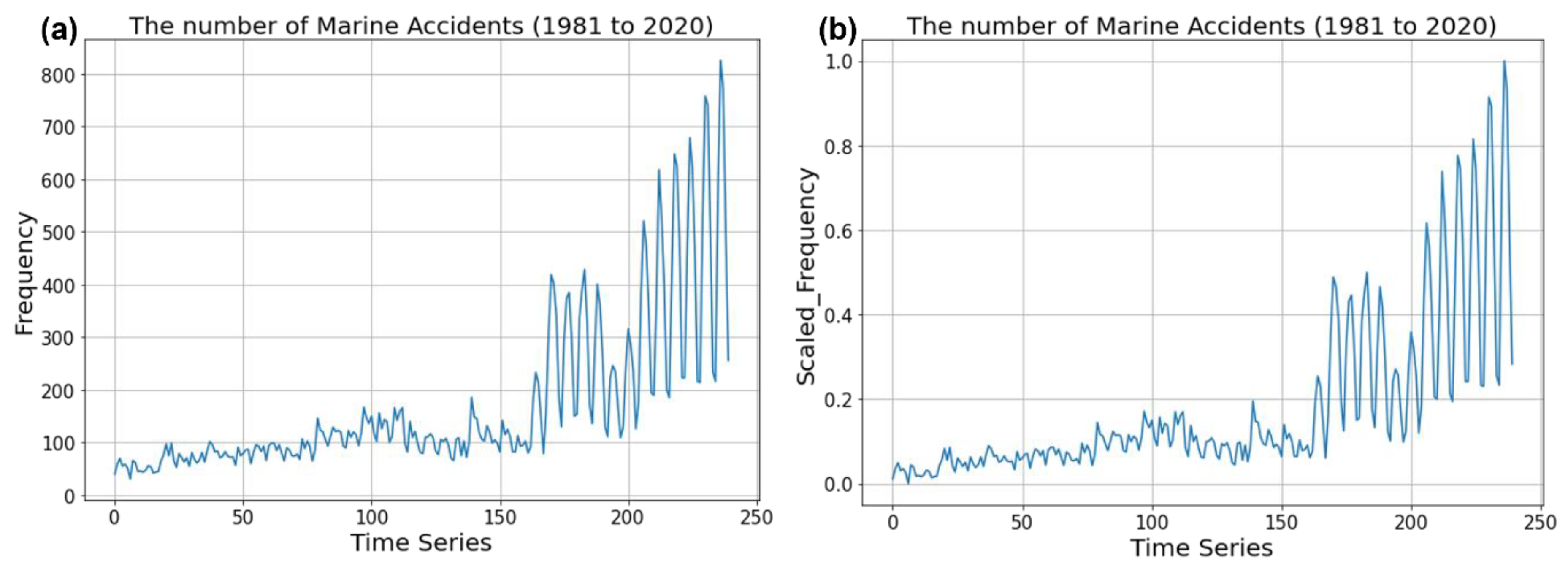
Many researchers studied the prediction of the number of marine accidents, but no research was conducted on the prediction of marine accidents according to the navigator’s duty time. In addition, existing studies related to predicting the number of marine accidents have been conducted via different methods. However, studies related to deep learning, such as LSTM, have been relatively insufficient. To the best of our knowledge, this was the first attempted study to predict the number of marine accidents using LSTM. In this study, marine accidents that occurred in Korea over the past 39 years from 1981 to 2019 were classified by navigator’s duty time, and the number of marine accidents by duty time in 2020 was predicted through the LSTM model. The prediction results were compared with the actual number of marine accidents in 2020.
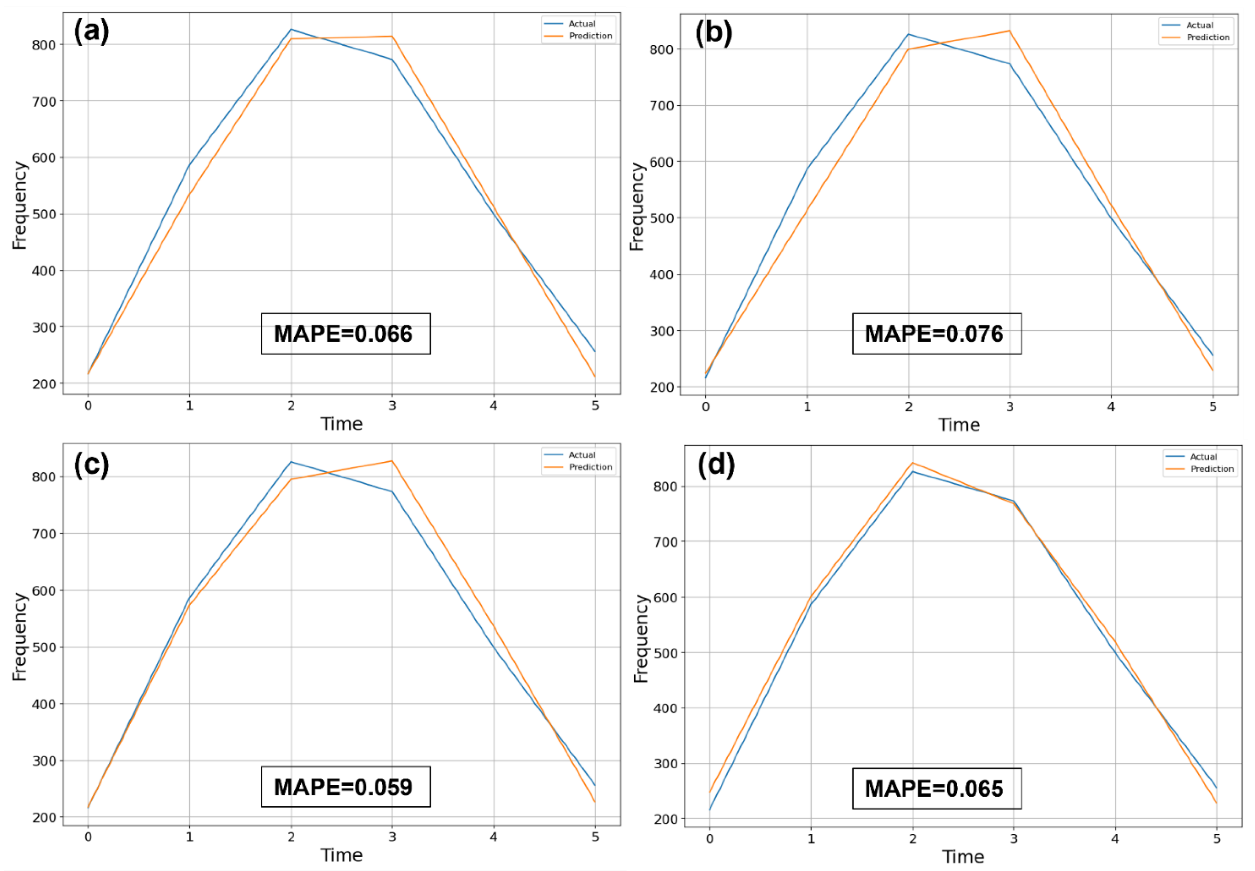
This study showed that the number of marine accidents by the navigator’s watch duty time can be predicted using LSTM through time series data. As a result of comparing the number of marine accidents predicted using the LSTM model with the actual number of marine accidents by duty time in 2020, the proposed LSTM models performed reliably. The MAPEs for all four LSTM models were less than 0.1, which means that the accuracies of the proposed LSTMs were greater than 90%. The best LSTM model was LSTM3, with the smallest MAPE, as shown in Table 7. We found that two LSTM layers (i.e., LSTM3 (MAPE = 0.059) and lSTM4 (MAPE = 0.065)) performed better than a single LSTM layer (i.e., LSTM1 (MAPE = 0.066) and LSTM2 (MAPE = 0.076)). In terms of the effect of hidden units, we noticed that 64 hidden units were better than 128 or 256 hidden units. In addition, the best batch size for each model varied from 18, 24, 30, and 6, respectively. These results can help us guide in the building of a more complex LSTM network structure for our future studies.
To explore the advantage of the LSTM models, we also implemented an ARIMA model, which is a traditional statistical algorithm for time series forecasts. We also compared the performance results of the LSTMs with the ARIMA model. It was shown that all LSTMs outperformed the ARIMA model (MAPE = 0.089). This result proved the superiority of LSTM compared to the ARIMA. Thus, we can say that the LSTM is better than the ARIMA at predicting the frequency of marine accidents by watch duty hours.
Nevertheless, this study still has several limitations. First, although we tuned several hyperparameters, there are more hyperparameters that could significantly affect the performance of the LSTM models. Also, the application of various deep learning algorithms in marine accident prediction models other than LSTM is required. However, since this study is the first attempt to make marine accident predictions using deep learning technology, it can be a guideline when making a complex model for forecasting marine accidents in the future. In addition, this study only used data on the frequency of marine accidents, as this is a univariate time series forecasting study which only uses the previous values of the time series to predict its future values. No other factors were included in this study. Regardless, it is necessary to expand the prediction scope of marine accidents by using time series data with different variables such as weather, human errors, traffic density, and mechanical defects that may be involved in marine accidents. Since this study is a leading study in predicting accidents using deep learning, we believe that it can be a stepping-stone to the study of complex accident prediction models in the future. Lastly, predicting accident frequency does not help prevent it directly. However, by predicting the number of accidents by watch duty time, the pattern of accidents can be learned, and, in fact, most of the accidents occurred during the daytime. This might be because most fishing boats returned in the morning from night fishing and most of the cruise ships and passenger ships that come and go between land and islands were operated during the daytime. Furthermore, many accidents occurred during the watch time of junior officers. On the basic premise that the frequency of marine accidents changes according to the navigator’s experience, it is possible to establish customized accident prevention measures by time by identifying whether the actual marine accidents are concentrated during the junior officer’s duty time. Thus, it is also necessary to reflect the trend of accidents according to these duty hours in the marine accident reduction policy. Using the results, we will be able to help prevent accidents in advance if we make VTS or coast guard officers pay more attention during the time when accidents occur the most. Further study is needed to address these limitations in the future.

5. Conclusions

Marine accidents cause human, material, and environmental damage. In order to minimize the damage caused by the occurrence of an accident, it is necessary to respond to the accident as soon as possible. In other words, if it is possible to predict the approximate time when many marine accidents occur, the department in charge of responding to marine accidents will be able to prevent the spread of additional damage caused by marine accidents by preparing in advance. In this study, we developed the prediction model of the frequency of marine accidents using the LSTM. The proposed LSTM models reliably predicted the number of marine accidents compared to another traditional statistical method, the ARIMA model.
In terms of academic implications, this study could be used for the basis of deep learning approaches for marine accident prediction. In terms of industrial implications, this study could help develop technologies for marine accident prediction and can be used to prevent accidents in industries engaged in maritime safety, such as VTS or the coast guard. The results of this study are expected to be used as basic data to prevent the spread of additional damage by predicting the number of marine accidents by duty time of the navigator and responding early in the event of marine accidents. Although the number of marine accidents can be predicted, it is still insufficient to utilize it to prevent marine accidents in advance. Therefore, future studies will predict marine accidents and propose a model to prevent marine accidents in advance based on the results of this study.

Funding

The APC was funded by the project entiltled “Maritime Safety Audit for Offshore Windfarm in Anma Island, Yeonggwang”.

Institutional Review Board Statement

Not applicable.

Informed Consent Statement

Not applicable.

Data Availability Statement

Not applicable.

Acknowledgments

The author thanks Yu-Min Kwon for his help and support during data collection.

Conflicts of Interest

The author declares that they have no conflict of interest.

References

  1. Ohn, S.-W.; Kwon, Y.-M.; Choi, J. A Study on the Improvement of Vessel Traffic Control of Korean Port in Restricted Visibility. Korean Assoc. Marit. Police Sci. 2021, 11, 145–165. [Google Scholar] [CrossRef]
  2. Park, J.Y. A Study on the Advancement of Maritime Search and Rescue. Korean Assoc. Marit. Police Sci. 2011, 1, 27–54. [Google Scholar]
  3. Korean Maritime Safety Tribunal (KMST). Statistics of Marine Accidents. 2021. Available online: http://www.kmst.go.kr/eng/page.do?menuIdx=227 (accessed on 16 November 2022).
  4. Jang, E.J. A Study on the Prediction of the Frequency of Marine Accidents Using Markov Chain. J. Korean Marit. Police Sci. 2020, 10, 145–170. [Google Scholar] [CrossRef]
  5. Jang, W.J.; Keum, J.S. An Analysis on the Models of Occurrence Probability of Marine Casualties. J. Korean Soc. Mar. Environ. Saf. 2004, 10, 29–34. [Google Scholar]
  6. Park, B.S.; Ahn, Y.S. Statistical analysis of marine accidents by ANOVA. J. Korean Soc. Mar. Environ. Saf. 2007, 13, 191–198. [Google Scholar]
  7. Lee, H.K.; Chang, S.R.; Park, Y.S. A fundamental study on advanced VTS system through statistic analyzing traffic accidents in VTS area. J. Navig. Port Res. 2009, 33, 519–524. [Google Scholar] [CrossRef]
  8. Wang, S.; Yin, J.; Khan, R.U. The multi-state maritime transportation system risk assessment and safety analysis. Sustainability 2020, 12, 5728. [Google Scholar] [CrossRef]
  9. Hänninen, M. Bayesian networks for maritime traffic accident prevention: Benefits and challenges. Accid. Anal. Prev. 2014, 73, 305–312. [Google Scholar] [CrossRef]
  10. Yim, J.B. Analysis of Seafarers’ Behavioral Error on Collision Accidents. J. Navig. Port Res. 2019, 43, 237–242. [Google Scholar]
  11. Oh, J.; Yoon, I.; Hwang, J.; Choi, J.; Han, E. A comparative study of the performance of the traffic accident prediction model at the intersection of the four districts using nonlinear regression analysis, artificial neural network, and structural equation. J. Korean Traffic Assoc. 2014, 32, 266–279. [Google Scholar]
  12. Rye, J.D.; Park, S.; Park, S.; Kwon, C.; Yun, I. A study for development of expressway traffic accident prediction model using deep learning. J. Korean Inst. Intell. Trans. Syst. 2018, 17, 14–25. [Google Scholar] [CrossRef]
  13. Ren, H.; Song, Y.; Liu, J.; Hu, Y.; Lei, J. A Deep Learning Approach to the Prediction of Short-Term Traffic Accident Risk. arXiv 2017, arXiv:1710.09543. [Google Scholar]
  14. Pan, G.; Fu, L.; Thakali, L. Development of a global road safety performance function using deep neural networks. Int. J. Transp. Sci. Technol. 2017, 6, 159–173. [Google Scholar] [CrossRef]
  15. Benoit, F. Road Accidents in Switzerland Forecasting-A Brief Comparison between Facebook Prophet and LSTM Neural Networks. Towards Data Science. 2019. Available online: https://towardsdatascience.com/road-accidents-in-switzerland-forecasting-a-brief-comparison-between-facebook-prophet-and-lstm-6514f585681 (accessed on 16 November 2022).
  16. Sameen, M.; Pradhan, B. Severity prediction of traffic accidents with recurrent neural networks. Appl. Sci. 2017, 7, 476. [Google Scholar] [CrossRef] [Green Version]
  17. Roh, Y.J.; Bae, S.H. Forecasting of Traffic Accident Occurrence Pattern Using LSTM. J. Korean Inst. Intell. Trans. Syst. 2021, 20, 59–73. [Google Scholar] [CrossRef]
  18. Atak, Ü.; Arslanoğlu, Y. Machine learning methods for predicting marine port accidents: A case study in container terminal. Ships Offshore Struct. 2021, 1–8. [Google Scholar] [CrossRef]
  19. Kim, J.H.; Kim, J.; Lee, G.; Park, J. Machine learning-based models for accident prediction at a Korean container port. Sustainability 2021, 13, 9137. [Google Scholar] [CrossRef]
  20. Ullah, A.; Muhammad, K.; Hussain, T.; Baik, S.W. Conflux LSTMs network: A novel approach for multi-view action recognition. Neurocomputing 2021, 435, 321–329. [Google Scholar] [CrossRef]
  21. Hochreiter, S.; Schmidhuber, J. Long short-term memory. Neural Comput. 1997, 9, 1735–1780. [Google Scholar] [CrossRef]
  22. Crisóstomo de Castro Filho, H.; Abílio de Carvalho Júnior, O.; Ferreira de Carvalho, O.L.; Pozzobon de Bem, P.; dos Santos de Moura, R.; Olino de Albuquerque, A.; Rosa Silva, C.; Guimarães Ferreira, P.H.; Fontes Guimarães, R.; Trancoso Gomes, R.A. Rice Crop Detection Using LSTM, Bi-LSTM, and Machine Learning Models from Sentinel-1 Time Series. Remote Sens. 2020, 12, 2655. [Google Scholar] [CrossRef]
  23. Bouktif, S.; Fiaz, A.; Ouni, A.; Serhani, M.A. Optimal Deep Learning LSTM Model for Electric Load Forecasting using Feature Selection and Genetic Algorithm: Comparison with Machine Learning Approaches. Energies 2018, 11, 1636. [Google Scholar] [CrossRef] [Green Version]
  24. Hosseini, M.-P.; Lu, S.; Kamaraj, K.; Slowikowski, A.; Venkatesh, H.C. Deep learning architectures. In Deep Learning: Concepts and Architectures; Springer: Berlin/Heidelberg, Germany, 2019; pp. 1–24. [Google Scholar]
  25. Yu, Y.; Si, X.; Hu, C.; Zhang, J. A review of recurrent neural networks: LSTM cells and network architectures. Neural Comput. 2019, 31, 1235–1270. [Google Scholar] [CrossRef] [PubMed]
  26. Bengio, Y. Practical recommendations for gradient-based training of deep architectures. In Neural Networks: Tricks of the Trade; Springer: Berlin/Heidelberg, Germany, 2012; pp. 437–478. [Google Scholar]
  27. Ketkar, N. introduction to keras. In Deep Learning with Python, 1st ed.; Apress: Berkely, CA, USA, 2017; pp. 97–111. [Google Scholar]
  28. Namin, A.H.; Leboeuf, K.; Muscedere, R.; Wu, H.; Ahmadi, M. Efficient hardware implementation of the hyperbolic tangent sigmoid function. In Proceedings of the 2009 IEEE International Symposium on Circuits and Systems, Taipei, Taiwan, 24–27 May 2009; pp. 2117–2120. [Google Scholar]
  29. Kingma, D.P.; Ba, J.L. Adam: A Method for Stochastic Optimization. In Proceedings of the International Conference on Learning Representations 2015, San Diego, CA, USA, 7–9 May 2015; pp. 1–15. [Google Scholar]
  30. Box, G.E.P.; Jenkins, G.M. Time Series Analysis: Forecasting and Control/Holden Day, San Francisco, California, 1970; John Wiley & Sons: Hoboken, NJ, USA, 2015. [Google Scholar]
  31. Cao, S.; Wang, F.; Tam, W.; Tse, L.A.; Kim, J.H.; Liu, J.; Lu, Z. A hybrid seasonal prediction model for tuberculosis incidence in China. BMC Med. Inform. Decis. Mak. 2013, 13, 56. [Google Scholar] [CrossRef] [PubMed]
  32. Smith, T.G. Pmdarima: ARIMA Estimators for Python. 2017. Available online: http://www.alkaline-ml.com/pmdarima (accessed on 27 October 2022).
  33. Scikit-Learn (Version 1.1.3) Sklearn.Model_Selection.GridSearchCV. Available online: https://scikit-learn.org/stable/modules/generated/sklearn.model_selection.GridSearchCV.html (accessed on 27 October 2022).
Figure 1. Workflow for predicting the frequency of marine accidents.
Applsci 12 11724 g001
Figure 2. Time series of marine accidents from 1981 to 2020 for: (a) original data; (b) rescaled data.
Applsci 12 11724 g002
Figure 3. Architectures of the LSTM layer [22,23].
Applsci 12 11724 g003
Figure 4. Hyperparameter tuning process for each LSTM model. Loss and MAE values of training and validation for: (a) LSTM1, (b) LSTM2, (c) LSTM3, and (d) LSTM4.
Applsci 12 11724 g004
Figure 5. Prediction results of ARIMA (2,1,3) model (MAPE = 0.089). The blue line represents training data, and the orange and green lines represent actual and forecasted values, respectively.
Applsci 12 11724 g005
Figure 6. Prediction results with test data (marine accidents by watch duty time in 2020) for each LSTM: (a) LSTM1 (MAPE = 0.087), (b) LSTM2 (MAPE = 0.107), (c) LSTM3 (MAPE = 0.076), and (d) LSTM4 (MAPE = 0.133). The numbers 0 to 5 in the time axis represent the navigator’s watch duty time 00–04, 04–08, 08–12, 12–16, 16–20, and 20–24, respectively. Blue and orange lines represent actual and predicted values, respectively.
Applsci 12 11724 g006
Table 1. Sample of collected raw data.
YearTypes of Marine AccidentsTotal
CollisionContactGroundingCapsizingFireSinkingEngine FailureCasualtyOthers
1981171575752022451826421
1982160355521016482225373
1983130304931029542334362
19841503367816431464053556
1985184306171966821339501
2019244 38 140 110 132 61 888 228 11302971
2020277 39 198 108 128 69 878 203 12563156
Table 2. Sample of processed data.
YearFrequency of Marine Accidents by Watch Duty TimeTotal
0–44–88–1212–1616–2020–24
1981405970555951334
1982316662454644294
1983475654424445288
1984657697759965477
1985537972637155393
20192145257587414992342971
20202165868267734992563156
Table 3. The best hyperparameter for hidden units. Hidden units for LSTM1 to LSTM4 were selected as 64, 128, 64, and 256, respectively. * represents the smallest MAPE values for each model.
Hidden UnitsMAPE
LSTM1LSTM2LSTM3LSTM4
320.1060.0980.1200.137
640.094 *0.1100.066 *0.079
1280.0990.095 *0.0770.096
2560.1030.1010.1050.065 *
5120.0980.0990.0870.084
Table 4. List of the best selected hyperparameters for each LSTM model using GridSearchCV. We fixed the time steps, learning rate, and optimizer in this study.
ModelLSTM LayerHidden UnitsTime StepsBatch SizeLearning RateEpochOptimizer
LSTM11646180.0001100Adam
LSTM211286240.0001100Adam
LSTM32646300.0001100Adam
LSTM42256660.0001100Adam
Table 5. Results of loss and MAE for training and validation. The loss and MAE values in the table were the best values among 100 epochs.
ModelLossMAE
TrainingValidationTrainingValidation
LSTM10.00210.00180.03000.0351
LSTM20.00240.00240.03180.0298
LSTM30.00290.00090.03420.0276
Table 6. Comparison of the ARIMA models. ARIMA (2,1,3) was selected as the best model with the lowest AIC.
ModelAICModelAIC
ARIMA (0,1,0)−390.901ARIMA (2,1,1) −743.474
ARIMA (0,1,1) −492.557ARIMA (2,1,2) −813.302
ARIMA (1,1,0) −435.452ARIMA (2,1,3) −833.107
ARIMA (1,1,1) −495.050ARIMA (3,1,0) −723.283
ARIMA (1,1,2) −548.133ARIMA (3,1,1) −776.187
ARIMA (1,1,3) −595.263ARIMA (3,1,2) −777.236
ARIMA (2,1,0) −629.584ARIMA (3,1,3) −824.376
Table 7. Comparison of prediction results of four different LSTM models with the ARIMA model. LSTM3 has the smallest MAPE (0.059). Except for LSTM2, all other LSTM models outperformed the ARIMA model.
ModelValueThe Number of Marine Accidents by Watch Duty TimeMAPE
00–0404–0808–1212–1616–2020–24
-Actual216586826773499256-
LSTM1Predicted2165348098145122120.066
LSTM2Predicted2245137998325232290.076
LSTM3Predicted2175737958285362260.059
LSTM4Predicted2476018427685192280.065
Publisher’s Note: MDPI stays neutral with regard to jurisdictional claims in published maps and institutional affiliations.

