Distinction of Scrambled Linear Block Codes Based on Extraction of Correlation Features

Abstract

Aiming to solve the problem of the distinction of scrambled linear block codes, a method for identifying the scrambling types of linear block codes by combining correlation features and convolution long short-term memory neural networks is proposed in this paper. First, the cross-correlation characteristics of the scrambling sequence symbols are deduced, the partial autocorrelation function is constructed, the superiority of the partial autocorrelation function is determined by derivation, and the two are combined as the input correlation characteristics. A shallow network combining a convolutional neural network and LSTM is constructed; finally, the linear block code scrambled dataset is input into the network model, and the training and recognition test of the network is completed. The simulation results show that, compared with the traditional algorithm based on a multi-fractal spectrum, the proposed method can identify a synchronous scrambler, and the recognition accuracy is higher under a high bit error rate. Moreover, the method is suitable for classification under noise. The proposed method lays a foundation for future improvements in scrambler parameter identification.

1. Introduction

In communication systems, a long 0-run or 1-run often appears in transmitted binary sequences [1], and this affects the extraction of timing information in signals. To improve the balance of 0 and 1 symbols in transmitted signals, transmitted signals are scrambled to make it nearly completely random digital sequences [2]. Scrambling processing enhances the reliability and security of signal transmission, so it is widely used in satellite communications, spread spectrum communications, and cryptography [3,4,5]. In non-cooperative communication, the extraction of scrambled information must be descrambled first, so the blind identification technology of scrambling code parameters is of great significance to the extraction of non-cooperative information and the deciphering of ciphers [6,7].

A scrambling code is divided into a synchronous scrambling code and a self-synchronous scrambling code [6,7]. Among these, the parameter identification of the synchronous scrambling code is the identification of a generator polynomial and the initial state, and the identification of the self-synchronous scrambling code is the identification of a generator polynomial. In recent years, scrambling code parameter identification technology has been widely studied [6,7]. The methods of scrambling parameter identification mainly focus on three types of situations: source unbalance [8,9,10,11,12,13,14,15,16], source balance (coding scrambling) [17,18,19,20,21], and the estimation of scrambled sequences in a direct-sequence spread spectrum [22,23,24,25].

In an actual communication system, signal transmission is often channel-coded, so intercepted scrambled data are usually a source-unbalanced sequence that has been channel-coded and then scrambled. A method for reconstructing the synchronous scrambling code generator polynomial based on a dual code and double search was proposed by Liu [17], in which one must know the scrambling type; in addition, the detection performance index always meeting the requirements cannot be maintained. In [18], a more robust sparse double-search algorithm, which improved the recognition performance of the algorithm under a low signal-to-noise ratio, was put forward. However, knowledge of the constraint length of the encoding is required. In [19], a polynomial identification based on run-length statistics was proposed to solve the self-synchronous scrambling of linear block codes. This method does not require prior information, and the influence of bit errors and channel noise is also not considered. The cost function of a generator polynomial based on the known check vector of the dual code was constructed in [20], and the reconstruction of the generator polynomial under the noisy condition of the convolutional code was completed. The third-order correlation of a synchronously scrambled m-sequence was used in [21] to complete the reconstruction of a generator polynomial under error conditions. This method does not require the information of an a priori vector, nor does it consider the influence of channel noise, but it requires the known coding of the constraint length.

From the above analyses, all the known scrambling code parameter identification methods are based on the known channel coding and scrambling types, but the scrambling code data intercepted by non-cooperative communication parties are unknown, so it is necessary to analyze whether the outgoing signal is scrambled and what scrambling method is adopted that can further identify the parameters. Based on this, a multitype spectrum classification method, which solved the binary classification of linear block codes and linear block code self-synchronous scrambling under error conditions, was proposed in [26]. However, since the biased difference between linear self-synchronous scrambling and linear synchronous scrambling is very small, the distinction between the two leads to poor classification performance. At the same time, the influence of channel noise and recognition performance under high error conditions must be further improved. Reference [21] constructed a rank difference matrix, and when different scrambling methods were used, there was a periodic loss of rank at the integer multiples of the code length, which was used as a basis to judge the scrambling method. Reference [27] proposed to apply neural networks in order to extract rank features for the purpose of classification. However, the structure and parameters of the neural network were not given. Meanwhile, when the BER is greater than 0.01, the matrix tends to be a random matrix, the rank feature is not obvious, and the recognition rate tends to be 0. To summarize, due to the need for accurate scrambling-type information, the existing algorithms cannot achieve the full blind identification of linear block code scrambling. In recent years, deep learning methods have achieved good results in signal recognition [28,29], modulation recognition [30,31], malicious file detection [32,33], and other fields [34,35]. At the same time, deep-learning-based methods avoid manual feature extraction and have high practical value.

To solve the above-mentioned problems and the difficulty of manual feature extraction, under the conditions of a high bit error rate (BER) and a low signal-to-noise ratio (SNR), in this paper, we propose a linear block code scrambling-type identification based on correlation feature extraction. The contributions of this paper are summarized as follows:

(1) We deduce the symbol cross-correlation of the scrambling sequence and construct the partial autocorrelation function, both of which can reflect the correlation characteristics of different scrambling methods.

(2) We construct a shallow network consisting of convolutional neural network (CNN) and long short-term memory (LSTM) neural network models, which can accomplish the identification of scrambled linear block codes under a high BER and a low SNR.

The remainder of this paper is organized as follows: In Section 2, we summarize the principle and mathematical model of the scrambler. In Section 3, we analyze the cross-correlation characteristics of the symbols and construct a partial autocorrelation function. A correlation feature extraction network model is built in Section 4, and we analyze the training process of the network. In Section 5, the proposed method is evaluated using Monte Carlo simulations, and we compare its performance with that of the multi-fractal spectrum method. Finally, a discussion is provided in Section 6.

2. Scrambled Linear Block Code Model

The basis of the scrambling code is the linear-feedback shift register (LFSR), in which the self-synchronous scrambling code introduces an exclusive OR logic between the feedback logic output and the first-stage register, and the obtained result is used as the input of the register. The independent m-sequence generated by the LFSR is added to the information sequence, thereby generating the scrambling sequence. The self-synchronous scrambler and synchronous scrambler are shown in Figure 1a,b, respectively.

An L-stage LFSR’s feedback network is made up of L registers, such as the first-stage register and the second-stage register, and an L-th stage register from left to right. Each register can have two states, 0 and 1, and the operation $\oplus$ means the addition of modulo-2. When a shift pulse is added, the output content of the previous moment is fed back to the first-level register, the content of each level register is shifted to the next level, and the current output $s_t$ is generated by operation. Therefore, after giving the initial values, $s_0,s_1,\dots ,s_{L-1}$, under the action of the shift pulse, the L-stage LFSR outputs a sequence $\left\{s_t\right\}$, which satisfies the feedback logic

$$s_t=c_1{s}_{t-1}\oplus c_2{s}_{t-2}\oplus \cdots \oplus c_L{s}_{t-L},$$

(1)

where $c_i\in GF\left(2\right),1\le i\le L$. This sequence is called the LFSR sequence, and its linearity is mainly reflected in its feedback logic being linear. Any consecutive L term in a sequence of the L-stage LFSR is called the state of the sequence. $\left(s_0,s_1,\dots ,s_L\right)$ is called the initial state [16].

The self-synchronous scrambling process can be expressed as

$$y_k=x_k\oplus {\displaystyle \sum _{i=1}^L\oplus c_i{y}_{k-i}}.$$

(2)

Additionally, the synchronous scrambling process can be expressed as

$$y_k=x_k\oplus {\displaystyle \sum _{i=1}^L{c}_i{s}_{k-i}},$$

(3)

where $\sum \oplus$ means modulo-2 accumulation. $c_i\in GF(2), i=1,2,\dots ,L$ is the feedback coefficient of the LFSR, $GF(2)$ represents the 2-element domain, and the value of $c_i$ is 0 or 1, $c_0=c_L=1$. The generator polynomial of the scrambling code can be expressed as

$$f(x)=1+c_{1}x+c_2{x}^2+\cdots +c_L{x}^L.$$

(4)

In actual communication system information transmission, most of the sources become unbiased sources through channel coding [17], so the signal model studied in this paper is shown in Figure 2 [17,18].

The noise is Gaussian white noise with mean 0, variance ${\sigma }^2$, and signal amplitude $A$. The signal-to-noise ratio (SNR) is defined as

$$\mathrm{SNR}=10\cdot \log \left(A^2/2{\sigma }^2\right).$$

(5)

For the receiver, first, we intercept a sequence of code elements of a linear block code, and we only need to determine whether the sequence of the code elements is scrambled using LFSR. When scrambling is performed, it is further determined whether the code element sequence employs a self-synchronous scrambler as shown in Figure 1a or a synchronous scrambler as shown in Figure 1b. Further identification of the scrambling parameters is only possible when the above three types of code element sequences are distinguished. In the next section, we focus on how to effectively identify whether the intercepted information sequence is scrambled and what kind of scrambling method is used.

3. Analysis of Correlation Characteristics of Scrambled Linear Block Code

3.1. Cross-Correlation Characteristics of Symbols

It can be seen from Equation (2) that the k-th symbol ($y_k$) of the self-synchronous scrambling sequence correlates with the previous $L$ symbol $\left(y_{k-i}, i=1,2,\dots ,L\right)$ regardless of the state of the LFSR.

It can be seen from Equation (3) that the k-th symbol ($y_k$) of the synchronous scrambling sequence correlates with the first $L$ states $\left(s_{k-i}, i=1,2,\dots ,L\right)$ of the LFSR. The relationship between the kth symbol and the state of the LFSR is

$$y_{k-1}=x_{k-1}\oplus {\displaystyle \sum _{i=1}^L\oplus }{c}_i{s}_{k-i-1}.$$

(6)

Furthermore,

$$s_{k-1}={\displaystyle \sum _{i=1}^L\oplus }{c}_i{s}_{k-i-1}=y_{k-1}\oplus x_{k-1}.$$

(7)

The state of the LFSR at each moment satisfies the following relationship [14]:

$$s_k={\displaystyle \sum _{i=1}^L{c}_i}{s}_{k-i}.$$

(8)

Combining Equations (2) and (6)–(8), it can be deduced that the following correlation exists between the $k$-th symbol and the first $L$ symbol:

$$\begin{array}{ll}{y}_k& =x_k\oplus s_k=x_k\oplus c_1{s}_{k-1}\oplus c_2{s}_{k-2}\oplus \cdots \oplus c_L{s}_{k-L}\\ & =x_k\oplus c_1\cdot \left(x_{k-1}\oplus y_{k-1}\right)\oplus c_2\left(x_{k-2}\oplus y_{k-2}\right)\oplus \cdots \oplus c_L\left(x_{k-L}\oplus y_{k-L}\right)\end{array}$$

(9)

However, when the linear block code is not scrambled, the preceding and following symbols have no correlation with the LFSR, and they are only related to the generator matrix of the linear block code. In summary, the linear block code scrambling correlation distribution is shown in Figure 3.

It can be seen in Figure 3 that there is no correlation between the symbols of the linear block code and the LSFR; there is a correlation between the two symbols of the linear block code self-synchronous scrambling, and the symbols have nothing to do with the state of the LFSR; there is a correlation between the symbol and states of the first L LFSRs at the moment of the synchronous scrambling of the symbols of the linear block code, and, at the same time, this leads to a correlation between the symbols. It can be seen from the above analysis that scrambling causes a correlation between the preceding and following symbols. This correlation is related to the state of the LFSR (synchronous scrambling) or is independent (self-synchronous scrambling), so the intercepted symbol sequence can be used as a correlation feature that is used for linear block code scrambling classification.

3.2. Biased Autocorrelation Characteristics of Symbols

From the analysis in Section 3.1, there are correlation characteristics between the symbols scrambled by the linear block code, and they have relatively good correlation characteristics. Next, the biased autocorrelation function [36] of the symbol sequence is constructed as follows:

$$r_{yy}^{\prime }\left(\tau \right)=\frac{1}{N}{\displaystyle \sum _{k=0}^{N-\tau -1}{Y}_k}{Y}_{k+\tau },\tau \in \left[0,N-1\right].$$

(10)

where $Y_k=1-2y_k$.

The unbiased autocorrelation function is defined as

$$r_{yy}\left(\tau \right)=\frac{1}{N-\tau }{\displaystyle \sum _{k=0}^{N-\tau -1}{Y}_k}{Y}_{k+\tau }.$$

(11)

The relationship between the unbiased and biased autocorrelation functions is expressed as follows:

$$r_{yy}^{\prime }\left(\tau \right)=\frac{N-\tau }{N}{r}_{yy}\left(\tau \right),$$

(12)

where $r_{yy}\left(\tau \right)$ is an unbiased estimate, and the following formula can be obtained:

$$E\left[r_{yy}^{\prime }\left(\tau \right)\right]=\frac{N-\tau }{N}{r}_{yy}\left(\tau \right).$$

(13)

It can be seen from Equation (13) that $r_{yy}^{\prime }\left(\tau \right)$ is a biased estimate but is asymptotically unbiased, and its offset is

$$B=\frac{\tau }{N}{r}_{yy}\left(\tau \right).$$

(14)

The variance of the estimator is

$$var\left[r_{yy}^{\prime }\left(\tau \right)\right]={\left(\frac{N-\tau }{N}\right)}^2\cdot var\left[r_{yy}\left(\tau \right)\right]$$

(15)

It can be deduced that

$$var\left[r_{yy}^{\prime }\left(\tau \right)\right]\le \frac{1}{N}{\displaystyle \sum _{m=1+\tau -N}^{N-\tau -1}[r_{yy}^2\left(m\right)+} r_{yy}\left(m+\tau \right)r_{yy}\left(m-\tau \right)]$$

(16)

When $N\to \infty$, $var\left[r_{yy}^{\prime }\left(\tau \right)\right]\to 0$, and we have

$$var\left[r_{yy}^{\prime }\left(\tau \right)\right]\le var\left[r_{yy}\left(\tau \right)\right].$$

(17)

It can be seen from the above analysis that, although the biased autocorrelation function is biased, it is asymptotically consistent, and the variance in the estimator is smaller than that in the unbiased estimate.

To facilitate comparison and analyses, the biased autocorrelation function is normalized. Under the conditions that the BER is 0.1 and SNR = 6 dB, the normalized partial autocorrelation functions are shown in Figure 4 and Figure 5, respectively.

It can be seen in Figure 4 and Figure 5 that the normalized partial autocorrelation functions of the different scrambling types have different peaks and periodic changes at each moment under the conditions of bit error and noise, so they can be used as another classification feature.

Since it is difficult to manually extract the above features, a method based on a convolutional LSTM neural network is established for feature extraction and training learning.

4. Scrambled Linear Block Code Identification Based on Correlation Features Extraction Network

4.1. Correlation Feature Extraction Network Model

In this paper, the received scrambling sequence features are divided into two lines: one line contains the original symbol sequence of the cross-correlation feature, and the other is the normalized partial autocorrelation function of the sequence; and the two form the $2\times \beta$-dimensional matrix feature as the input of the network.

It can be seen from the analysis in Section 2 that the scrambling sequence has timing-related characteristics. As a special recurrent neural network, LSTM has achieved good results in processing timing-related information [37,38]. In the present study, CNN and LSTM are combined. The structure of the network, which is mainly composed of two convolutional layers, i.e., one LSTM layer and one fully connected layer, is shown in Figure 6. The activation function of the convolutional layer adopts RELU, the activation function of the LSTM layer adopts tanh, the final fully connected layer uses the normalized exponential function (SoftMax) for classification, and the output is a dimensional one-hot encoding form, corresponding to linear block codes, linear block code self-synchronous scrambling, and linear block code synchronous scrambling.

To prevent overfitting, we first introduce a Dropout layer after each layer of the network to randomly drop some neurons in order to reduce the overfitting phenomenon of the network. Moreover, the EarlyStopping function is used to detect the loss value and to stop training when it is not decreasing.

4.2. Network Training Process

The convolution kernel of convolutional layer 1 is 2 × 1. Since the input sample is a sequence of the code elements of the receiver signal and autocorrelation features, which form the real and imaginary parts of the input sample, respectively, the input sample is not the received sequence $z=\left[z\left(0\right),z\left(1\right),\dots ,z\left(k-1\right)\right]$. Therefore, it is necessary to first combine the real and imaginary parts of the scrambled sequence and to then extract the features based on the correlation.

As can be seen in Figure 3, when the 1 × 2-dimensional convolution kernel is used to extract the signal features of the scrambled sequences, the deep features obtained from their convolution must show different patterns due to the different correlations of the linear block code, the self-synchronization of the linear block code, and the synchronization of the linear block code. In fact, the process of the convolution of the received sequence using a 1 × 2-dimensional convolution kernel is similar to the calculation of its correlation features under time delay. However, for the self-synchronization of linear block code and the synchronization of linear block code, the correlation features of code elements separated by more than two code elements are not as obvious as those of two adjacent code elements, so convolutional kernels with lengths longer than 1 × 2 dimensions do not have this differentiation advantage, and they increase the parameters of network training and increase network complexity. Therefore, the 1 × 2-dimensional convolution kernel is used to convolve the layer 1 output features in order to obtain correlation features that are more consistent with the nature of scrambled signals.

The weight and bias training update of the correlation feature extraction network is mainly divided into two processes: forward propagation and back propagation. Among them, the forward propagation process is to use the input training samples in order to calculate the neuron activation value of the network, and the back propagation process is to perform a reverse calculation in order to obtain the gradient corresponding to the weight and bias of each error; finally, the gradient-descent algorithm is used to calculate the weight and to offset update adjustment.

Consider the training data $\left\{\left(y^{\left(1\right)},q^{\left(1\right)}\right),\left(y^{\left(2\right)},q^{\left(2\right)}\right),\cdots ,\left(y^{\left(m\right)},q^{\left(m\right)}\right)\right\}$ with a sample size of $m$, where $y^{\left(\mathrm{i}\right)}(\mathrm{i}=1,2,\dots ,m)$ is the input scrambled data, and $q^{\left(i\right)}\left(i=1,2,\cdots ,m\right)$ is the type label corresponding to the scramble code. The $W$ and $b$ update formulas are, respectively, expressed as follows:

$$W^{t+1}=W^t-\alpha \frac{\partial J\left(W,b;y,q\right)}{\partial W^t},$$

(18)

$$b^{t+1}=b^t-\alpha \frac{\partial J\left(W,b;y,q\right)}{\partial b^t}.$$

(19)

where $\alpha$ is the learning rate, and $J(\cdot )$ is the loss function. The loss function used is categorical_crossentropy, which is a loss function for mul-ticlass classification tasks and is suitable for the multiclass problem.

The expression of $J(\cdot )$ is

$$J\left(W,b;y,q\right)=-\frac{1}{m}{\displaystyle \sum _{i=1}^m{q}^{\left(i\right)}}\cdot \log \left(f\left(W,b;y^{\left(i\right)}\right)\right)+\lambda {{\displaystyle \sum \Vert W\Vert }}^2.$$

(20)

where $\lambda$ is the regularization coefficient used to prevent the network from overfitting.

The input $x_m^{(l)}(j)$ and output $y_m^{(l)}(j)$ of each layer of neurons in the network have the following relationship:

$$y_m^{(l)}(j)=f\left(x_m^{(l)}(j)+b_m^{\left(l\right)}\left(j\right)\right).$$

(21)

where l is the layer number of the network, j is the j-th neuron of the feature map, $m$ is the $m$-th feature map in the network layer number, $f(\cdot )$ is the activation function used by this layer, and $b$ is the bias.

4.3. Input–Output Relationship of Each Network Layer

The input $2\times \beta$ training data are represented as $I_{N,T}$, where $N$ represents the dimension of the two features, and $T$ is the number of sampling points. The input–output relationship of each network layer is detailed as follows:

(1) Input layer:

$$Input=I_{N,T}.$$

(22)

(2) Convolutional layer:

$$y_m^{(2)}(j,k)=f({\displaystyle \sum _{i=1}^3{I}_{j,(k-1)\times 1+i}\times {\ker }_m^{(2)}+b_m^{(2)}(j,k))}.$$

(23)

(3) LSTM layer:

$$h_t=f(W_{hx}{y}_{m,t}^{(3)}(j)+W_{hh}{h}_{t-1}+b_h),$$

(24)

$$h_t^n=f(W_{h^{n-1}{h}^n}{h}_t^{n-1}+W_{h^n{h}^n}{h}_{t-1}^n+b_h^n),$$

(25)

$$y_m^{(4)}(j)=W_{h^{N}y}{h}_t^N+b_y,$$

(26)

where $W_{hx}$ represents the weight matrix between the input layer and the hidden layer, $W_{hh}$ represents the weight matrix between the hidden layers, $h_t$ represents the hidden activation at time $t$, $n\left(n=1,2,\dots ,N\right)$ represents the current network layer, and $h_t^n$ represents the $n$ layer and output at time $t$.

(4) SoftMax layer:

$$y^5(j)=f({\displaystyle \sum _{i=1}^{n_4}{y}^{(4)}(i)\times w^{(5)}(i)}+b^{(5)}(j)).$$

(27)

where $w_i^{(5)}(l)$ represents the connection weight between the fifth and sixth layers, and $n_4$ is the number of neurons in the fifth layer.

The SoftMax layer calculates the probability estimate of the corresponding category in the sample, and the learned hypothesis function $h_{\theta }\left(x\right)$ is expressed as follows:

$$h_{\theta }(y^i)=\left[\begin{array}{c}p(q^{(i)}=1|y^{(i)};\theta )\\ p(q^{(i)}=2|y^{(i)};\theta )\\ \cdots \\ p(q^{(i)}=k|y^{(i)};\theta )\end{array}\right]=\frac{1}{{\displaystyle \sum _{j=1}^k{e}^{{\theta }_j^T{y}^{(i)}}}}.$$

(28)

where ${\theta }_1,{\theta }_2,\dots ,{\theta }_k\in R^{n+1}$ is the model parameter. To simplify the model, we define the function

$$l\{\alpha \}=\{\begin{array}{ll}1,& \alpha =true\\ 0,& \alpha =false\end{array}.$$

(29)

The cost function of the SoftMax layer can be further expressed as

$$J(\theta )=-\frac{1}{m}[{\displaystyle \sum _i^m{\displaystyle \sum _{j=1}^{k}l\{q^{(i)}=j\}\log \frac{e^{{\theta }_j^T{y}^{(i)}}}{{\displaystyle {\sum }_{l=1}^k{e}^{{\theta }_j^T{y}^{(i)}}}}}}.$$

(30)

By superimposing the k values, the probability that the network classifies the scrambled data into the $j$-th category is

$$p(q^{(i)}=j|y^{(i)};\theta )=\frac{e_j^T{y}^{(i)}}{{\displaystyle {\sum }_{l=1}^k{e}_j^T{y}^{(i)}}}.$$

(31)

where the maximum probability corresponds to the classification category of the scrambling code.

We first extract the autocorrelation and the intercorrelation features of the code element data used as input data; compared with the method in [27], the training and learning of the neural network are carried out, and the biggest advantage of a neural network over manually extracting features is that it can learn the training autonomously, so the recognition effect is better than simply manually extracting features. Compared with the method in Reference [26], a detailed neural network model is constructed, but the autocorrelation features and the intercorrelation features extracted in this paper have better anti-BER and noise performance than the matrix rank features in Reference [26]. When the BER is greater than 0.1, the matrix rank features become extremely insignificant because of erroneous code elements, and this leads to weaker features extracted by the neural network. Therefore, the current method in this paper achieves better results.

5. Results

5.1. Experimental Dataset

Two datasets were constructed, i.e., a scrambled dataset of 2000 frames under the condition of bit error (a bit error rate of 2000), and a scrambled dataset of 2000 frames under the condition of white Gaussian noise (with an SNR in the range of 10–15 dB).

During the training process, 80% of the total samples were randomly selected as training data, with the rest used as test data. The datasets and labels are shown in

Table 1. Linear block code scrambling dataset under bit error.

Dataset	Label	Number of Signals	Number of Samples $\left(2\times 400\right)$
linear block code	0	$2000\times 400$	2000
self-synchronous scrambler	1	$2000\times 400$	2000
synchronous scrambler	2	$2000\times 400$	2000

and

Table 2. Linear block code scrambling dataset with noise.

Dataset	Label	Number of Signals	Number of Samples $\left(2\times 800\right)$
linear block code	0	$2000\times 800$	2000
self-synchronous scrambler	1	$2000\times 800$	2000
synchronous scrambler	2	$2000\times 800$	2000

.

The simulation experiment was conducted on an Inteli7-9700K CPU with 16 Gb of memory and an RTX3080 graphics card running Windows 10; the model was built and trained based on TensorFlow.

5.2. Network Model Parameters

Because the Adam optimizer was chosen in this manuscript, the optimizer adaptively adjusts the learning rate, and the automatic learning rate is not a function of epoch. So, there was no need to consider learning rate schedule as a function of epochs. The network model parameters are shown in

Table 3. Network model parameters.

Network Parameters	Numerical Value
batch size	20
learning rate initial value	$1\times {10}^{-4}$
final number of epochs	100
validation part of training set	25% of the training set
initial value of the weight constraint coefficient	0.01
number of LSTM units with shared weights	6

.

5.2.1. Effect of LSTM Layers and Parameters on Recognition Rate

We analyzed the effects of the number of LSTM layers and cells on the recognition rate of the algorithm, as shown in Figure 7 and Figure 8, respectively.

In Figure 7 and Figure 8, we can see that the recognition rate is the highest when the number of LSTM layers is 1, and the recognition results are better when the number of cells is 32 or 68. However, the training time of the network increases a lot when the number of cells is 68, so for the number of cells, 32 was chosen, as it has a shorter training time.

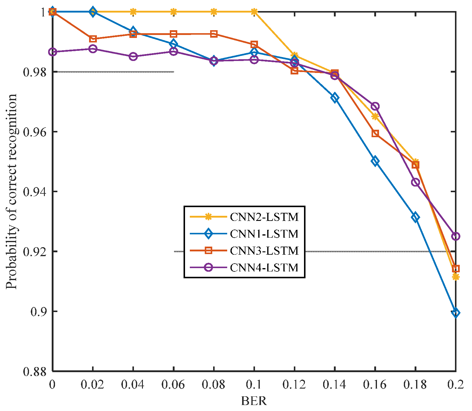
5.2.2. Effect of CNN Layers and Parameters on Recognition Rate

We analyzed the effects of the number of CNN layers and cells on the recognition rate of the algorithm, as shown in Figure 9 and Figure 10, respectively.

As can be seen in Figure 9 and Figure 10, the highest recognition rate is achieved when the number of CNN layers is 2; the recognition effect is better when the number of convolutional layer cells in the first layer is 32, and the number of convolutional layer cells in the second layer is 68.

5.3. Experimental Results

5.3.1. Recognition Rate of The Proposed Algorithm under Bit Error Condition

To verify the validity of the model proposed in this paper, we analyzed the influence of the linear block code parameters, the number of intercepted samples, and the order and terms of the generator polynomial on the network performance under different error conditions.

The relationship between the parameters of the different linear block codes and the recognition rate of the algorithm when the generator polynomial is $f\left(x\right)=1+x^{18}+x^{23}$ and the number of samples is 400 is shown in Figure 11.

It can be seen in the figure that, under the same simulation conditions, the (15,5) linear block code has the highest recognition rate. At that time, the recognition rate under the four coding parameters can reach more than 85%, indicating good anti-error performance.

The (15,5) linear block code scrambling recognition rate under different sample numbers when the generator polynomial is $f\left(x\right)=1+x^{18}+x^{23}$ is shown in Figure 12.

It can be seen in the figure that, under the same error conditions, more samples mean a higher recognition rate of the algorithm. When the number of samples is 100 and the error rate is 0.2, the recognition rate is greater than 80%. When the error rate is 0.1, the recognition rate can reach 98%, which shows that the proposed algorithm has better performance under the conditions of a small number of samples and a high BER.

The (15,5) linear block code scrambling recognition rate under different generator polynomials for 400 samples is shown in Figure 13.

It can be seen in Figure 13 that, with an increase in the bit error rate, the recognition rate gradually decreases. The difference in the recognition rate under a generator polynomial of different orders and terms is not more than 1%. Therefore, the algorithm proposed in this paper is free from the scrambling code generator polynomial order.

The performance of the algorithm proposed in this paper under different linear block code parameters is compared with that of the method proposed in Refs [26,27]. When the generator polynomial is $f\left(x\right)=1+x^{18}+x^{23}$, the number of samples is 400, and the sequence length is 240,000 bits as shown in Figure 10.

It can be seen in Figure 14 that the recognition rate of the algorithm proposed in this paper when the number of verification samples is only 400 is better than the recognition rate of the algorithm in Reference [26] when the number of samples is 240,000 bits. The recognition rate of the algorithm in Reference [27] decreases rapidly and tends to be 0 when the BER is greater than 0.01. The reason for this is that the rank feature of the matrix is not obvious when the BER is greater than 0.01, which leads to a sharp decrease in the recognition rate. At the same time, the proposed algorithm does not require manual feature extraction and has the characteristics of less data required, simple manual feature extraction, and a high recognition rate.

5.3.2. Recognition Rate of the Proposed Algorithm under the Condition of Gaussian White Noise

We verified the influence of the linear block code parameters, the number of intercepted samples, and the order and number of terms of the generator polynomial on network performance under different types and levels of noise.

The relationship between the parameters of the different linear block codes and the recognition rate of the algorithm when the generator polynomial is $f\left(x\right)=1+x^{18}+x^{23}$ and the number of samples is 800 is shown in Figure 15.

With an increase in the SNR, the recognition rate continues to improve. Under the same SNR, the (15,5) linear block code has the highest recognition rate. When SNR = 0 dB, the recognition rate can reach 80%.

The recognition rate of the (15,5) linear block code scrambling under different sample numbers when the generator polynomial is $f\left(x\right)=1+x^{18}+x^{23}$ is shown in Figure 16.

It can be seen in the figure that, under the same conditions, the larger the number of samples, the higher the recognition rate. When the SNR = 3 dB and the number of samples is 400, the recognition rate can reach more than 90%.

The (15,5) linear block code scrambling recognition rates under different generator polynomials when the number of samples is 800 are shown in Figure 17.

Under the condition of the same SNR, the parameters of the generator polynomial have very little influence on the recognition rate of the proposed algorithm. Combined with Figure 13, under the conditions of bit error and noise, the algorithm proposed in this paper does not need to consider the influence of different generator polynomials.

6. Discussion

In this study, deep learning is applied to the field of linear block code scrambling-type identification. A linear block code scrambling-type identification method based on correlation feature extraction and a correlation feature extraction network model is proposed. First, the cross-correlation of the scrambled sequence symbols is deduced according to the scrambling principle, and then a biased autocorrelation function that reflects the correlation is further constructed. To effectively extract the relevant features of the sequence, a correlation feature extraction network model is constructed, and the correlation and autocorrelation features are used as model input for training, which finally achieves the purpose of identifying the type of linear block code scrambling. The simulation results show that, compared with the traditional feature extraction method, the algorithm proposed in this study has a better recognition rate under the BER, and it can recognize the linear block code scrambling-type under the conditions of BER and noise. The identification of scrambling code parameters lays a foundation for future scrambler parameter identification and has significant practical engineering value. Future research will focus on classification recognition with convolutional code scrambling.

References

1. Chen, Z.L.; Peng, H. Scrambler blind recognition method based on soft information. J. Commun. 2017, 38, 174–182. [Google Scholar]
2. Liang, C.; Wang, F.P.; Wang, Z.J. Low complexity method for spread sequence estimation of DSSS signal. Syst. Eng. Electron. 2009, 20, 41–49. [Google Scholar]
3. Wu, L.P.; Li, Z.; Chen, L.C. A PN sequence estimation algorithm for DS signal based on average cross-correlation and eigen analysis in lower SNR conditions. Sci. China Inf. Sci. 2010, 53, 1666–1675. [Google Scholar] [CrossRef]
4. Scholtz, R. The spread spectrum concept. IEEE Trans. Commun. 1997, 28, 748–755. [Google Scholar] [CrossRef]
5. Ahlswede, R.; Csiszar, I. Common randomness in information theory and cryptography. I. Secret sharing. IEEE Trans. Inf. Theory 1993, 39, 1121–1132. [Google Scholar] [CrossRef]
6. Jonsson, F.; Johansson, T. Theoretical analysis of a correlation attack based on convolutional codes. In Proceedings of the 2000 IEEE International Symposium on Information Theory, Sorrento, Italy, 6 August 2002. [Google Scholar] [CrossRef]
7. Massey, J.L. Shift-register synthesis and BCH decoding. IEEE Trans. Inf. Theory 1969, 15, 122–127. [Google Scholar] [CrossRef] [Green Version]
8. Liu, X.B.; Koh, S.N.; Wu, X.W. Reconstructing a linear scrambler with improved detection capability and in the presence of noise. IEEE Trans. Inf. Forensics Secur. 2012, 7, 208–218. [Google Scholar] [CrossRef]
9. Ma, Y.; Zhang, L.M. Reconstruction of Scrambler with Real-time Test. J. Electron. Inf. Technol. 2016, 38, 1794–1799. [Google Scholar]
10. Xie, H.; Wang, F.H.; Huang, Z.T. Blind reconstruction of linear scrambler. J. Syst. Eng. Electron. 2014, 25, 560–565. [Google Scholar] [CrossRef]
11. Cluzeau, M. Reconstruction of a Linear Scrambler. IEEE Trans. Comput. 2007, 56, 1283–1291. [Google Scholar] [CrossRef]
12. Vijayakumaran, S. LFSR identification using Groebner bases. In Proceedings of the Twenty Second National Conference on Communication, Guwahati, India, 4–6 March 2016. [Google Scholar] [CrossRef]
13. Xie, H.; Han, Z.Z.; Ding, S. Scrambling Sequence Estimation Method Based on Propagation Operator Algorithm. J. Syst. Eng. Electron. 2017, 39, 2327–2332. [Google Scholar]
14. Guo, X.; Su, S.; Qian, H. Scrambling Code Blind Identification in SDH Signal Intelligent Reception. In Proceedings of the 2021 2nd Information Communication Technologies Conference (ICTC), Nanjing, China, 7–9 May 2021. [Google Scholar] [CrossRef]
15. Zhang, L.M.; Tan, J.Y.; Zhong, Z.G. Blind identification of self-synchronous scrambling codes based on cosine coincidence. J. Electron. Inf. Technol. 2022, 44, 1412–1420. [Google Scholar]
16. Tan, J.Y.; Zhang, L.M.; Zhong, Z.G. Reconstruction of a Synchronous Scrambler Based on Average Check Conformity. Math. Probl. Eng. 2022, 2022, 6318317. [Google Scholar] [CrossRef]
17. Liu, X.B.; Koh, S.N.; Chui, C.C. A Study on Reconstruction of Linear Scrambler Using Dual Words of Channel Encoder. IEEE Trans. Inf. Forensics Secur. 2013, 8, 542–552. [Google Scholar] [CrossRef]
18. Ma, Y.; Zhang, L.M.; Wang, H.T. Reconstructing Synchronous Scrambler With Robust Detection Capability in the Presence of Noise. J. Commun. 2015, 10, 397–408. [Google Scholar]
19. Zhang, M.; Lv, Q.T.; Zhu, Y.X. Blind identification of self-synchronous scrambling codes based on linear block codes. J. Appl. Sci. 2015, 33, 178–186. [Google Scholar]
20. Shu, N.H.; Min, Z.; Xin, H.L. Reconstruction of Feedback Polynomial of Synchronous Scrambler Based on Triple Correlation Characteristics of M-sequences. Ieice Trans. Commun. 2018, E101.B, 1723–1732. [Google Scholar]
21. Han, S.; Zhang, M. A Method for Blind Identification of a Scrambler Based on Matrix Analysis. IEEE Commun. Lett. 2018, 22, 2198–2201. [Google Scholar] [CrossRef]
22. Gu, X.; Zhao, Z.; Shen, L. Blind estimation of pseudo-random codes in periodic long code direct sequence spread spectrum signals. IET Commun. 2016, 10, 1273–1281. [Google Scholar] [CrossRef]
23. Kim, D.; Song, J.; Yoon, D. On the Estimation of Synchronous Scramblers in Direct Sequence Spread Spectrum Systems. IEEE Access 2020, 8, 166450–166459. [Google Scholar] [CrossRef]
24. Kim, D.; Yoon, D. Blind Estimation of Self-Synchronous Scrambler in DSSS Systems. IEEE Access 2021, 9, 76976–76982. [Google Scholar] [CrossRef]
25. Kim, Y.; Kim, J.; Song, J. Blind Estimation of Self-Synchronous Scrambler Using Orthogonal Complement Space in DSSS Systems. IEEE Access 2022, 10, 66522–66528. [Google Scholar] [CrossRef]
26. Li, X.H.; Zhang, M.; Han, S.N. Distinction of self-synchronous scrambled linear block codes based on multi-fractal spectrum. J. Syst. Eng. Electron. 2016, 27, 968–978. [Google Scholar] [CrossRef]
27. Wang, Z.F.; Zhai, L.Q.; Wei, D. Blind Recognition Algorithm for Scrambled Channel Encoder Based on the Features of Signal Matrix and Layered Neural Network. In Proceedings of the 2021 15th International Symposium on Medical Information and Communication Technology (ISMICT), Xiamen, China, 14–16 April 2021. [Google Scholar] [CrossRef]
28. Song, Y.Q.; Liu, F.; Shen, T.S. A novel noise reduction technique for underwater acoustic signals based on dual-path recurrent neural network. IET Commun. 2022; in press. [Google Scholar] [CrossRef]
29. Gong, W.; Tian, J.; Liu, J. Underwater Object Classification Method Based on Depth wise Separable Convolution Feature Fusion in Sonar Images. Appl. Sci. 2022, 12, 3268. [Google Scholar] [CrossRef]
30. O’Shea, T.J.; Corgan, J.; Clancy, T.C. Convolutional Radio Modulation Recognition Networks. In Proceedings of the International Conference on Engineering Applications of Neural Networks, Aberdeen, UK, 2–5 September 2016; pp. 213–226. [Google Scholar] [CrossRef] [Green Version]
31. Saif, W.S.; Ragheb, A.M. Performance Investigation of Modulation Format Identification in Super-Channel Optical Networks. IEEE Photonics J. 2022, 14, 8514910. [Google Scholar] [CrossRef]
32. Acarturk, C.; Sirlanci, M.; Balikcioglu, P.G. Malicious Code Detection: Run Trace Output Analysis by LSTM. IEEE Access 2021, 9, 9625–9635. [Google Scholar] [CrossRef]
33. Ahn, G.; Kim, K.; Park, W.; Shin, D. Malicious File Detection Method using Machine Learning and Interworking with MITRE ATT&CK Framework. Appl. Sci. 2022, 12, 10761. [Google Scholar] [CrossRef]
34. Sagduyu, Y.E. Adversarial Deep Learning for Over-the-Air Spectrum Poisoning Attacks. IEEE Trans. Mob. Comput. 2020, 20, 306–319. [Google Scholar] [CrossRef] [Green Version]
35. Pan, Y.W.; Yang, S.H.; Peng, H. Specific Emitter Identification Based on Deep Residual Networks. IEEE Access 2019, 7, 54425–54434. [Google Scholar] [CrossRef]
36. Vaseghi, S.V. Advanced Digital Signal Processing and Noise Reduction, 4th ed.; John Wiley & Sons: New York, NY, USA, 2009. [Google Scholar]
37. Xiao, Q.; Chang, X.; Zhang, X. Multi-Information Spatial–Temporal LSTM Fusion Continuous Sign Language Neural Machine Translation. IEEE Access 2020, 8, 216718–216728. [Google Scholar] [CrossRef]
38. Bandara, K.; Bergmeir, C.; Hewamalage, H. LSTM-MSNet: Leveraging Forecasts on Sets of Related Time Series With Multiple Seasonal Patterns. IEEE Trans. Neural Netw. Learn. Syst. 2021, 32, 1586–1599. [Google Scholar] [CrossRef] [PubMed]
Figure 1. Scrambler schematic. (a) Self-synchronous scrambler; (b) Synchronous scrambler.
Applsci 12 11305 g001
Figure 2. Signal model studied in the present paper.
Applsci 12 11305 g002
Figure 3. Symbol correlation analysis of linear block code scrambling.
Applsci 12 11305 g003
Figure 4. Normalized partial autocorrelation function diagram when BER = 0.1.
Applsci 12 11305 g004
Figure 5. Normalized partial autocorrelation function diagram when SNR = 6 dB.
Applsci 12 11305 g005
Figure 6. Correlation feature extraction network model diagram.
Applsci 12 11305 g006
Figure 7. Effect of the number of LSTM layers on the performance of the algorithm.
Applsci 12 11305 g007
Figure 8. The effect of the number of cells of LSTM on the performance of the algorithm.
Applsci 12 11305 g008
Figure 9. Effect of the number of CNN layers on the performance of the algorithm.
Applsci 12 11305 g009
Figure 10. The effect of the number of cells of CNN on the performance of the algorithm.
Applsci 12 11305 g010
Figure 11. Influence of linear block code parameters on the recognition rate.
Applsci 12 11305 g011
Figure 12. Influence of number of samples on the recognition rate.
Applsci 12 11305 g012
Figure 13. Influence of scrambling code generator polynomial on the recognition rate.
Applsci 12 11305 g013
Figure 14. Comparison of algorithms under error conditions. (7,4), (15,5), (15,11), (31,16) Linear block code (in blue color) Li et al. [26].
Applsci 12 11305 g014
Figure 15. Influence of linear block code parameters on the recognition rate under the Condition of Gaussian White Noise.
Applsci 12 11305 g015
Figure 16. Influence of number of samples on the recognition rate under the Condition of Gaussian White Noise.
Applsci 12 11305 g016
Figure 17. Influence of generator polynomial of scrambling code on the recognition rate.
Applsci 12 11305 g017