Fuzzy PID Control of the Three-Degree-of-Freedom Parallel Mechanism Based on Genetic Algorithm

Abstract

It is necessary to upgrade and transform the sorting equipment in the industrial production line. In order to improve production efficiency and reduce labor intensity, a high-speed lightweight parallel mechanism control system for the high-speed sorting and packaging of light items was studied. A fuzzy PID controller based on genetic algorithm (GA) optimization is proposed according to the nonlinear and strong coupling characteristics of the parallel mechanism (PM) control system. The inverse kinematic analysis was conducted to map the workspace trajectory tracking problem to the joint space. It was transformed into the trajectory planning and solving problems in the joint space. The motion trajectory was obtained utilizing quintic polynomial interpolation. Finally, the servo control system model was established, and the PID control parameters were optimized and self-tuned by the GA. They were applied to the fuzzy PID controller for simulation experiments. The simulation results showed that the GA-optimized fuzzy PID control system compared with the fuzzy PID control system had a 23.39% shorter rise time, 22.32% less regulation time, and 7.18% less steady-state error. The control system had a good dynamic and steady-state performance.

1. Introduction

In the packaging industry of industrial production, it is usually necessary to complete the classification, inspection, packaging, and other operations of light and small objects at a faster speed to improve work efficiency. It is difficult to complete the precise operation with high strength and high speed for a long time using the traditional manual operation method. Compared with the series mechanism [1,2], the parallel mechanism (PM) has high stiffness, small dead weight load ratios, a strong bearing capacity, high precision, and a compact structure. The PM is suitable for applications with a small working space and large load strength, and it is widely used in machine tool processing, aircraft manufacturing, and medical treatment. Artificial intelligence is used to store mathematical models and operation experience in the computer with the development of computer technologies. The established control system model aims to control the whole mechanical system easily.

Proportional-integral-derivative (PID) controllers are still widely used in the industrial process control. Engineers can tune these three gains through experience or simple principles such as classical tuning rules proposed by Ziegler-Nichols [3]. There are many factors in the control system of PMs, such as uncertainty, nonlinearity, and external disturbance. The conventional PID controller has some problems, such as poor parameter settings and poor adaptability to variable working conditions. The combination of fuzzy control and PID control theory can solve these problems.

Li [4] proposed a novel fuzzy logic controller (FLC) for the gap between the time response and the rule base. It performs well in both transient and steady states without using multiple decision tables. Carvajal [5] presented a new fuzzy PID control method for nonlinear systems that are structurally difficult to model. Najafizadeh [6] used two kinds of fuzzy inference engines to construct an adaptive fuzzy PID controller, which achieves a fast convergence time and high performance. Zhou [7] proposed an orthogonal fuzzy PID control method to control the manipulator, which improves system accuracy and reduces the oscillation process near the steady state. Phu [8,9] studied some qualitative properties of fuzzy PID control systems in fuzzy number space. HuKuhara differentiability and fuzzy second-order differential equations are used to solve the multi-boundary problem, which proves the existence and uniqueness of the solution of the differential equation. Liu [10] proposed a cascading predictive fuzzy PID (FPID) controller with weight and used the fastest descent method to calculate weight and improve the accuracy of trajectory tracking.

The quantization factor and scale factor affect the control effect of the fuzzy controller. Traditional selection methods are mostly based on expert experience and industrial knowledge, which will make the control effect unsatisfactory. Therefore, the optimization algorithm is introduced to optimize PID control parameters quickly and accurately using its global optimization ability. Tsai [11] proposed a novel adaptive PID control method—using predictive control and outputting recursive fuzzy wavelet neural networks to process a set of nonlinear digital delayed dynamic systems. Pelusi [12,13,14] previously studied the use of the GA and neuro-fuzzy techniques to design optimal control systems. The results can be used as benchmarks to compare with the proposed design. Purnama [15] compared various controllers. The PID controller optimized by the GA has a shorter rise time, and smaller steady-state error, but higher theoretical complexity. The proposed fuzzy PID controller was applied to the servo control system [16], showing that the fuzzy PID controller optimized by a GA has good speed control and anti-jamming ability. Chao [17,18] proposed that the membership function should be adjusted by nonlinear factors, which greatly improves the GA and verifies its feasibility. Moran [19,20] used the manual tuning PID and GA PID for comparative control experiments on DC electric machines. The genetic Algorithm PID can obtain more suitable PID parameters, but the system responds slowly.

Vijaya [21] used a fuzzy PID speed controller based on a GA to control a permanent magnet synchronous motor. The multi-carrier PWM is used for analysis, which can achieve the required speed faster than the conventional PID controller. Dogruer [22] optimized the fuzzy PID controller by a GA to improve the robustness of the voltage regulator. Alouache [23] found that the fuzzy PID controller optimized by a GA controls the mobile robot for trajectory tracking in the case of interferences with good control effects.

Therefore, the optimization algorithm in the traditional fuzzy PID control was introduced in the work. The global optimization ability and parallel ability of the GA were used to optimize PID control parameters. Thus, the robustness of the control system and the trajectory tracking accuracy of the PM were greatly improved.

2. Model of the Three-Translation PM

2.1. Introduction to PMs

The three-translation PM in the work was composed of a static platform, a moving platform, three composite branch chains with the same structure, and a parallelogram closed-loop subchain with variable rod lengths. Three composite branch chains were evenly distributed on the static platform with an included angle of 120°. Each composite branch chain was composed of an active arm and a variable-length parallelogram closed-loop subchain connected by a rotating pair. The variable-length parallelogram closed-loop subchain was composed of connectors, and the sliding rod was formed by connecting the moving pair. The active arm and the variable-length parallelogram closed-loop subchain were always kept at 90°, and the parallelogram closed-loop subchain was connected with the moving platform by a spherical pair. Driving motors were fixed on the static platform, which made the machine have good motion performance. Figure 1 shows the PM structure.

2.2. Coordinate System Establishment

Each driven arm of the PM was a parallelogram, and the distance between the two sliding rods was unchanged; therefore, the structure could be simplified (see Figure 2). Three points, L1, L2, and L3, were the vertices of the equilateral triangle, and R was its circumscribed circle radius. The angle between it and the X-axis was ${\alpha }_i$ ($i=1,2,3$) with the circle center as the origin, the direction pointing to the circle center as the X-axis, and the normal plane direction of the regular triangle as the Z-axis. Three points, $N_1$, $N_2$, and $N_3,$ were the vertices of an equilateral triangle whose circumscribed circle radius was r.

The circle center was taken as the origin, and the three coordinate axes at the initial position were parallel to the basic coordinate system. Dynamic coordinate system O′-X’Y’Z’ was established. $l_b$ is the length of the active arm $L_i{M}_i$, and $l_{ai}$ is the length of the slave arm $M_i{N}_i$. ${\theta }_i$ is the angle between the static platform and the active arm as well as the input parameter, and i = 1, 2, and 3. The center coordinate of the moving platform is O′(x,y,z), where x, y, and z are output parameters.

2.3. Position Inverse Solution

According to the geometric relationship $L_i{M}_i$⊥$M_i{N}_i$, the simplified mechanism from the Pythagorean theorem is shown in Equation (1):

$${\overline{LN}}^2={\overline{LM}}^2+{\overline{MN}}^2$$

(1)

where point coordinate $L_i$:$L_i=R\left[\begin{array}{c}cos{\alpha }_i\\ sin{\alpha }_i\\ 0\end{array}\right]$; point coordinate $N_i$:$N_i=\left[\begin{array}{c}x+rcos{\alpha }_i\\ y+rsin{\alpha }_i\\ z\end{array}\right]$; point coordinate $M_i:M_i=\left[\begin{array}{c}\left(l_{b}cos{\theta }_i+R\right)cos{\alpha }_i\\ \left(l_{b}cos{\theta }_i+R\right)sin{\alpha }_i\\ l_{b}sin{\theta }_i\end{array}\right]$; ${\theta }_i$ is the rotation angle of the active arm; and i = 1, 2, and 3. The calculation results from known coordinates are shown in Equation (2):

$$\{\begin{array}{c}{\overline{LN}}^2={\left[\left(x+rcos{\alpha }_i\right)-Rcos{\alpha }_i\right]}^2+{\left[\left(x+rsin{\alpha }_i\right)-Rsin{\alpha }_i\right]}^2+z^2,\\ {\overline{LM}}^2=l_b^2,\\ {\overline{ MN}}^2={\left[\left(x+rcos{\alpha }_i\right)-\left(l_{b}cos{\theta }_i+R\right)cos{\alpha }_i\right]}^2+{\left[\left(x+rsin{\alpha }_i\right)-\left(l_{b}cos{\theta }_i+R\right)sin{\alpha }_i\right]}^2\\ +{\left(z-l_{b}sin{\theta }_i\right)}^2\end{array}$$

(2)

${\overline{LN}}^2$, ${\overline{LM}}^2$, and ${\overline{MN}}^2$ are substituted into Equation (1) to obtain the inverse solution of the mechanism. The inverse solution of the mechanism is shown in Equation (3):

$${\theta }_i=2\arctan \left(t_i\right)$$

(3)

3. Trajectory Planning

The trajectory planning of the PM involves the path and temporal relationship of its motion. The time-varying position of the moving platform must be located within the workspace defined by mechanical boundaries. Additionally, there are the maximum velocity and acceleration in the physical limit range. The activated-joint angle calculated by the inverse kinematics constitutes the motion trajectory from the starting position to the target position.

3.1. Coordinate Space Trajectory Planning

According to the requirement of the actual task, the motion trajectory of the PM was designed. A door-shaped trajectory was introduced to meet the needs of picking and placing operations in the industry.

$P_0$ is the picking point and $P_5$ is the placing point (see Figure 3). The trajectory was composed of three straight lines and two arcs. The transition arcs at both ends could avoid sudden changes in speeds and acceleration.

Assuming that the door trajectory is in the XOY plane, and $P_0\left(x_0,0,z_0\right)$ is the initial position, the straight line and circular arc in Figure 3 were interpolated, and the door-shaped trajectory was obtained, as shown in Equation (4):

$$\left\{\begin{array}{cc}(x,y,z)=\left(x_0,0,z_0-s\left(t_i\right)\right)\hfill & t_0<t_i\le t_1\hfill \\ (x,y,z)=\left(x_0+r_p-r_{p}cos{\phi }_1,0,z_0-h-r_{p}sin{\phi }_1\right)\hfill & t_1<t_i\le t_2\hfill \\ (x,y,z)=\left(x_0+r_p+s\left(t_i\right)-0.5\pi r_p-h,0,z_0-h-r_p\right)\hfill & t_2<t_i\le t_3\hfill \\ (x,y,z)=\left(x_0+r_p+l+r_{p}sin{\phi }_2,0,z_0-h-r_{p}cos{\phi }_2\right)\hfill & t_3<t_i\le t_4\hfill \\ (x,y,z)=\left(x_0+2r_p+l,0,z_0-s_f+s\left(t_i\right)\right)\hfill & t_4<t_i\le t_5\hfill \end{array}\right.$$

(4)

${\phi }_1=\left(s\left(t_i\right)-h\right)/r$ and ${\phi }_2=\left(s\left(t_i\right)-h-\left(1/2\right)\pi r_p-l\right)/r_p$,$t_1 . . .t_5$ correspond to the arrival time at $P_1 . . . P_5$, respectively. t_i is any time in the cycle.

3.2. Joint Space Trajectory Planning

The fifth-order polynomial for interpolation was used as shown in Equation (5) to plan the PM trajectory, ensure the smooth movement of each joint, and prevent the sudden change in acceleration.

$$\{\begin{array}{c}s\left(t\right)=a_0+a_{1}t+a_2{t}^2+a_3{t}^3+a_4{t}^4+a_5{t}^5\\ v\left(t\right)=a_1+2a_{2}t+3a_3{t}^2+4a_4{t}^3+5a_5{t}^4 \\ a\left(t\right)=2a_2+6a_{3}t+12a_4{t}^2+20a_5{t}^3 \end{array}$$

(5)

where s, v, and a represent the path length, velocity, and acceleration, respectively; $a_0, a_1, . . . , \mathrm{and} a_5 \mathrm{are} \mathrm{the} \mathrm{undetermined}$ $\mathrm{coefficients} \mathrm{of} \mathrm{the} \mathrm{polynomial}; t \mathrm{is} \mathrm{the} \mathrm{time}.$

The following boundary constraints are specified to ensure the smooth operation of the PM. Equation (6) is the specified boundary constraint condition:

$$\begin{gathered} s\left(0\right)=0,v\left(0\right)=0,a\left(0\right)=0 \\ s\left(t_f\right)=s_f,v\left(t_f\right)=0,a\left(t_f\right)=0 \end{gathered}$$

(6)

where t_f represents the terminal time of the trajectory and $s_f$ is the total length of the trajectory planning path.

Undetermined coefficients can be solved by substituting the above boundary conditions. The trajectory planning Equation (7) can be obtained as:

$$\{ \begin{array}{c}s\left(t\right)=\frac{10s_f}{t_f^3}{t}^3-\frac{15s_f}{t_f^4}{t}^4+\frac{6s_f}{t_f^5}{t}^5 \\ v\left(t\right)=\frac{30s_f}{t_f^3}{t}^2-\frac{60s_f}{t_f^4}{t}^3+\frac{30s_f}{t_f^5}{t}^4 \\ a\left(t\right)=\frac{60s_f}{t_f^3}t-\frac{180s_f}{t_f^4}{t}^2+\frac{120s_f}{t_f^5}{t}^3 \end{array}$$

(7)

4. PM Control System

The servo control system of the PM is a complex, nonlinear, and strong coupling system. Since the parameters in the system are time varying, only relevant approximate models can be established, which hinders control. Therefore, the combination of a genetic algorithm and fuzzy PID controller has the reliability of PID control, the robustness of fuzzy control, rapid adjustments, and the global optimization of the GA.

4.1. Fuzzy PID Controller

The PID controller is a feedback element commonly used in industrial control [24]. The input value can be adjusted according to the feedback value and the difference value so that the system is more accurate and stable. PID algorithms can be divided into positional PID and incremental PID.

$$u\left(k\right)=K_{P}e\left(k\right)+K_I{{\displaystyle \sum }}_{i=0}^{k}e\left(i\right)+K_D\left[e\left(k\right)-e\left(k-1\right)\right]$$

(8)

$$\Delta u\left(k\right)=K_P\left[e\left(k\right)-e\left(k-1\right)\right]+K_{I}e\left(k\right)+K_D\left[e\left(k\right)-2e\left(k-1\right)+e\left(k-2\right)\right]$$

(9)

Equations (8) and (9) are place style and increment style, respectively.$e\left(K\right)$ represents the error. Fuzzy logic control (FLC) has the advantage of using human brains to solve problems, with its core divided into the fuzzification interface, fuzzy rule base, fuzzy decision, and defuzzification. Fuzzy inferences include membership function and rule table, and the knowledge base is obtained from expert experience.

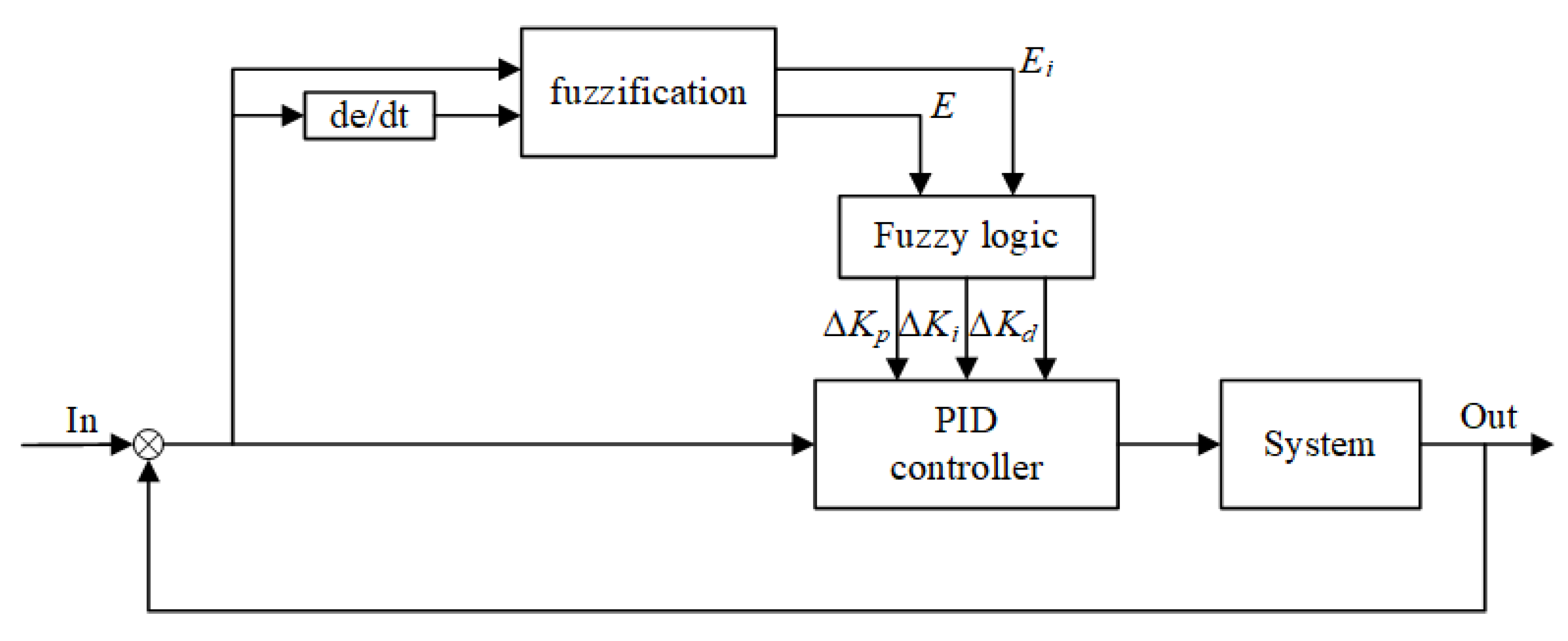
Fuzzy PID (FPID) combines Fuzzy control and PID control, with a simple structure and strong self-adaptability [25]. The fuzzy controller takes error E as the input. The output is the modified values of PID parameters $\Delta K_p$, $\Delta K_i,$ and $\Delta K_d$ through quantization factors, fuzzy control rules, and scale factors. $K_e$ and $K_{ec}$ are quantization factors; $K_{up}$ is the scale factor for $\Delta K_p$; $K_{ui}$ the scaling factor for $\Delta K_i$; and $K_{ud}$ the scaling factor for $\Delta K_d$. 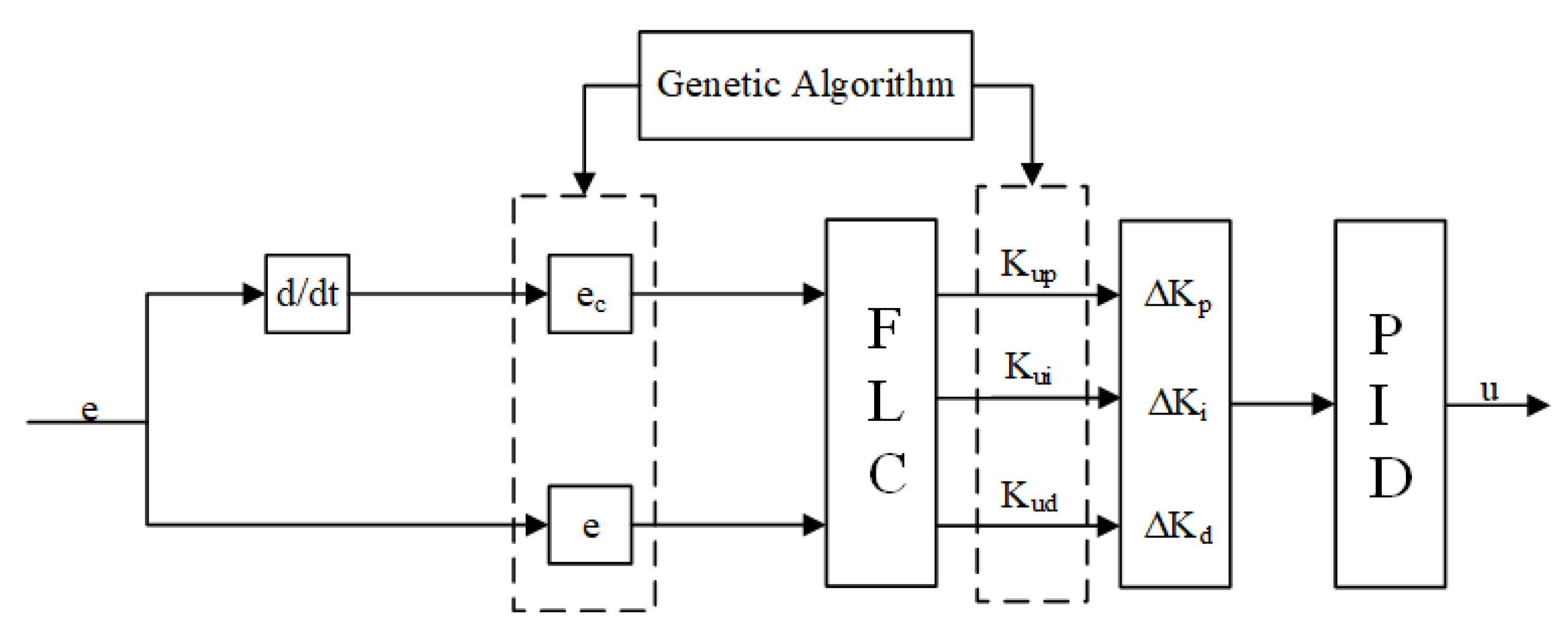Figure 4 shows the block of the fuzzy PID structure. The expression of the fuzzy PID controller is shown in Equation (10).

$$\{\begin{array}{c}{K}_p=K_{p0}+\Delta K_p\\ K_i=K_{i0}+\Delta K_i\\ K_d=K_{d0}+\Delta K_d\end{array}$$

(10)

where $K_{p0}, K_{i0 },$ and $K_{d0}$ represent the proportional, integral, and differential initial coefficients in the traditional PID controller, respectively. Based on the fuzzy rule table, the fuzzy inference results show that $\Delta K_p$,$\Delta K_{i },$ and $\Delta K_{d }$ are the change values of proportion, integral, and differential coefficients, respectively.

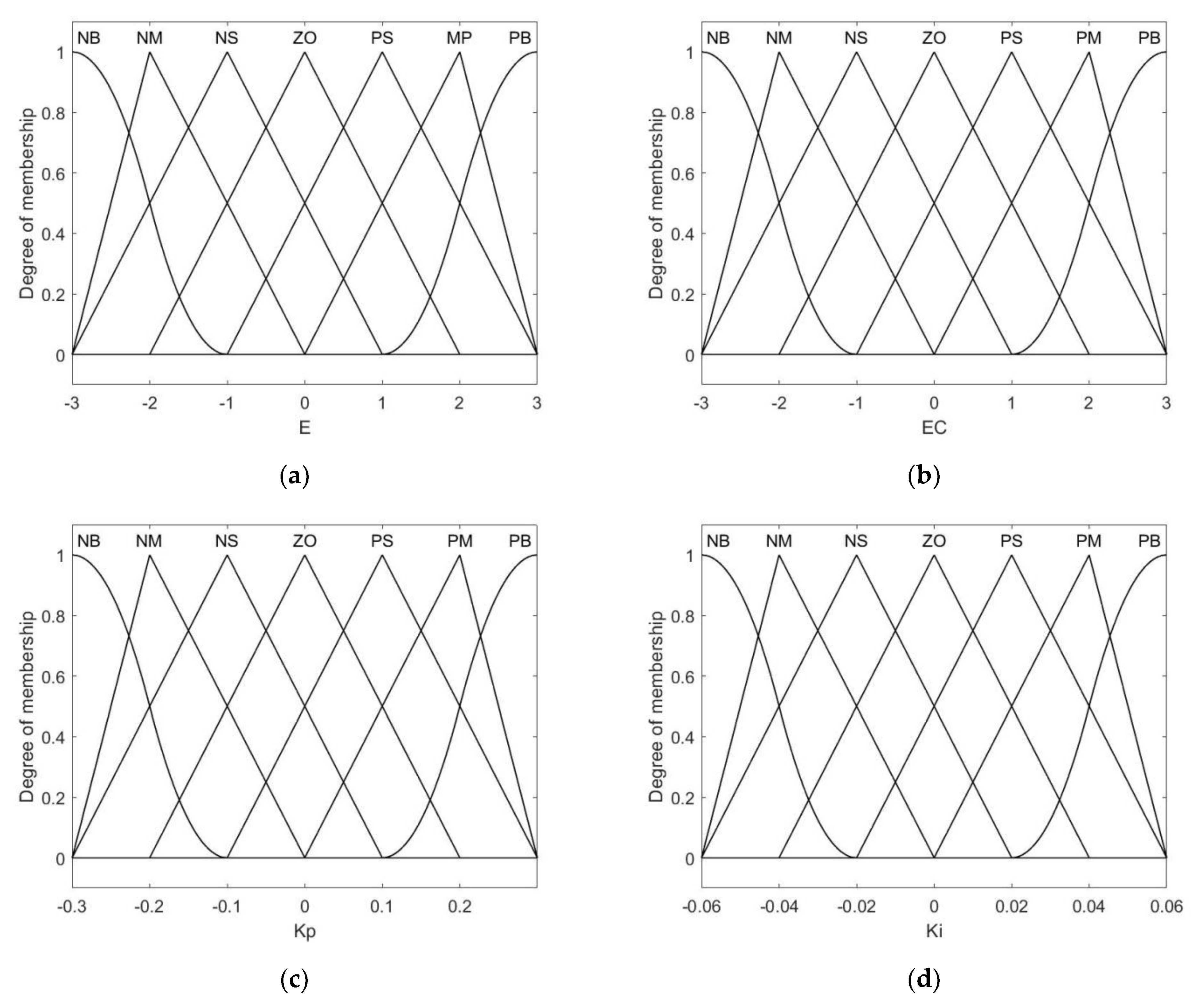
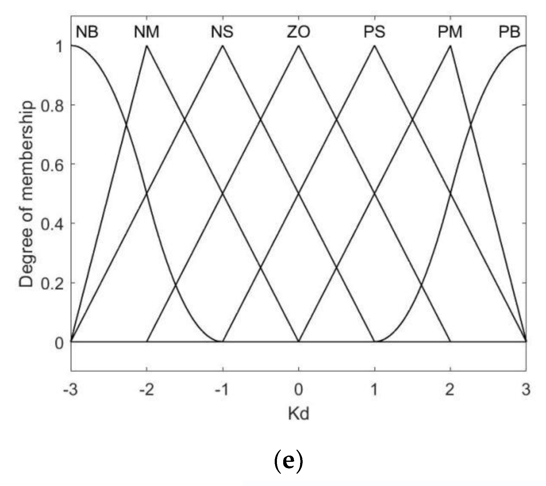
The corresponding membership function is generated by the fuzzy toolbox of mathematical software. Correctly constructing the membership function is one of the keys to using fuzzy control. Figure 5 shows the quantization domain and fuzzy subset. The fuzzy subset with a sharp shape of the membership function has high resolutions and a high control sensitivity. On the contrary, the shape of the membership function curve is relatively flat, with good stability.

The relationship between the three input parameters of the PID controller and the general tuning principles summed up by expert experience are as follows:

(1)

The absolute value of the input error is large. The $K_i$ value is zero; the larger the $K_p$ value, the smaller the $K_d$ value taken simultaneously.

(2)

The absolute value of the input error is the median. $K_i$ takes an appropriate value, and $K_p$ should take a small value. The $K_d$ value significantly affects the system.

(3)

The absolute value of the input error is small. $K_i$ and $K_p$ values should be large, and the $K_d$ value depends on the absolute value of the change rate of the input error. When the change rate is small, $K_d$ takes an intermediate value; otherwise, $K_d$ takes a small value.

Table 1. Fuzzy rule of $\Delta K_p$.

	EC	NB	NM	NS	ZO	PS	PM	PB
E
NB		PB	PB	PM	PM	PS	ZO	ZO
NM		PB	PB	PM	PS	PS	ZO	NS
NS		PM	PM	PM	PS	ZO	NS	NS
ZO		PM	PM	PS	ZO	NS	NM	NM
PS		PS	PS	ZO	NS	NS	NM	NM
PM		PS	ZO	NS	NM	NM	NM	NB
PB		ZO	ZO	NM	NM	NM	NB	NB
NB		PB	PB	PM	PM	PS	ZO	ZO

,

Table 2. Fuzzy rule of $\Delta K_i$.

	EC	NB	NM	NS	ZO	PS	PM	PB
E
NB		NB	NB	NB	NM	NM	NS	ZO
NM		NM	NB	NB	NM	NS	NS	ZO
NS		NS	NB	NM	NS	NS	ZO	PS
ZO		ZO	NM	NM	NS	ZO	PS	PM
PS		PS	NM	NS	ZO	PS	PS	PM
PM		PM	ZO	ZO	PS	PS	PM	PB
PB		PB	ZO	ZO	PS	PM	PM	PB
NB		NB	NB	NB	NM	NM	NS	ZO

and

Table 3. Fuzzy rule of $\Delta K_d$.

	EC	NB	NM	NS	ZO	PS	PM	PB
E
NB		NB	PS	NS	NB	NB	NB	NM
NM		NM	PS	NS	NB	NM	NM	NS
NS		NS	ZO	NS	NM	NM	NS	NS
ZO		ZO	ZO	NS	NS	NS	NS	NS
PS		PS	ZO	ZO	ZO	ZO	ZO	ZO
PM		PM	PB	NS	PS	PS	PS	PS
PB		PB	PB	PM	PM	PM	PS	PS
NB		NB	PS	NS	NB	NB	NB	NM

show fuzzy rules. The input fuzzy variable derivative of position errors has seven linguistic variables, namely NB (negative big), NM (negative medium), NS (negative small), ZO (zero), PS (positive small), PM (positive medium), and PB (positive big). Three points, $\Delta K_p$,$\Delta K_i$, and $\Delta K_d$, are defined as the fuzzy set in the defuzzification process.

4.2. Optimization of Fuzzy PID Parameters by the GA

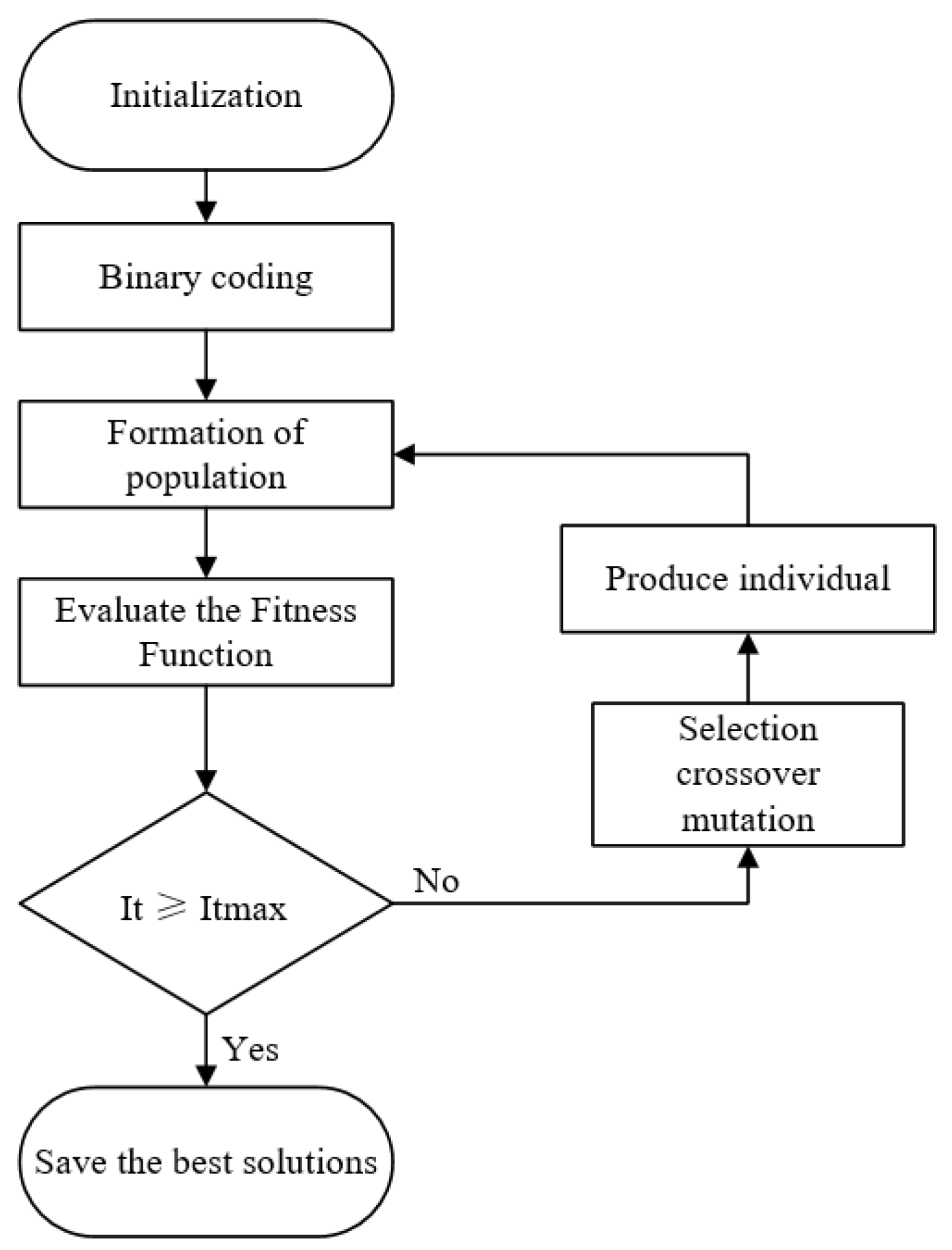
A GA is an optimization method for finding the optimal solution to a problem based on Darwin’s theory of biological evolution [26,27,28]. Traditional fuzzy PID has great differences in selecting rule tables and membership functions, and it is difficult to generalize according to expert experience. The quantization factor and scale factor of the fuzzy PID controller are optimized by the excellent global optimization ability of the GA. The structure diagram of fuzzy PID optimized by genetic algorithm is shown in Figure 6, and the algorithm flow chart is shown in Figure 7:

$\left\{e, e_c, K_p, K_i, K_d\right\}$ are the genes of individuals using the continuous GA to optimize the fuzzy PID controller. Each gene is coded in decimal notation. Fitness function Equation (11) is used to calculate the fitness values of each individual [29]. Equation (12) calculates the probabilities of each individual to be selected [30]:

$$F_i=\frac{1}{{\int }_0^{\infty }\left|e_i\left(t\right)\right|dt}$$

(11)

$$P_i=\frac{F_i}{{\sum }_{i=1}^{n}Fi}$$

(12)

The genetic mode is set to the high probability of crossover and the low probability of mutation and is iterated for 100 generations as the termination condition.

5. Model Building and Simulation Analysis

The Alternating Current (AC) servo motor system is a typical nonlinear controlled object, and it is necessary to comprehensively consider the characteristics of the uncertain system of the AC servo motor. It is assumed that the magnetic circuit is not saturated and the magnetic field is sinusoidal. The eddy current loss and hysteresis loss are ignored. Let $L_d$ = $L_p$ = $L$, and the state Equations (13) and (14) in the d-q coordinates are as follows:

$$G\left(s\right)=\frac{{\mathsf{\omega }}_m\left(\mathrm{s}\right)}{I_m\left(s\right)}=K_{pi}{K}_f{K}_u/JLFF\left(s\right)$$

(13)

$$F\left(s\right)=S^2+\left(R_s+K_{pi}{K}_i\right)S/L+K_f{K}_u/JL$$

(14)

where $K_f, R_s, K_u$, and $K_i$ represent the torque coefficient, stator winding, potential coefficient, and current feedback coefficient, respectively.

Transfer function $G\left(s\right)$ characterizes the dynamic characteristics of the complex system under no moment of inertia and torque interferences. The transfer function is shown in Equation (15):

$$G\left(s\right)=\frac{47.5}{s}-\frac{48}{s+6}+\frac{0.5}{s+534}$$

(15)

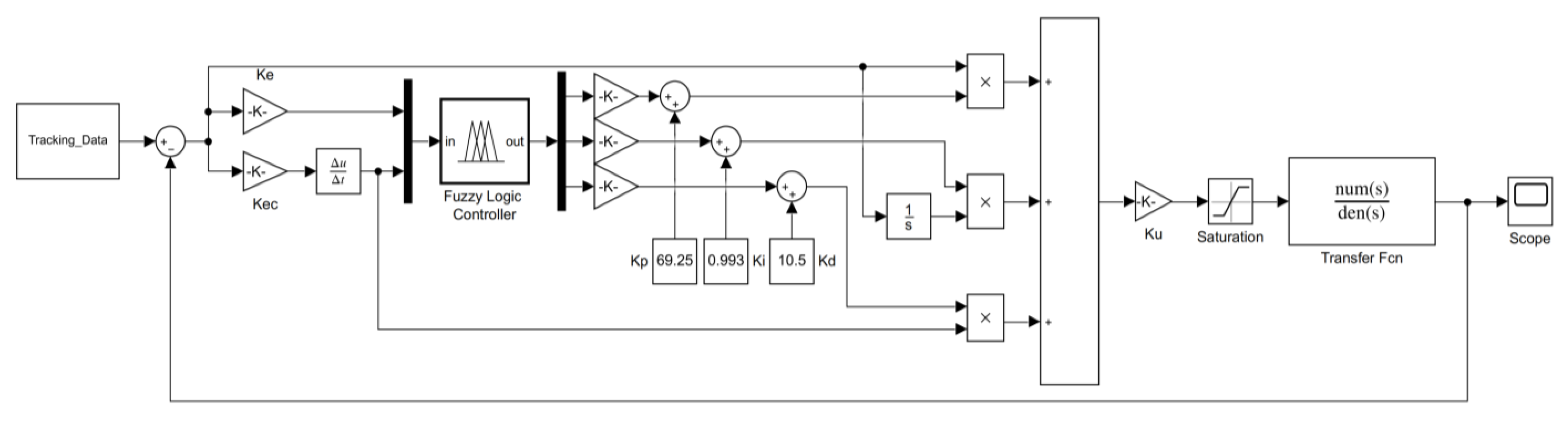
According to the transfer function of the AC servo motor and parameters obtained by the GA, the simulation model is established in mathematical simulation software. The fuzzy PID control system is taken as an example. According to the influence of PID controller parameters on the control effect, combined with fuzzy controller, a fuzzy PID controller is designed (see Figure 8 for the fuzzy PID control model). The three terms used in the block diagram ($K_p$, $K_i$, and $K_d$) are gains for the proportional controller, integral controller, and derivative controller. The values of $K_p$, $K_{i }$, and $K_d$ were 69.25, 0.993, and 10.5, respectively. The values of $K_e$, $K_{ec}$, and $K_u$ were 3, 0. 1, and 0. 1, respectively. The controller dynamically adjusts PID parameters through the GA during the system operation.

6. Analysis of Simulation Results

According to the determined structure and control method of the servo control system, a simulation experiment was carried out on the position control of the servo motor combined with the engineering tuning method. The superiority of the control strategy designed in the work was verified by comparing the control effect of the fuzzy PID (FPID) control strategy and genetic algorithm optimized fuzzy PID (GAFPID) control strategy on the position signal tracking of the servo control system.

6.1. Iterative Analysis of GAs

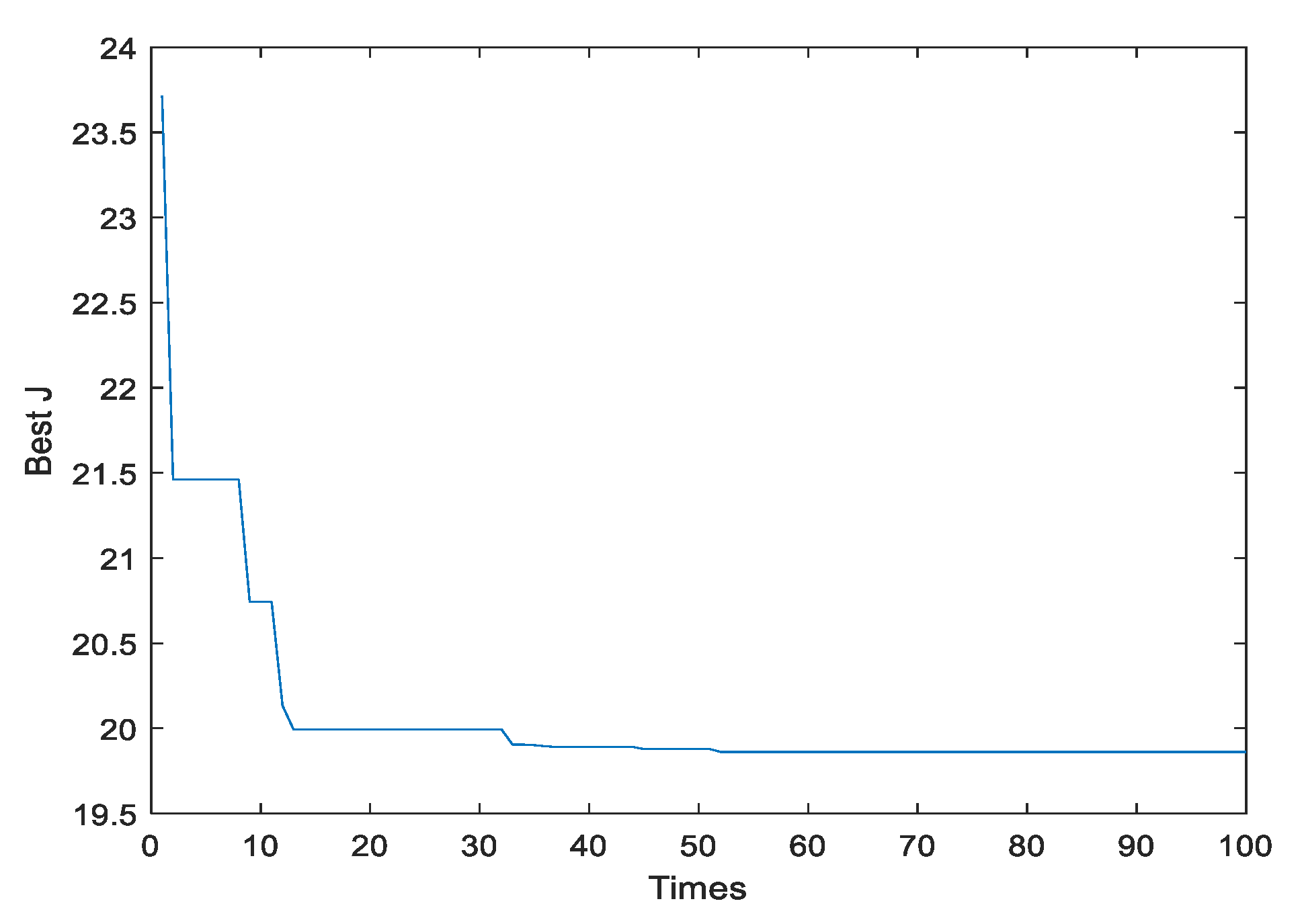
According to the parameters of the setting algorithm of the fuzzy PID control system structure, the population size and the iteration number were set to 30 and 100, respectively. The crossover probability and mutation probability were 0.9 and 0.1, respectively. $K_p=100$, $K_i=100$, and $K_d=10$ at the initial stage.

Figure 9 shows that it converged at the 52nd iteration, while traditional calculations often require thousands of iterations. The traditional method of calculation mentioned here is trial and error. Trial and error is a method of setting parameters empirically. In the closed-loop control system, the adjustment was carried out in the order of $K_p$, $K_i$ and $K_d$. While adjusting the parameters, the process was observed until the requirements were met. The optimal objective function value and the optimal matching parameter value of the fuzzy PID controller could be obtained at the end of the iteration. The parameter values of the fuzzy PID controller obtained by the GA were substituted into the simulation model of the servo control system. The experimental analysis of step characteristics, sinusoidal characteristics, and joint trajectory tracking was carried out.

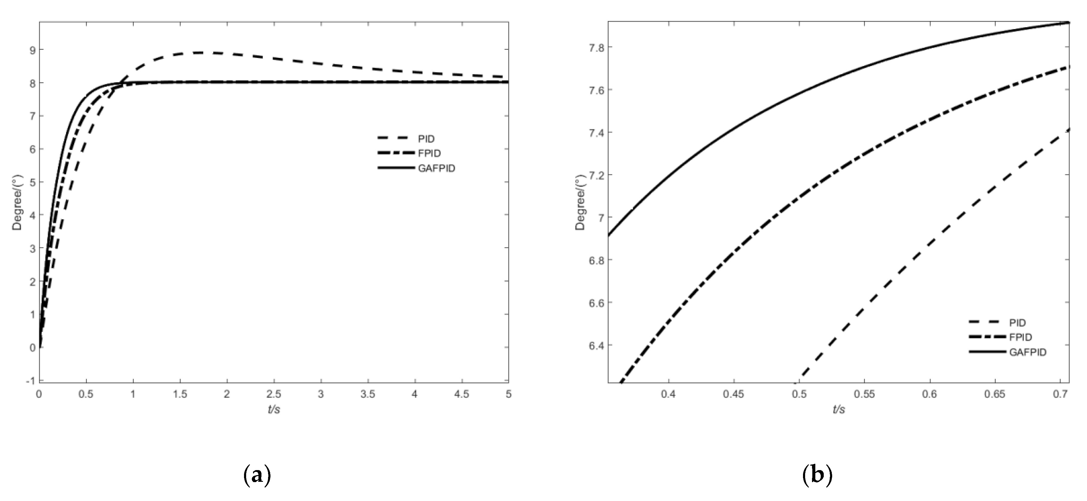
6.2. Simulation Analysis of Step Characteristics

PID control, fuzzy PID control, and PID control optimized by the GA were applied to the control system under the condition that the input was an 8° step signal simulating the load. The sampling time was set to 0.01 s. The dynamic and static indices of the system under different control strategies were analyzed (see Figure 10 for simulation results).

Table 4. Simulation results of the step response.

The Controller Type	Setting Time/(s)	Rise Time/(s)	Steady-State Error/(°)
PID	0.752	0.612	0.1713
FPID	0.654	0.496	0.0209
GAFPID	0.508	0.380	0.0194

shows the simulation results of the step response. The rise time of the system under the control of a fuzzy PID controller optimized by the GA was reduced by about 37.91% compared with the classical PID control under the loaded step response. It was about 23.39% shorter than the fuzzy PID control. The adjustment time of the system controlled by the fuzzy PID controller optimized by the GA was about 32.46% shorter than that of the PID control and about 22.32% shorter than that of the fuzzy PID control. The steady-state error of the system under genetic fuzzy PID control was 88.67% less than that of the classical PID control, and 7.18% less than that of the fuzzy PID control in the steady-state response.

6.3. Sinusoidal Characteristic Simulation Analysis

The input was a 12° sinusoidal signal at 2 Hz to simulate the on-load condition. Four different control strategies were applied to the control system. The sampling time was set to 0.01 s. The maximum amplitude error and the maximum phase error of the system under different control strategies were compared. Figure 11 shows the simulation results.

Table 5. Simulation data of the frequency response under loading.

The Controller Type	Maximum Phase Error/(°)	Maximum Magnitude Error/(°)
PID	0.573	0.2614
FUZZY	1.146	0.6527
FPID	0.344	0.1263
GAFPID	0.229	0.0855

shows the simulation data of frequency response under loading. The sinusoidal signal at 2 Hz and 12° was input under loading. The system under the genetic fuzzy PID control was 32.30% less than the fuzzy PID control system, 80.01% less than the pure fuzzy control system, and 60.03% less than the classical PID control system in terms of the maximum amplitude error. The system under the fuzzy PID control optimized by the GA was 33.43% less than the fuzzy PID, 86.90% less than the pure fuzzy control system, and 67.29% less than the classical PID in terms of the maximum phase error.

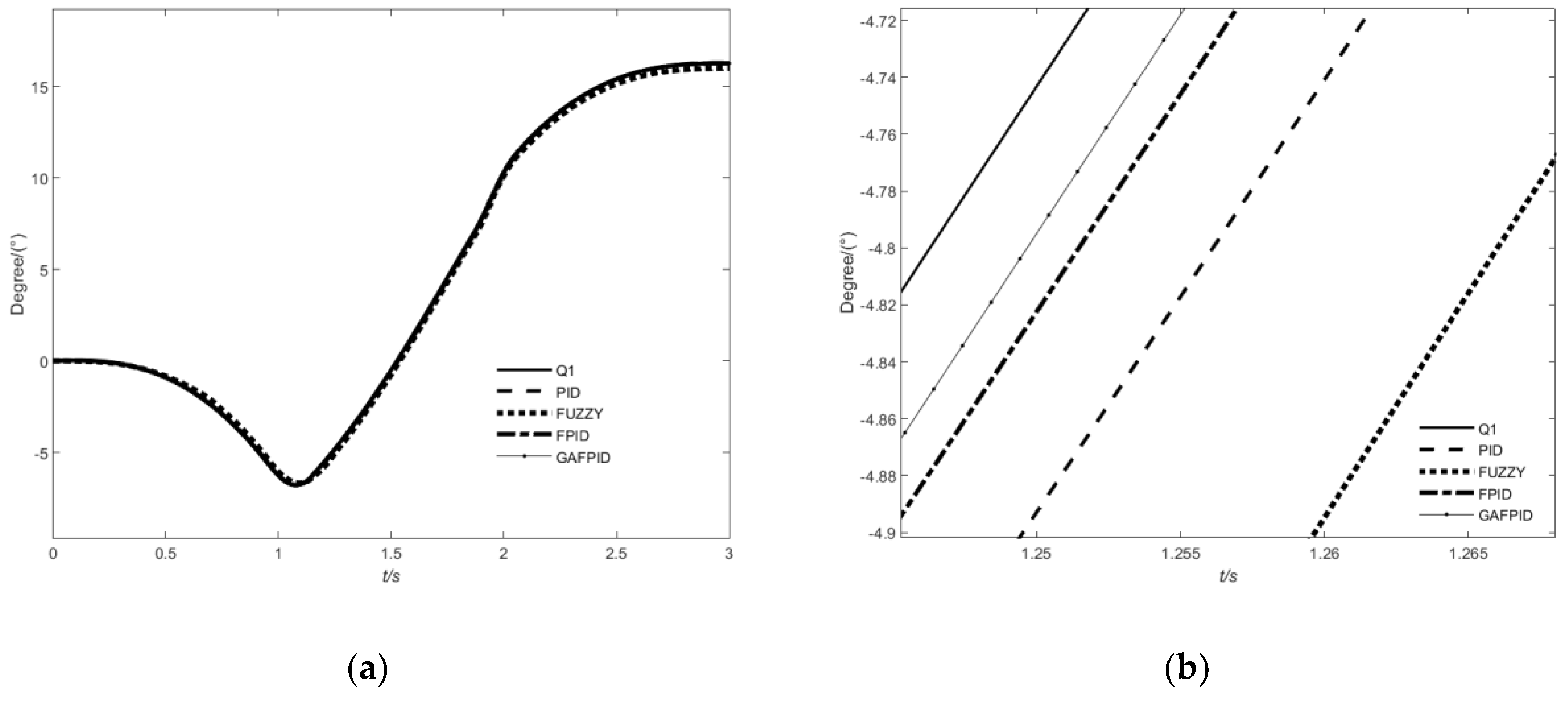
6.4. Input-Joint-Trajectory Simulation Analysis

The controllers of the three joints were successively optimized, and the trajectory planning was carried out in a Cartesian coordinate system. The end effector was moved along the gate-shaped trajectory, and the inverse kinematics were used to map the operation space to the joint space. The trajectories planned by interpolating quintic polynomials were used as the input. The simulation time was set to 3 s. The traditional PID control, fuzzy control, fuzzy PID control, and fuzzy PID control strategies optimized by GAs were used to control the PM. The trajectory tracking capabilities of the four control methods were compared.

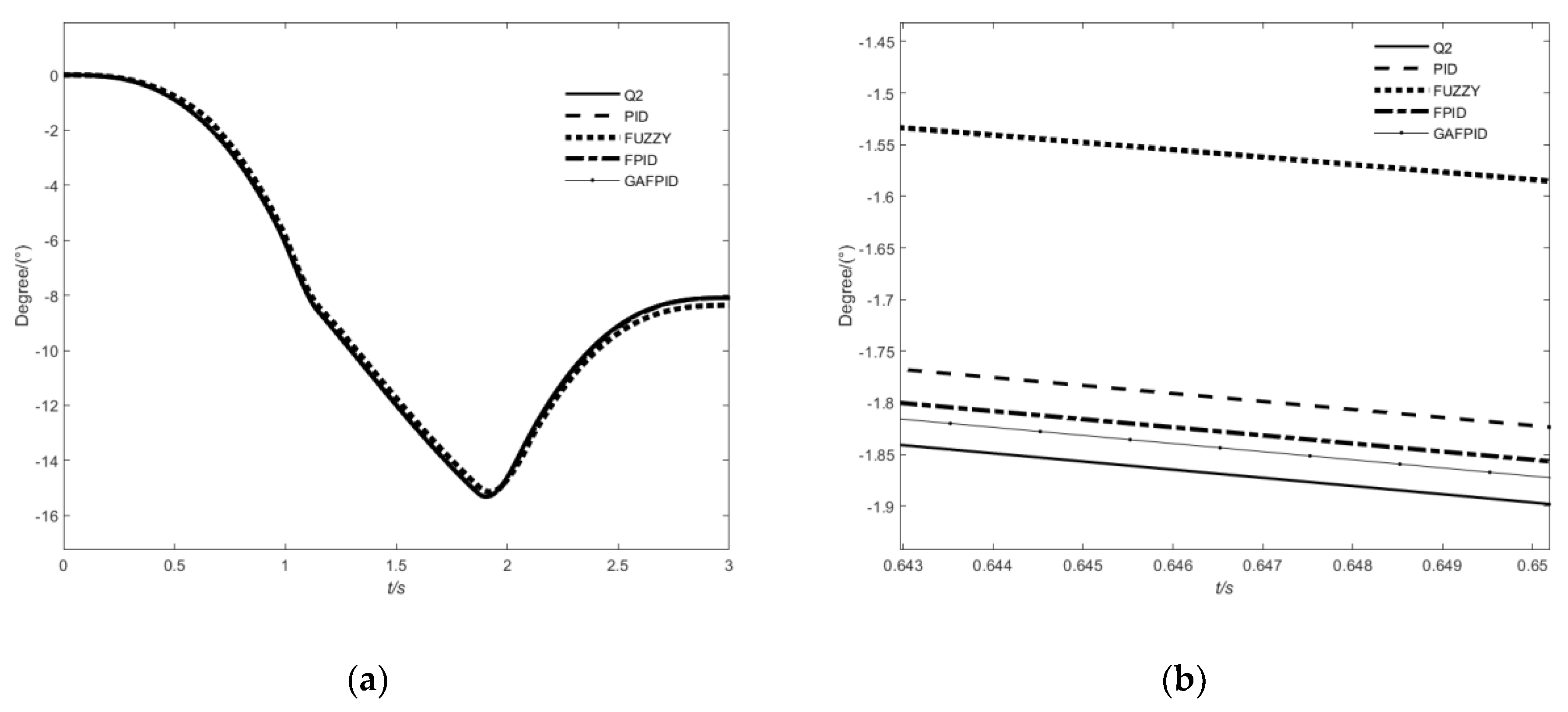
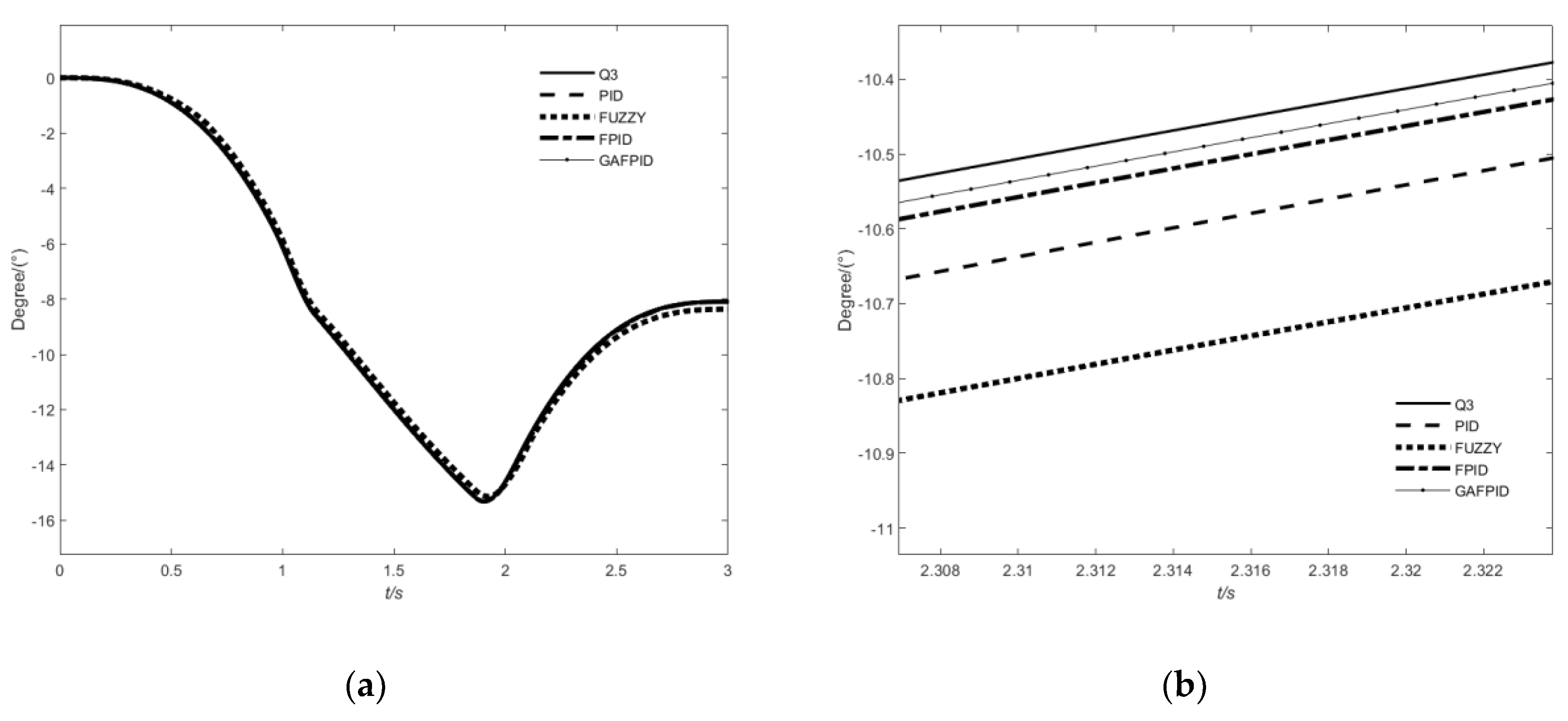
Figure 12, Figure 13 and Figure 14 show the trajectory tracking of the three joints, respectively. The average absolute error was about 0.0327 using the GAFPID control strategy for Q1 joint motion. The enlarged partial image presents that the joint trajectory based on the GAFPID control strategy was the closest to the ideal trajectory, with the optimal control effect.

According to

Table 6. ITAE values.

The Controller Type	Joint Q1	Joint Q2	Joint Q3
PID	0.0655	0.057	0.057
FUZZY	0.1568	0.1667	0.1667
FPID	0.0388	0.0319	0.0319
GAFPID	0.0265	0.0197	0.0197

and

Table 7. IAE values.

The Controller Type	Joint Q1	Joint Q2	Joint Q3
PID	0.0436	0.042	0.042
FUZZY	0.1094	0.1196	0.1196
FPID	0.0237	0.0235	0.0235
GAFPID	0.0147	0.0144	0.0144

, the minimum integral time absolute error (ITAE) value of the joint trajectory is based on the GAFPID control strategy. The dynamic response overshoot was small and the adjustment time was short. The integral absolute error (IAE) index was the smallest, which means that small deviations in the control system can be suppressed.

7. Conclusions

(1)

The PM is a highly nonlinear, strongly coupled, and time-varying control system. It is difficult to obtain the ideal control effect with the traditional control method. In the trajectory tracking control of 3-DOF PM, the PID control was combined to improve the control accuracy. Without relying on the exact mathematical model of the controlled object, the fuzzy control method was used to approximate the nonlinear system. Through the combination of the fuzzy controller and PID controller, a fuzzy PID controller was designed, which could self-tune PID parameters online in the control process. In view of the problem that the design of the fuzzy control system needs expert knowledge and experience to obtain the best control effect, the fuzzy PID controller was optimized by a genetic algorithm.

(2)

The traditional PID control, fuzzy control, fuzzy PID control, and fuzzy PID control optimized by the GA were carried out to simulate signal-tracking and to verify the effectiveness of the optimized controller. The simulation showed that the servo system under the fuzzy PID control based on the GA had significantly improved dynamic response characteristics and steady-state accuracy, with a better trajectory-tracking effect. The ideal control performance of the PM in trajectory tracking control depended on the design of the control system. Through the reasonable selection and design of the control strategy, the control deviation of the joint angle and angular velocity of the PM could be reduced. Thus, the response speed and stability of the system were improved, which is of great significance to the application of PM.

(3)

The optimization of other intelligent algorithms and the combination of each other’s advantages will be further considered in the future to greatly adapt to more complex regulatory processes. The neural network fuzzy control was considered. Neural networks can adequately approximate arbitrary complex nonlinear relationships. It can learn and adapt to the dynamic characteristics of uncertain systems. The adaptive fuzzy control system was introduced, which can identify system parameters and adjust control parameters online. The expert intelligent self-tuning PID controller was used to recognize the system error pattern when the closed-loop system was disturbed. The key problems to be solved in the above control strategy were online parameter identification, parameter adaptive adjustment, the establishment of an expert system, and the combination of a neural network and fuzzy control. The above needs to be studied in further research work.

References

1. Kong, X.; Gosselin, C.M.; Richard, P.-L. Type synthesis of parallel mechanisms with multiple operation modes. In Proceedings of the International Design Engineering Technical Conferences and Computers and Information in Engineering Conference, Philadelphia, PA, USA, 10–13 September 2006; pp. 1037–1046. [Google Scholar] [CrossRef]
2. Huang, Y.; Lu, Q.; Wang, H.; Liu, J.; Li, Z.; Zou, X.; Zhan, X. Kinematics Analysis and Simulation of a Novel 3T Parallel Mechanism. Math. Probl. Eng. 2022, 2022, 3424012. [Google Scholar] [CrossRef]
3. Ziegler, J.G.; Nichols, N.B. Optimum settings for automatic controllers. Trans. ASME 1942, 64, 759–768. [Google Scholar] [CrossRef] [Green Version]
4. Li, H.-X.; Gatland, H. A new methodology for designing a fuzzy logic controller. IEEE Trans. Syst. Man Cybern. 1995, 25, 505–512. [Google Scholar] [CrossRef]
5. Carvajal, J.; Chen, G.; Ogmen, H. Fuzzy PID controller: Design, performance evaluation, and stability analysis. Inf. Sci. 2000, 123, 249–270. [Google Scholar] [CrossRef]
6. Najafizadeh Sari, N.; Jahanshahi, H.; Fakoor, M. Adaptive fuzzy PID control strategy for spacecraft attitude control. Int. J. Fuzzy Syst. 2019, 21, 769–781. [Google Scholar] [CrossRef]
7. Zhou, H.; Chen, R.; Zhou, S.; Liu, Z. Design and analysis of a drive system for a series manipulator based on orthogonal-fuzzy PID control. Electronics 2019, 8, 1051. [Google Scholar] [CrossRef] [Green Version]
8. Phu, N.D.; Hung, N.N.; Ahmadian, A.; Senu, N. A new fuzzy PID control system based on fuzzy PID controller and fuzzy control process. Int. J. Fuzzy Syst. 2020, 22, 2163–2187. [Google Scholar] [CrossRef]
9. Phu, N.D.; Hung, N.N. Some solving methods for a fuzzy multi-point boundary value problem. Soft Comput. 2020, 24, 483–499. [Google Scholar] [CrossRef]
10. Liu, Y.; Fan, K.; Ouyang, Q. Intelligent traction control method based on model predictive fuzzy PID control and online optimization for permanent magnetic maglev trains. IEEE Access 2021, 9, 29032–29046. [Google Scholar] [CrossRef]
11. Tsai, C.-C.; Yu, C.-C.; Tsai, C.-T. Adaptive ORFWNN-based predictive PID control. Int. J. Fuzzy Syst. 2019, 21, 1544–1559. [Google Scholar] [CrossRef]
12. Pelusi, D. Optimization of a fuzzy logic controller using genetic algorithms. In Proceedings of the 2011 Third International Conference on Intelligent Human-Machine Systems and Cybernetics, Hangzhou, China, 26–27 August 2011; pp. 143–146. [Google Scholar] [CrossRef]
13. Pelusi, D. Designing neural networks to improve timing performances of intelligent controllers. J. Discret. Math. Sci. Cryptogr. 2013, 16, 187–193. [Google Scholar] [CrossRef]
14. Pelusi, D.; Mascella, R. Optimal control Algorithms for second order Systems. J. Comput. Sci. 2013, 9, 183–197. [Google Scholar] [CrossRef] [Green Version]
15. Purnama, H.S.; Sutikno, T.; Alavandar, S.; Subrata, A.C. Intelligent control strategies for tuning PID of speed control of DC motor: A review. In Proceedings of the 2019 IEEE Conference on Energy Conversion (CENCON), Yogyakarta, Indonesia, 16–17 October 2019; pp. 24–30. [Google Scholar] [CrossRef]
16. Singh, A.; Giri, V. Design and analysis of DC motor speed control by GA based tuning of fuzzy logic controller. Int. J. Eng. Res. Technol. 2012, 1, 1–6. [Google Scholar]
17. Chao, C.-T.; Sutarna, N.; Chiou, J.-S.; Wang, C.-J. An optimal fuzzy PID controller design based on conventional PID control and nonlinear factors. Appl. Sci. 2019, 9, 1224. [Google Scholar] [CrossRef] [Green Version]
18. Chao, C.-T.; Sutarna, N.; Chiou, J.-S.; Wang, C.-J. Equivalence between fuzzy PID controllers and conventional PID controllers. Appl. Sci. 2017, 7, 513. [Google Scholar] [CrossRef] [Green Version]
19. Flores-Morán, E.; Yánez-Pazmiño, W.; Barzola-Monteses, J. Genetic algorithm and fuzzy self-tuning PID for DC motor position controllers. In Proceedings of the 2018 19th International Carpathian Control Conference (ICCC), Szilvasvarad, Hungary, 28–31 May 2018; pp. 162–168. [Google Scholar] [CrossRef]
20. Morán, M.E.F.; Viera, N.A.P. Comparative study for DC motor position controllers. In Proceedings of the 2017 IEEE Second Ecuador Technical Chapters Meeting (ETCM), Salinas, Ecuador, 16–20 October 2017; pp. 1–6. [Google Scholar] [CrossRef]
21. Vijaya, S.; Bharathiraja, P.; Nithyanandam, J. A Performance Comparison of Conventional and New Seven Level Inverter Topology Fed PM Synchronous Motor Using GA Based Fuzzy PID Speed Controller. In Proceedings of the 2018 International Conference on Computation of Power, Energy, Information and Communication (ICCPEIC), Chennai, India, 28–29 March 2018; pp. 275–279. [Google Scholar] [CrossRef]
22. Dogruer, T.; Can, M.S. Design and robustness analysis of fuzzy PID controller for automatic voltage regulator system using genetic algorithm. Trans. Inst. Meas. Control 2022, 44, 1862–1873. [Google Scholar] [CrossRef]
23. Alouache, A.; Wu, Q. Genetic algorithms for trajectory tracking of mobile robot based on PID controller. In Proceedings of the 2018 IEEE 14th International Conference on Intelligent Computer Communication and Processing (ICCP), Cluj-Napoca, Romania, 6–8 September 2018; pp. 237–241. [Google Scholar] [CrossRef]
24. Ang, K.H.; Chong, G.; Li, Y. PID control system analysis, design, and technology. IEEE Trans. Control Syst. Technol. 2005, 13, 559–576. [Google Scholar] [CrossRef] [Green Version]
25. Tang, K.-S.; Man, K.F.; Chen, G.; Kwong, S. An optimal fuzzy PID controller. IEEE Trans. Ind. Electron. 2001, 48, 757–765. [Google Scholar] [CrossRef] [Green Version]
26. Forrest, S. Genetic algorithms. ACM Comput. Surv. 1996, 28, 77–80. [Google Scholar] [CrossRef]
27. Holland, J.H. Genetic algorithms. Sci. Am. 1992, 267, 66–73. [Google Scholar] [CrossRef]
28. Sivanandam, S.; Deepa, S. Genetic algorithms. In Introduction to Genetic Algorithms; Springer: Berlin/Heidelberg, Germany, 2008; pp. 15–37. [Google Scholar] [CrossRef]
29. Mahfud, S.; Derouich, A.; El Ouanjli, N.; Mossa, M.A.; Motahhir, S.; El Mahfoud, M.; Al-Sumaiti, A.S. Comparative Study between Cost Functions of Genetic Algorithm Used in Direct Torque Control of a Doubly Fed Induction Motor. Appl. Sci. 2022, 12, 8717. [Google Scholar] [CrossRef]
30. Lin, C.-L.; Jan, H.-Y.; Shieh, N.-C. GA-based multiobjective PID control for a linear brushless DC motor. IEEE/ASME Trans. Mechatron. 2003, 8, 56–65. [Google Scholar] [CrossRef]
Figure 1. PM structure.
Applsci 12 11128 g001
Figure 2. Established coordinate system.
Applsci 12 11128 g002
Figure 3. Door-shaped trajectory.
Applsci 12 11128 g003
Figure 4. Fuzzy PID controller.
Applsci 12 11128 g004
Figure 5. Membership function: (a) error; (b) changes in errors; (ce) K p , K i , and K d membership functions for fuzzy self-tuning PID, respectively.
Applsci 12 11128 g005aApplsci 12 11128 g005b
Figure 6. Structure of the GA to optimize fuzzy PID.
Applsci 12 11128 g006
Figure 7. Flow of the GA.
Applsci 12 11128 g007
Figure 8. Blocks of the fuzzy self-tuning PID control algorithm.
Applsci 12 11128 g008
Figure 9. Iterative curve of the GA.
Applsci 12 11128 g009
Figure 10. (a) Step response; (b) local enlarged view.
Applsci 12 11128 g010
Figure 11. Sinusoidal input signal at 2 Hz: (a) tracking response; (b) local enlarged view.
Applsci 12 11128 g011
Figure 12. Joint trajectory Q1: (a) tracking response; (b) local enlarged view.
Applsci 12 11128 g012
Figure 13. Joint trajectory Q2: (a) tracking response; (b) local enlarged view.
Applsci 12 11128 g013
Figure 14. Joint trajectory Q3: (a) tracking response; (b) local enlarged view.
Applsci 12 11128 g014