An Adaptive Dynamic Channel Allocation Algorithm Based on a Temporal–Spatial Correlation Analysis for LEO Satellite Networks

Abstract

Low Earth orbit (LEO) satellites that can be used as computing nodes are an important part of future communication networks. However, growing user demands, scarce channel resources and unstable satellite–ground links result in the challenge to design an efficient channel allocation algorithm for the LEO satellite network. Edge computing (EC) provides sufficient computing power for LEO satellite networks and makes the application of reinforcement learning possible. In this paper, an adaptive dynamic channel allocation algorithm based on a temporal–spatial correlation analysis for LEO satellite networks is proposed. First, according to the user mobility model, the temporal–spatial correlation of handoff calls is analyzed. Second, the dynamic channel allocation process in the LEO satellite network is formally described as a Markov decision process. Third, according to the temporal–spatial correlation, a policy for different call events is designed and online reinforcement learning is used to solve the channel allocation problem. Finally, the simulation results under different traffic distributions and different traffic intensities show that the proposed algorithm can greatly reduce the rejection probability of the handoff call and then improve the total performance of the LEO satellite network.

1. Introduction

Satellite networks not only provide a call admission service to terminal users at any time and anywhere, but also provide reliable communication in many scenes such as natural disasters and emergency rescues. Therefore, it has become a favorable supplement to terrestrial networks [1]. Low Earth orbit (LEO) satellite networks have advantages such as global coverage, real-time communication and small terminals, which makes them a research hotspot of satellite networks [2]. Several researchers have combined LEO satellite networks with edge computing (EC) to deploy EC servers on LEO satellites [3,4,5]. As edge computing nodes, LEO satellites are an important part of future communication networks [6]. The effectiveness of the application of an EC framework has been verified in existing systems [7,8,9]. A reasonable channel allocation algorithm can improve the utilization of communication resources and the performance of satellite networks. Edge computing provides sufficient computing power for LEO satellites and makes it possible to apply reinforcement learning to channel allocations [10].

LEO satellites operate at a low altitude with a high speed, which makes its coverage area prone to handoff. Therefore, the visibility time of LEO satellites to terminal users is very short. By using multiple antennas and a satellite-fixed cell (SFC) mode, the coverage area is divided into multi-beams. Each beam is called as a cell [11]. A call for the terminal user will hand over between multiple cells or multiple satellites during the whole communication process. Each handoff will cause a reallocation of the channel resources. An efficient channel allocation algorithm can reduce the rejection probability of calls and improve the total performance of LEO satellite networks [12].

In recent years, scholars have researched channel allocation algorithms in LEO satellite networks [13,14,15,16,17,18]. A fixed channel allocation (FCA) algorithm can allocate unchanged channels in each specified cell. Del Re et al. [19] analyzed the performance of an FCA for LEO satellite networks. An FCA is simple to implement, but it has a poor adaptability to variations in the demands of terminal users. A dynamic channel allocation (DCA) algorithm is superior to an FCA in performance. Li et al. [20] used a DCA to improve the resource utilization in a satellite network. However, the computational complexity of a DCA is higher than that of an FCA. Reinforcement learning (RL) is suitable for solving the DCA problem [21]. Nie et al. [22] used Q-learning to solve the DCA problem and reduce the computational complexity. Hu et al. [23] proposed a deep RL framework to solve the DCA problem and further improve the resource utilization in a satellite network. Liu et al. [24] considered the temporal correlation of a satellite network and used deep RL to further improve the resource utilization. Zheng et al. [25] extracted the state features through a convolution neural network and used deep learning to solve the DCA problem. The above scholars optimized a DCA with RL, which effectively improved the resource utilization in LEO satellite networks. However, LEO satellite networks have the problem of frequent handoffs. The existing dynamic channel allocation algorithms based on RL rarely evaluate the performance of handoff calls.

The channel reservation technique is an effective way to resolve the problem of frequent handoffs [26]. Maral et al. [27] designed a channel locking mechanism for handoff users with a successful handoff. Del Re et al. [28] proposed different handoff queueing strategies with dynamic and fixed channel allocation techniques. However, it is difficult to balance the complexity and performance. A channel allocation algorithm combined with RL technology can be implemented more flexibly and efficiently [29,30]. The traffic prediction of the calls of terminal users plays a decisive role in the resource allocation [31]. Due to LEO satellites moving along their orbit regularly and periodically, a handoff call has the characteristic of a temporal–spatial correlation. The temporal correlation means that the departure call of the current cell and the new call of the adjacent cell occur at the same time. The spatial correlation means that the adjacent cell and the current cell have a neighbor relationship in space. We made full use of the temporal–spatial correlation of handoff calls in LEO satellite networks to propose an adaptive DCA algorithm based on RL. This algorithm not only considered the problems caused by a frequent handoff, but also improved the total performance of the network. The main efforts of this paper were:

• The temporal–spatial correlation of handoff calls was analyzed and the Markov decision process (MDP) was used to formally describe the channel allocation process so that the channel allocation could be dynamically adjusted according to the environment.
• A policy for different call events was designed. Afterwards, an online RL algorithm—namely, SARSA—was used to solve the DCA problem. SARSA iteratively updated the policy from the performed actions so that the channel allocation could be adjusted in real-time according to the environment.
• The effectiveness of the proposed algorithm was verified by simulation experiments under different traffic distributions and different traffic intensities.

The remainder of this paper is structured as follows. Section 2 introduces the related technologies. The proposed algorithm is presented in Section 3. Section 4 presents and discusses the simulation results. Finally, conclusions are drawn in Section 5.

2. Related Technologies

2.1. Markov Decision Process

The MDP, which is a discrete time stochastic control process, provides a mathematical framework for modeling the decision process [32,33]. Typically, the MDP is defined as a tuple (S, A, P, R), where S represents a finite set of states and A represents a finite set of actions. P represents the probability of the state transition from s (s∈S) to s’ (s’∈S) after performing an action a (a∈A). R represents the immediate reward obtained after performing this action. In the MDP, policy π is defined as the mapping from a state to an action. The ultimate goal of the MDP is to find the optimal policy π* to maximize the benefit that the performed actions can cumulatively obtain from the environment.

2.2. SARSA

RL, an important branch of machine learning, is an effective way to solve the MDP. The state-action value is very important in RL, which is called the Q-value. The Q-value refers to the average value of the benefits cumulatively obtained from the environment when a policy π performs an action from the current state to the final state. It is generally expressed as the expectation of the sum of the immediate reward and the subsequent rewards. The Q-value is a measure of the quality of the policy and it is calculated by:

$$Q\left(s_t,a_t\right)=E_{\pi }\left(R_t+\gamma R_{t+1}+{\gamma }^2{R}_{t+2}+{\gamma }^3{R}_{t+3}+\dots |s_t=s,a_t=a\right)$$

(1)

where s_t is the environmental state at time t, a_t is the performed action at time t and π is the policy. In particular, R_t is the immediate reward after performing action a_t in the state s_t and R_t+1, R_t+2 … are the subsequent rewards after time t. γ ∈ [0,1) is the discount factor, which weighs the immediate reward and subsequent rewards obtained after performing the current action.

Finding the optimal policy means that an optimal action is performed at each state. When the space of the environmental state is very large or the probability of the current state reaching the final state is very small, it is difficult for Equation (1) to update the Q-value. Q-learning can update the Q-value in one step with the learning rate.

SARSA can calculate the Q-value of a given policy without a state transition probability and complete the state sequence so it can find the optimal policy without requiring knowledge of the environment [34,35]. Different from Q-learning, SARSA performs the actions with the same policy in real-time at each iteration time step [36,37]. Its Q-value is iteratively updated at each time step by:

$$Q_{t+1}\left(s_t,a_t\right)=Q_t\left(s_t,a_t\right)+{\alpha }_t\left[R_t\left(s_t,a_t\right)+\gamma Q_t\left(s_{t+1},a_{t+1}\right)-Q_t\left(s_t,a_t\right)\right]$$

(2)

where ${\alpha }_t$ is the learning rate at time t and $Q_t\left(s_{t+1},a_{t+1}\right)$ is the value of the next state and the next action. According to ${\alpha }_{t+1}={\alpha }_t*$δ, the learning rate decreases with an increase in the iteration time t. δ is the decay factor of α and ${\alpha }_t$∈ (0,1].

3. The Proposed Algorithm

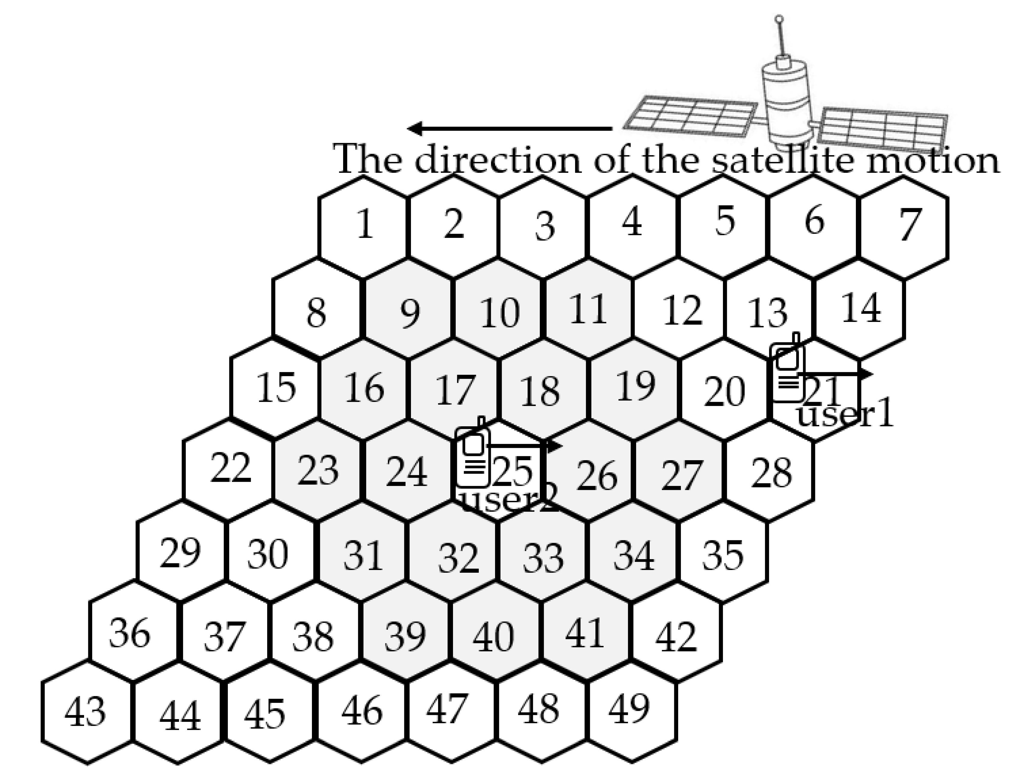
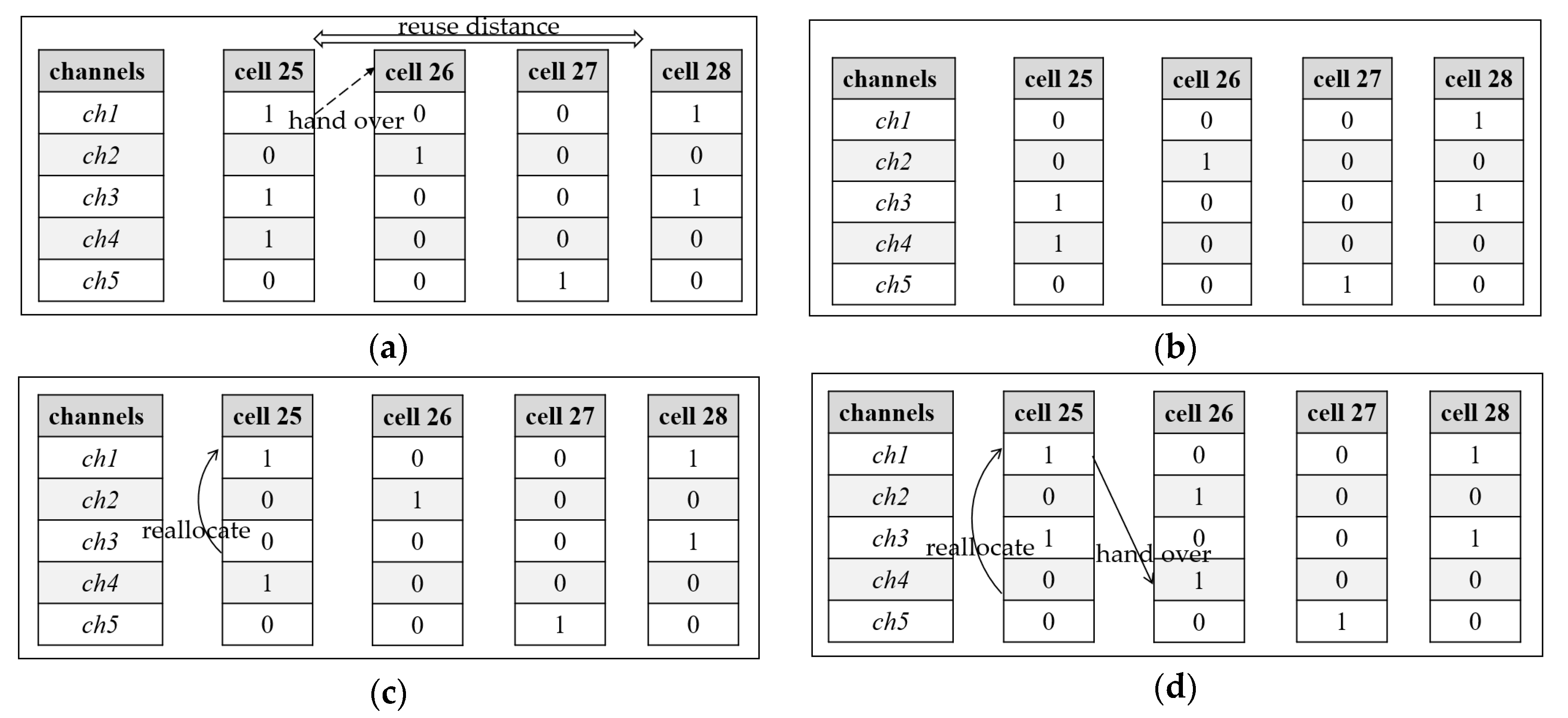
3.1. Temporal–Spatial Correlation Analysis

The mobility model of the users is shown in Figure 1. The LEO satellite used the SFC coverage mode. The user mobility was simplified to a linear motion. Compared with the satellite movement speed, the speed of the terminal users had the same value and the opposite direction [38].

The high-speed movement of LEO satellites makes calls frequently hand over between cells or satellites. The departure call of the current cell and the new call of the adjacent cell occur at the same time. A handoff call occurs in the only neighbor cell that is in the opposite direction to the satellite movement. Therefore, a handoff call has the characteristic of a temporal–spatial correlation in LEO satellite networks.

A call of the current cell hands over at a certain time because of the high-speed movement of the LEO satellite. The call of the current cell departs; meanwhile, a new call of the adjacent cell occurs. The adjacent cell is the only neighbor cell where the call of the current cell hands over. As shown in Figure 1, cell 19 is the adjacent cell of cell 18. In other words, the call of cell 18 will hand over to cell 19.

When a handoff call occurs, the channel allocation algorithm not only releases the occupied channel for the departure call, but also allocates the channel for the handoff call of the adjacent cell. Generally speaking, one channel resource is usually allocated for one call in LEO satellite networks. The allocated channel must also meet any electromagnetic compatibility constraints to avoid co-channel interference [39].

We assumed that the LEO satellite network had N cells Շ = {1, 2, 3, …… N} and K channels Ҡ = {1, 2, 3, …… K}. The conflicting cell I(n) of cell n referred to the cells whose distances from themselves to cell n were less than the minimal reuse distance. This could be expressed by:

I(n) = {m∈Շ, dist(n, m) < d}

(3)

where dist(n, m) represents the distance between cell n and cell m and d represents the minimal reuse distance. As shown in Figure 1, the 18 cells in gray were conflicting the cell of cell 25 if d = 3.

The same channel cannot simultaneously be allocated to the calls of the current cell and its conflicting cell. The eligible channel Ã(n) of cell n refers to the idle channel in both cell n itself and its conflicting cell and can be expressed by:

Ã(n) = {k∈Ҡ, ∑_m∈I(n) x(m, k) = 0}

(4)

where x(m, k) represents the status of channel k of cell m. The value 0 means idle and 1 means occupied.

3.2. Markov Decision Process for the Dynamic Channel Allocation Process

In this paper, the channel status and the call event formed the environment in the channel allocation problem. The transition of the environmental state had the Markov property. The whole channel allocation process was described as per the following MDP model to dynamically adapt to the environmental changes.

State S: s_t = (X_t, e_t) represents the environmental state at time t. X_t is the channel status of the LEO satellite network at time t and e_t is the call event for the admission service to the terminal users at time t. They are expressed, respectively, by:

$$X_t=\left[\begin{array}{ccccccc}{x}_t\left(1, 1\right)& x_t\left(1, 2\right)& x_t\left(1, 3\right)& \dots & x_t\left(1, k\right)& \dots & x_t\left(1,K\right)\\ x_t\left(2, 1\right)& x_t\left(2, 2\right)& x_t\left(2,,, ,3\right)& \dots & x_t\left(2, k\right)& \dots & x_t\left(2,K\right)\\ \dots & \dots & \dots & \dots & \dots & \dots & \dots \\ x_t\left(n, 1\right)& x_t\left(n, 2\right)& x_t\left(n,3\right)& \dots & x_t\left(n, k\right)& \dots & x_t\left(n,K\right)\\ x_t\left(N,1\right)& x_t\left(N,2\right)& x_t\left(N,3\right)& \dots & x_t\left(N, k\right)& \dots & x_t\left(N,K\right)\end{array}\right]$$

(5)

$$e_t \in \{e_{n,t}^{new}, e_{n,m,k,t}^{handoff}, e_{n,k,t }^{end}\}$$

(6)

where x_t(n, k) = 0 represents that channel k of cell n is idle at time t and x_t(n, k) = 1 represents that this channel is occupied. $e_{n,t}^{new}$ represents a new call event in cell n at time t. $e_{n,m,k,t}^{handoff}$represents that the handoff call event on channel k in cell n will hand over to the adjacent cell m at time t according to its temporal–spatial correlation. $e_{n,k,t}^{end}$ represents that the departure call event on channel k in cell n occurs at time t.

Action A: to accept or reject the call event. If a new call arrives, a channel should be occupied. If the call departs, a channel should be free. If the call hands over, the related new call and the departure call should be handled. In this paper, the actions of different call events were expressed by:

$$A\left(\left(x_t,e_t\right)\right)=\left\{\begin{array}{c}Ã\left(n\right), e_t=e_{n,t}^{new}\\ \left\{l\in \mathrm{K},x_t\left(n,l\right)=1\right\}, e_t=e_{n,k,t}^{end}\\ A\left(\left(x_t,e_{n,k,t}^{end}\right)\right)\cup A\left(\left(x_{t+1},e_{m,t}^{new}\right)\right) e_t=e_{n,m,k,t}^{handoff}\end{array}\right.$$

(7)

Immediate reward R: the reward obtained from the environment after performing action a_t in the current state s_t. In this paper, the immediate reward referred to the total number of calls served in the current network. It was expressed by:

$$R_t=(s_t, ) {{\displaystyle \sum }}_{n=1}^N{{\displaystyle \sum }}_{k=1}^K{x}_{t+1 }(n, k)$$

(8)

where x_t+1(n, k) represents the transformed status of channel k in cell n after performing action a_t.

Policy π: the mapping from an environmental state to the performed action. The performed action in the current state corresponds with the selected channel for the current call. The relationship between action, state and policy is expressed by:

a_t = π(s_t = (X_t, e_t))

(9)

3.3. SARSA for Solving the MDP Model

RL can discover an optimal policy and obtain the maximal benefit from the environment. As an online RL algorithm, SARSA was used in this paper to solve the MDP for the channel allocation process. SARSA selected the optimal actions at each time step in real-time and directly updated the policy by the performed actions through interacting with the environment so that the channel allocation algorithm could be adjusted in real-time with the environmental changes.

First, parameters such as the channel status, the Q-value, the learning rate and the discount factor were initialized. Second, by using the temporal–spatial correlation of handoff calls, action a_t was performed according to the policy π for different call events. Subsequently, the immediate reward R_t was obtained after performing a_t and then the environment reached a new state. Third, with the same policy, an action was selected for the next call event and the current Q-value was updated. Last, the iteration continued in the new state until the ending conditions were satisfied. SARSA for solving the MDP model is shown in Algorithm 1.

Algorithm 1: SARSA for solving the MDP model

Input: α, δ, γ Output: Q*(s, a)X ←x0(n, k) = 0 ⧠⧠ //initialize the channel statusQ(s, a) = 0 //initialize the Q-value while list { call event } ≠ Ф do ⧠⧠⧠⧠ if et ==$e_{n,t}^{new}$ at ←$\pi \left(s_t=\left(X_t,e_{n,t}^{new}\right)\right)$ //perform at for the new call event else if et == $e_{n,k,t}^{end}$ at ← $\pi \left(s_t=\left(X_t,e_{n,k,t}^{end}\right)\right)$ //perform at for the departure call event else if et ==$e_{n,m,k,t}^{handoff}$ at ← $\pi \left(s_t=\left(X_t,e_{n,m,k,t}^{handoff}\right)\right)$ //perform at for the handoff call event end if Xt+1 ← z(st, at) //transform the channel status $R_t={\sum }_{n=1}^N{\sum }_{k=1}^K{x}_{t+1}\left(n,k\right)$ //calculate the immediate reward Update Q(st, a) α ← α * δ //decline the learning rate with the decay factor δ st ← st+1 t = t + 1

end

In view of different call events, the proposed algorithm had the following policy. For a new call event and a departure call event, the actions were performed with ε-greedy and then the Q-value was updated. For a handoff call event, two actions were successively performed with the temporal–spatial correlation of the handoff calls and then the Q-value was updated. The policy is described in detail below.

3.3.1. The New Call Event

When a new call event occurred (e_t =$e_{n,t}^{new}$), the current state was s_t = (X_t, $e_{n,t}^{new}$). If the eligible channel Ã(n) was empty, the new call was rejected. Otherwise, the channel was allocated for the new call in the current state. The policy for the new call event was expressed by:

$$\mathsf{\pi }(s=(X_t, e_{n,t}^{new}\left)\right) \left\{\begin{array}{c}random Ã\left(n\right), \epsilon \\ arg max Q\left(s_t,a\right), 1-\epsilon \end{array}\right.$$

(10)

where ε is the exploration factor. ε could control selected actions according to a stochastic scheme. ε was used to explore a greater state space, which yielded other benefits. A channel from Ã(n) was randomly selected with ε. Otherwise, a channel represented by the action with the maximal Q-value was selected with 1 − ε. The policy for the new call event is shown in Algorithm 2.

Algorithm 2: Policy for a new call event

Input$: e_t=e_{n,t}^{new}$, st = (Xt, et) Output: at if Ã(n) == Ф rejected //reject the current new call event else if rand( ) < ε //select the eligible channel with ε at = random(Ã(n)) //select the eligible channel for the performed action else for a∈Ã(n) do if Q(st, a) > Q(st, at) at = a //select the channel represented by the selected action end if Xt+1 ← xt(n, at) = 1 //transform the channel status

end if

3.3.2. The Departure Call Event

When a departure call event occurred (e_t =$e_{n,k,t}^{end}$), the current state was s_t = (X_t, $e_{n,k,t}^{end}$). The channel represented by the performed action with the minimal Q-value was selected and then the channel occupied by the departure call was released. The policy for the departure call event was expressed by:

$$\mathsf{\pi }(s_t=(X_t, e_{n,k,t}^{end}\left)\right)=a_t=arg min Q (s_t, a).$$

(11)

If a_t was equal to k, the channel occupied by the departure call was directly released. If a_t was not equal to k, channel k was reallocated to the call occupying the channel represented by a_t. The policy for the departure call event is shown in Algorithm 3.

Algorithm 3: Policy for a departure call event

Input: et =$e_{n,k,t}^{end}$, st = (Xt, et) Output: at for a∈{aj, xt(n, j) = 1} do if Q(st, a) < Q(st, at) at = a //select the channel represented by the action with the minimal Q-value end if if(at == k) //judge whether the value of the selected action is k xt(n, k) = 0 //release the channel occupied by the current departure call event else reallocation( ) //reallocate channel k to the call occupying the channel at

end if

3.3.3. The Handoff Call Event

If the policy could ensure an eligible channel for the handoff call of its adjacent cell, the rejection probability of the handoff call was effectively reduced. We assumed that there were 5 channels (ch1–ch5) in the LEO satellite network and the minimal reuse distance was 3. The served calls and the channel status are shown in Figure 2a. When the call on channel 1 of cell 25 handed over, the following three options were available for handling the handoff call event: (1) As shown in Figure 2b, without a reallocation, the call on channel 1 of cell 25 departed. The status of channel 1 of cell 25 was transformed from 1 to 0 and then the channel was released. According to the relative definitions and the channel status in I(26), Ã(26) was none. Thus, adjacent cell 26 had no eligible channel. As a result, the handoff call was rejected. (2) As shown in Figure 2c, channel 1 (occupied by the departure call) was reallocated to the call on channel 3 and then channel 3 was released. According to the current channel status in I(26), Ã(26) was none. Thus, adjacent cell 26 still had no eligible channel. As a result, the handoff call was rejected. (3) As shown in Figure 2d, channel 1 (occupied by the departure call) was reallocated to the call on channel 4 and then channel 4 was released. According to the current channel status in I(26), Ã(26) = {ch4}. Thus, adjacent cell 26 had an eligible channel ch4. As a result, the handoff call was successfully accepted. If the policy selected option 3, as shown in Figure 2d, the policy ensured an eligible channel for the handoff call and reduced the rejection possibility of the handoff call.

When a handoff call event occurred ($e_t$=$e_{n,m,k,t}^{handoff}$), the current state was s_t = (X_t, $e_{n,m,k,t}^{handoff}$). The departure call event was handled first and then the related new call event was handled. The currently performed action was adjusted by the action for the new call event in the adjacent cell. The policy for the handoff call event was expressed by Equation (12) and Equation (13), respectively.

$$\pi \left(s_t=\left(X_t,e_{n,m,k,t}^{handoff}\right)\right)=\pi \left(s_t=\left(X_t,e_{n,k,t}^{end}\right)\right)=\arg \min Q\left(s_t,a\right)$$

(12)

$$\pi \left(s_t=\left(X_t,e_{n,m,k,t}^{handoff}\right)\right)=\pi \left(s_{t+1}=\left(X_{t+1},e_{m,t+1}^{new}\right)\right)=\arg \max Q\left(s_{t+1},a\right)$$

(13)

where the first action for the departure call event is expressed by a_t, corresponding with the minimal state-action value of Q(s_t, a) and the second action for the new call event in the adjacent cell is expressed by a_t+1, corresponding with the maximal state-action value of Q(s_t+1, a). The maximum of Q(s_t+1, a_t+1) and Q(s_t, a_t) was selected to update the current Q-value. The channel occupied by the departure call event was reallocated to the call on the channel represented by the action with the maximum Q-value. The policy for the handoff call event is shown in Algorithm 4.

Algorithm 4: Policy for a handoff call event

Input: et =$e_{n,m,k,t}^{handoff}$, st = (Xt, et) Output: at, Q(st, at) for at ∈π((Xt, $e_{n,k,t}^{end}$)) do //handle the departure call event k = at //perform the current action corresponding to channel k $X_{t+1 }$← xt+1 (n, k) = 0 //transform the status of channel k in cell n for at+1 ∈ π(Xt+1,$e_{m,t+1}^{new}$) do //handle the new call event in adjacent cell Xt+2 ← xt+2(m, at+1) = 1 //transform the channel status for the new call event if Q(st+1, at+1) > Q(st, at) at = at+1 Q(st, at) = Q(st+1, at+1) // update the current Q-value end if end for

end for

4. Simulation

4.1. Simulation Settings

The discrete events were programmed using Python to simulate the calls of the terminal users. The call arrival was assumed to follow a Poisson distribution with a mean rate λ. The call duration was assumed to follow an exponential distribution with a mean value 1/μ. According to [15], several parameters were set as shown in

Table 1. Parameter settings of the simulation.

Name	Description	Value
α	Learning rate	0.019389
δ	Decay factor of α	0.999999
γ	Discount factor	0.845
ε	Exploration factor	0.8
N	The number of cells	49
K	The number of channels	70
r	The radius of cell	450 km
vs	The velocity of satellites	7 k/s
1/μ	Call duration	3 min

. The adaptive dynamic channel allocation algorithm based on the temporal–spatial correlation analysis (TSCA) was compared with SARSA [40], a random DCA algorithm (RDCA) [37] and an FCA [19] under a uniform traffic distribution and a nonuniform traffic distribution. The performance of the channel allocation algorithm was measured by the rejection probabilities of the new call, the handoff call and the total call [41]. The rejection probability of the total call was the ratio of the sum of the rejected new call and the handoff call to the total call. It could evaluate the total performance of the LEO satellite network. Without considering the temporal–spatial correlation, SARSA dynamically allocated channels according to the environment. The RDCA randomly selected a channel from the eligible channels. The FCA allocated 10 fixed channels to each cell.

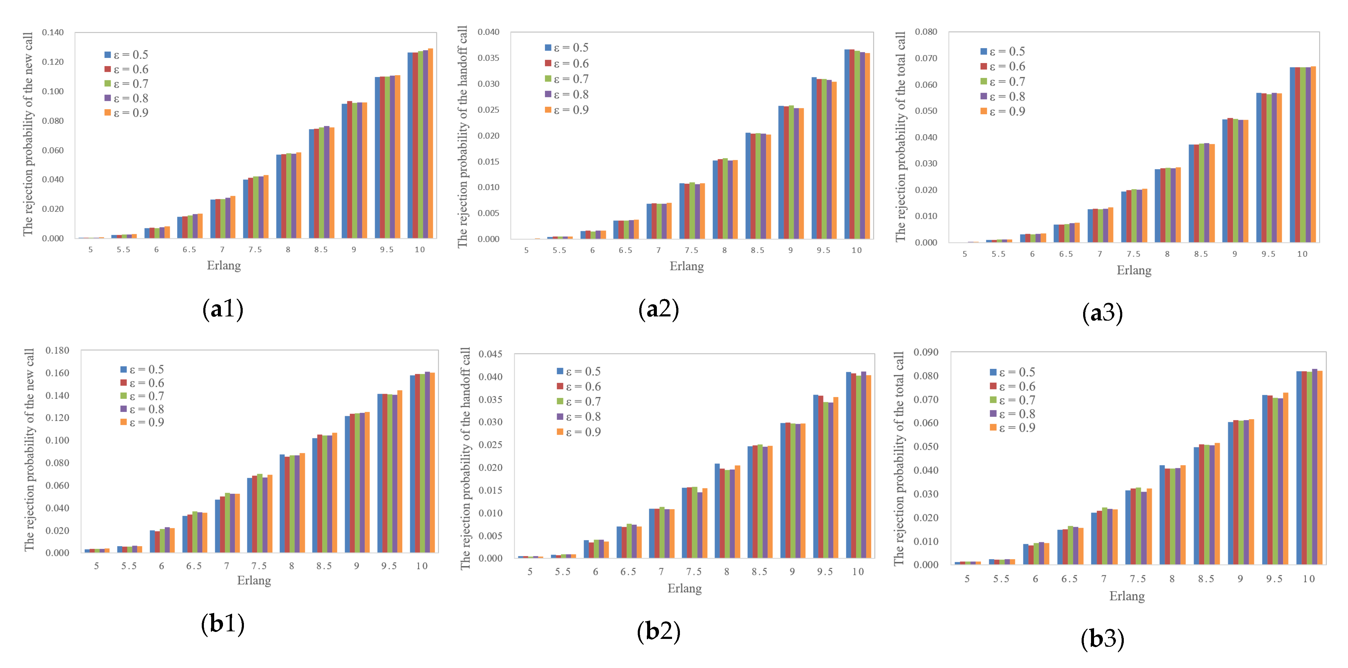
4.2. Results and Analysis

Two simulations were carried out, including the cases of uniform and nonuniform traffic distributions. Under a uniform traffic distribution, the traffic intensity of each cell was the same. Under a nonuniform traffic distribution, the traffic intensity of each cell was different.

Figure 3 shows the comparison results of the four channel allocation algorithms under a uniform traffic distribution with different traffic intensities. It can be seen from Figure 3 that the performances of the different channel allocation algorithms decreased with an increase in the traffic intensity. In terms of the total performance, the RDCA was better than the FCA because the RDCA dynamically allocated eligible channels. The TSCA and SARSA were better than the RDCA. The reason was that RL can learn how to select and perform the actions from a continuous interaction with the environment; thus, the TSCA and SARSA could allocate more appropriate channels to the calls. The rejection probability of a new call with the TSCA was higher than SARSA. That was because the TSCA allocated more eligible channels to the handoff calls and the remaining eligible channels for the new calls were reduced. The rejection probability of a handoff call with the TSCA was much lower than that of the other algorithms. That was because the TSCA made full use of the temporal–spatial correlation of the handoff calls and allocated the eligible channels to the handoff calls. The rejection probabilities of a total call of the TSCA and SARSA were almost the same because they all performed optimal actions in real-time to allocate appropriate channels.

Figure 4 shows a case of a nonuniform traffic distribution. The numbers in the hexagons were the traffic distribution proportions of each cell. Value 1 represented the standard traffic distribution proportion and its traffic intensity was equal to 5.

Figure 5 shows the comparison results of the four channel allocation algorithms under a nonuniform traffic distribution with different traffic intensities. It can be seen from Figure 5 that the performances of the different channel allocation algorithms decreased with an increase in the average traffic intensity. The performances of the four algorithms under a nonuniform traffic distribution were generally worse than that under a uniform traffic distribution.

The performance of the same algorithm under different traffic distributions can be seen in Figure 3 and Figure 5. It can be seen from Figure 3a and Figure 5a that the advantage of a dynamic channel allocation was clearly reflected under a nonuniform traffic distribution. For instance, the rejection probability of a new call of the FCA was 2.4% higher than that of a uniform traffic distribution and the RDCA was 1.5% higher than that of a uniform traffic distribution at 10 Erlangs. In other words, the rejection probability of a new call of the FCA under a nonuniform traffic distribution was 19.98% higher than that under a uniform traffic distribution at 10 Erlangs and the rejection probability of a new call of the RDCA under a nonuniform traffic distribution was 12.74% higher. It can be seen from Figure 3b and Figure 5b that the rejection probability of a handoff call of SARSA under a nonuniform traffic distribution was 18.17% higher than that under a uniform traffic distribution at 10 Erlangs and the rejection probability of a handoff call of the TSCA under a nonuniform traffic distribution was 11.04% higher. The TSCA not only had the lowest rejection probability of a handoff call, but also played a significant role in the performance, especially under a nonuniform traffic distribution and a high traffic intensity. As the TSCA considered the temporal–spatial correlation of the handoff calls, it dynamically allocated more appropriate channels for the handoff calls than SARSA.

The performance of the different a”gori’hms under the same traffic distribution can be seen in Figure 3 and Figure 5. It can be seen from Figure 3b and Figure 5b that the rejection probability of a handoff call of the TSCA was 40.59% lower than that of SARSA under a nonuniform traffic distribution at 10 Erlangs. In the case of a uniform traffic distribution, the rejection probability of a handoff call of the TSCA was 36.68% lower than that of SARSA at 10 Erlangs. It can be seen from Figure 3c and Figure 5c that the rejection probability of a total call of the TSCA was 9.3% lower than that of SARSA at 10 Erlangs under a nonuniform traffic distribution. In the case of a uniform traffic distribution, the rejection probability of a total call of the TSCA was 0.8% lower than that of SARSA at 10 Erlangs. The TSCA improved the performance of the handoff calls, especially under a nonuniform traffic distribution and a high traffic intensity. The TSCA was better than SARSA, especially under a nonuniform traffic distribution.

The RDCA was better than the FCA because the FCA did not have enough channels in high traffic cells and then rejected the calls. The TSCA and SARSA were better than the RDCA. The reason was that RL performs actions in real-time to obtain more benefits from the environment during the iterative process. The TSCA was better than SARSA because the TSCA had a policy considering the temporal–spatial correlation of the handoff calls.

4.3. Parameter Discussion

First, the effect of the change of the parameter ε on the performance of the TSCA was discussed. Five values of the parameter (0.5, 0.6, 0.7, 0.8 and 0.9) were selected. Figure 6 shows the result after using the above values for the proposed algorithm. Simulations were carried out under uniform and nonuniform traffic distributions. It could be seen that the various rejection probabilities fluctuated in the range of one thousandth and the fluctuation was irregular. Therefore, we concluded that the proposed algorithm was insensitive to a parameter value of epsilon.

We then discussed the effect of the change of the parameter γ on the performance of the TSCA. In addition to the previous experience value of 0.845, five different values of the parameter (0.95, 0.85, 0.75, 0.65 and 0.55) were selected. Figure 7 shows the result after using the above values for the proposed algorithm. Simulations were carried out under uniform and nonuniform traffic distributions. The results related to the various rejection probabilities fluctuated in the range of one thousandth and the fluctuation was also irregular. Therefore, we concluded that the proposed algorithm was insensitive to a parameter value of gamma.

5. Conclusions

Frequent handoffs bring a new challenge of designing a reasonable channel allocation algorithm for LEO satellite networks. EC provides sufficient computing power for LEO satellite networks and makes it possible for the application of reinforcement learning. An adaptive DCA algorithm based on a temporal–spatial correlation analysis was proposed in this paper. First, the temporal–spatial correlation of handoff calls was analyzed. Second, the DCA process was formally described as an MDP. Third, a policy for different call events was designed and the MDP model was solved based on SARSA. Finally, simulation experiments were carried out under different traffic distributions and different traffic intensities. The simulation results showed that a TSCA could greatly reduce the rejection probability of handoff calls and improve the total performance of LEO satellite networks. However, the storage space of the Q-values in the TSCA rapidly increased with an increase in the network scale. In the future, we will optimize the required storage space of the proposed algorithm.

References

1. Niephaus, C.; Kretschmer, M.; Ghinea, G. QoS provisioning in converged satellite and terrestrial networks: A survey of the state-of-the-art. IEEE Commun. Surv. Tuts. 2016, 18, 2415–2441. [Google Scholar] [CrossRef]
2. Su, Y.T.; Liu, Y.Q.; Zhou, Y.Q.; Yuan, J.H.; Cao, H.; Shi, J.L. Broadband leo satellite communications: Architectures and key technologies. IEEE Wirel. Commun. 2019, 26, 55–61. [Google Scholar] [CrossRef]
3. Zhang, Z.J.; Zhang, W.Y.; Tseng, F.H. Satellite mobile edge computing: Improving QoS of high-speed satellite-terrestrial networks using edge computing techniques. IEEE Netw. 2019, 33, 70–76. [Google Scholar] [CrossRef]
4. Wang, Y.X.; Yang, J.; Guo, X.Y.; Qu, Z. Satellite edge computing for the internet of things in aerospace. Sensors 2019, 19, 3607. [Google Scholar] [CrossRef] [PubMed] [Green Version]
5. Wei, J.Y.; Han, J.R.; Cao, S.Z. Satellite IoT edge intelligent computing: A research on architecture. Electronics 2019, 8, 1247. [Google Scholar] [CrossRef] [Green Version]
6. Wang, F.; Jiang, D.D.; Qi, S.; Qiao, C.; Shi, L. A dynamic resource scheduling scheme in edge computing satellite networks. Mobile Netw. Appl. 2021, 26, 597–608. [Google Scholar] [CrossRef]
7. Wang, S.H.; Ding, S.T.; Chen, C. Edge computing enabled video segmentation for real-time traffic monitoring in internet of vehicles. Patten Recogn. 2022, 121, 108146. [Google Scholar]
8. Wu, Y.R.; Guo, H.F.; Chakraborty, C. Edge Computing Driven Low-Light Image Dynamic Enhancement for Object Detection. IEEE Trans. Netw. Sci. Eng. 2022. [Google Scholar] [CrossRef]
9. Wu, Y.R.; Zhang, L.L.; Berretti, S. Medical Image Encryption by Content-aware DNA Computing for Secure Healthcare. IEEE Trans. Industr. Inform. 2022, 1–9. [Google Scholar] [CrossRef]
10. Xu, F.M.; Yang, F.; Zhao, C.L.; Wu, S. Deep reinforcement learning based joint edge resource management in maritime network. China Commun. 2022, 5, 211–222. [Google Scholar] [CrossRef]
11. Zhou, J.; Ye, X.G.; Pan, Y.; Xiao, F.; Sun, L.J. Dynamic channel reservation scheme based on priorities in LEO satellite systems. J. Syst. Eng. Electron. 2015, 26, 1–9. [Google Scholar] [CrossRef]
12. Moscholios, L.D.; Vassilakis, V.G.; Sagias, N.C.; Logothetis, M.D. On channel sharing policies in LEO mobile satellite systems. IEEE T. Aerosp. Electron. Syst. 2018, 54, 1628–1640. [Google Scholar] [CrossRef] [Green Version]
13. Chen, S.Z.; Sun, S.H.; Kang, S.L. System integration of terrestrial mobile communication and satellite communication–the trends, challenges and key technologies in B5G and 6G. China Commun. 2020, 17, 156–171. [Google Scholar] [CrossRef]
14. Liu, J.J.; Shi, Y.P.; Fadlullah, Z.M.; Kato, N. Space-air-ground integrated network: A survey. IEEE Commun. Surv. Tutor. 2018, 20, 2714–2741. [Google Scholar] [CrossRef]
15. Mnih, V.; Kavukcuoglu, K.; Silver, D.; Rusu, A.A.; Veness, J.; Bellemare, M.G.; Graves, A.; Riedmiler, M. Human-level control through deep reinforcement learning. Nature 2015, 518, 529–533. [Google Scholar] [CrossRef]
16. Du, J.; Jiang, C.X.; Wang, J.; Ren, Y.; Yu, S.; Han, Z. Resource allocation in space multiaccess systems. IEEE Trans. Aerosp. Electron. Syst. 2017, 53, 598–618. [Google Scholar] [CrossRef]
17. He, D.J.; You, P.; Yong, S.W. Mobility management in LEO satellite communication networks. Chines Space Sci. Technol. 2016, 36, 1–14. [Google Scholar]
18. Kato, N.; Fadlullah, Z.M.; Tang, F.X.; Mao, B.M.; Tani, S.; Okamura, A.; Liu, J.J. Optimizing space-air-ground integrated networks by artificial intelligence. IEEE Wirel. Commun. 2019, 26, 140–147. [Google Scholar] [CrossRef] [Green Version]
19. Del Re, E.; Fantacci, R.; Giambene, G. Handover queuing strategies with dynamic and fixed channel allocation techniques in low earth orbit mobile satellite systems. IEEE Trans. Commun. 1999, 47, 89–102. [Google Scholar] [CrossRef]
20. Li, Y.T.; Wang, S.; Zhou, W.Y. A novel dynamic resource optimization method in LEO-MSS downlink with multi-service based on handover forecasting. In Proceedings of the 5th International Conference Computer and Communications (ICCC), Chengdu, China, 9 June 2019; pp. 809–814. [Google Scholar]
21. Liu, S.J. The Research on Dynamic Resource Management Techniques for Satellite Communication System; Beijing University of Posts and Telecommunications: Beijing, China, 2018. [Google Scholar]
22. Nie, J.H.; Haykin, S. A Q-learning-based dynamic channel assignment technique for mobile communication systems. IEEE Trans. Veh. Technol. 1999, 48, 1676–1687. [Google Scholar]
23. Hu, X.; Liu, S.J.; Chen, R.; Wang, W.D.; Wang, C.T. A deep reinforcement learning-based framework for dynamic resource allocation in multibeam satellite systems. IEEE Commun. Lett. 2018, 22, 1612–1615. [Google Scholar] [CrossRef]
24. Liu, S.J.; Hu, X.; Wang, W.D. Deep reinforcement learning based dynamic channel allocation algorithm in multibeam satellite systems. IEEE Access 2018, 6, 15733–15742. [Google Scholar] [CrossRef]
25. Zheng, F.; Pi, Z.; Zhou, Z.; Wang, K.Z. Leo satellite channel allocation scheme based on reinforcement learning. Mob. Inf. Syst. 2020, 2020, 8868888. [Google Scholar] [CrossRef]
26. Wang, J.; Sun, L.J.; Zhou, J.; Han, C. A dynamic channel reservation strategy based on priorities of multi-traffic and multi-user in LEO satellite networks. J. Circuit. Syst. Comp. 2020, 29, 2050082. [Google Scholar] [CrossRef]
27. Maral, G.; Restrepo, J.; Del Re, E. Performance analysis for a guaranteed handover service in an LEO constellation with a ‘satellite-fixed cell’ system. IEEE Trans. Veh. Technol. 1998, 47, 1200–1214. [Google Scholar] [CrossRef]
28. Del Re, E. Different queuing policies for handover requests in low earth orbit mobile satellite systems. IEEE Trans. Veh. Technol. 1999, 48, 448–458. [Google Scholar] [CrossRef]
29. Deng, B.Y.; Jiang, C.X.; Yao, H.P. The next generation heterogeneous satellite communication of resource management and deep reinforcement learning. IEEE Wirel. Commun. 2020, 27, 105–111. [Google Scholar] [CrossRef]
30. Shi, G.C.; Wu, Y.R.; Liu, J. Incremental Few-Shot Semantic Segmentation via Embedding Adaptive-Update and Hyper-class Representation. arXiv 2022. [Google Scholar] [CrossRef]
31. Zhou, J.; Han, T.T.; Xiao, F. Multi-scale network traffic prediction method based on deep echo state network for internet of things. IEEE Internet Things J. 2022, 9, 21862–21874. [Google Scholar] [CrossRef]
32. Luong, N.C.; Hoang, D.T.; Gong, S.M.; Niyato, D.; Wang, P.; Liang, Y.C.; Kim, D. Applications of deep reinforcement learning in communications and networking: A survey. IEEE Commun. Surv. Tutor. 2019, 21, 3133–3174. [Google Scholar] [CrossRef] [Green Version]
33. Puterman, M.L. Markov Decision Processes: Discrete Stochastic Dynamic Programming; John Wiley & Sons: New York, USA, 2014. [Google Scholar]
34. Alfakin, T.; Hassan, M.M.; Gumae, A.; Savaglio, C.; Fortino, G. Task offloading and resource allocation for mobile edge computing by deep reinforcement learning based on SARSA. IEEE Access 2020, 8, 54074–54084. [Google Scholar] [CrossRef]
35. Liu, C.F.; Bennis, M.; Debbah, M.; Vincent, P. Dynamic task offloading and resource allocation for ultra-reliable low-latency edge computing. IEEE Trans. Commun. 2019, 67, 4132–4150. [Google Scholar] [CrossRef] [Green Version]
36. Lilith, N.; Dogancay, K. Reduced-state SARSA featuring extended channel reassignment for dynamic channel allocation in mobile cellular networks. LNCS 2005, 3421, 531–542. [Google Scholar]
37. Torstein, S. Contributions to Centralized Dynamic Channel Allocation Reinforcement Learning Agents; Norwegian University of Science and Technology: Trondheim, Norway, 2018. [Google Scholar]
38. Zou, Q.Y.; Zhu, L.D. Dynamic channel allocation strategy of satellite communication systems based on grey prediction. In Proceedings of the International Symposium on Networks, Computers and Communications (ISNCC), Istanbul, Turkey, 18–20 June 2019; pp. 1–5. [Google Scholar]
39. Lima, M.A.; Araujo, A.F.; Cesar, A.C. Adaptive genetic algorithms for dynamic channel assignment in mobile cellular communication systems. IEEE Trans. Veh. Technol. 2007, 56, 2685–2696. [Google Scholar] [CrossRef]
40. Lilith, N.; Dogancay, K. Dynamic channel allocation for mobile cellular traffic using reduced-state reinforcement learning. In Proceedings of the Wireless Communications & Networking Conference (WCNC), Atlanta, GA, USA, 21–25 March 2004; pp. 2195–2200. [Google Scholar]
41. Wang, Z.P.; Mathiopoulos, P.T.; Schober, R. Performance analysis and improvement methods for channel resource management strategies of leo-mss with multiparty traffic. IEEE Trans. Veh. Technol. 2008, 57, 3832–3842. [Google Scholar] [CrossRef]
Figure 1. The mobility model of the users.
Applsci 12 10939 g001
Figure 2. Reallocation for a handoff call event. (a) The handoff call occurs; (b) option 1: no reallocation; (c) option 2: reallocate to the call on ch3; (d) option 3: reallocate to the call on ch4.
Applsci 12 10939 g002
Figure 3. Performance comparison under uniform traffic distributions. (a) The rejection probability of the new call; (b) the rejection probability of the handoff call; (c) the rejection probability of the total call.
Applsci 12 10939 g003
Figure 4. Nonuniform traffic distribution in cells.
Applsci 12 10939 g004
Figure 5. Performance comparison under nonuniform traffic distribution. (a) The rejection probability of the new call; (b) the rejection probability of the handoff call; (c) the rejection probability of the total call.
Applsci 12 10939 g005aApplsci 12 10939 g005b
Figure 6. Performance comparison of TSCA with different values of epsilon. (a1) The rejection probability of the new call under uniform distribution; (a2) the rejection probability of the handoff call under uniform distribution; (a3) the rejection probability of the total call under uniform distribution; (b1) the rejection probability of the new call under nonuniform distribution; (b2) the rejection probability of the handoff call under nonuniform distribution; (b3) the rejection probability of the total call under nonuniform distribution.
Applsci 12 10939 g006
Figure 7. Performance comparison of TSCA with different values of gamma. (a1) The rejection probability of the new call under uniform distribution; (a2) the rejection probability of the handoff call under uniform distribution; (a3) the rejection probability of the total call under uniform distribution; (b1) the rejection probability of the new call under nonuniform distribution; (b2) the rejection probability of the handoff call under nonuniform distribution; (b3) the rejection probability of the total call under nonuniform distribution.
Applsci 12 10939 g007