1. Introduction
Lung cancer frequently manifests in the form of a malignant tumor with very high morbidity and mortality worldwide [
1]. In 2015, the World Health Organization integrated multidisciplinary research on lung adenocarcinoma, classifying it into four subtypes based on its different pathologies: atypical adenomatous hyperplasia (AAH), adenocarcinoma in situ (AIS), minimally invasive adenocarcinoma (MIA), and invasive adenocarcinoma (IA).
With advancements in imaging technology, and the widespread application of computed tomography image (CTI) for lung cancer scan, the detection rate of early-stage lung adenocarcinoma, manifested as ground glass nodules (GGNs), has increased significantly. GGNs are closely related to lung cancer, especially lung adenocarcinoma [
2]. During the pathological progress of lung adenocarcinoma from pre-invasive to invasive lesions, GGNs can be observed in the CTI, but lack specificity [
3]. The growth of GGN follows a regular pattern, from benign lesions (e.g., AAH) to malignant lesions (e.g., IA) [
4]. Most GGN lesions are benign, but about 30% are malignant including AIS, MIA, and IA [
5]. However, GGN is likely to be related to other lung diseases such as viral pneumonia [
6], the coronavirus disease 2019 (COVID-19) [
7], etc., where COVID-19 has become a global pandemic. To date, how to distinguish their differences remains a key issue.
In the past, traditional computer-aided diagnosis methods utilize various feature extraction protocols to quantify the appearance of nodules on diagnostic CTIs, and machine learning algorithms such as fuzzy clustering [
8], threshold segmentation [
9], support vector machines [
10], etc., have been employed to classify GGNs. Although these works have achieved impressive performance, extracting appropriate nodule features is very time-consuming, unapparent, and unclear. In recent decades, three classes of remarkable progresses on GGN have been made as follows.
(1) Rapid development in digital imaging and artificial intelligence technologies has led to the field of radiomics, a new technique first proposed by Lambin et al. in 2012 for the noninvasive diagnosis of tumors [
11]. Radiomics is recognized as an effective quantitative tool for characterizing the phenotypes of lung lesion [
12]. It has achieved remarkable results in oncology assessments and diagnosis as well as in post-treatment prognosis [
13]. In early pulmonary nodules diagnosis, for example, studies have demonstrated that radiomics performs well when classifying benign or malignant pulmonary nodules, histopathologic lung cancer phenotypes, and invasiveness in lung adenocarcinoma lesions based on quantitative CTIs [
14,
15].
(2) Deep learning (DL) methods have been demonstrated to greatly reduce the difficulty of feature extraction in CTIs [
16]. Unlike the radiomics model, the DL-based model can extract deep imaging features by using an end-to-end deep convolutional neural network [
17]. Wang et al. [
18] showed that DL combined with the radiomics features could conveniently and automatically obtain the best performance in predicting the invasiveness of lung adenocarcinoma manifesting as GGNs. Moreover, a cascade architecture with both segmentation and classification networks was built. It could perform better and was more stable than the multi-task learning model appearing as GGNs. Ni et al. [
19] proposed an automatic GGN invasiveness classification algorithm for the adenocarcinoma. Experiments showed that the algorithm outperformed the traditional machine learning method.
(3) AI techniques have attracted significant attention in the fight against COVID-19. One crucial application to use CTIs is to segment the COVID-19 infections, which can aid doctors in the treatment. A novel evolvable adversarial framework [
20] has been developed for COVID-19 infection segmentation that incorporated the gradient penalty into the network, penalizing the discriminator’s gradient norm input. Experiments verified that the proposed model achieved superior effectiveness and stability for COVID-19 infection segmentation. Additionally, a weakly supervised method [
21] was proposed for the segmentation of COVID-19 infections in CT slices with scribble supervision. The whole framework was constructed with a mean teacher framework and optimized by a weighted combination of the supervised and unsupervised losses. In the same direction, some other AI methods have been presented for the diagnosis and analysis of COVID-19 [
22], and so on.
Although efforts and progress have been made, existing methods are very limited due to the following two issues:
(1) One-time CTI. The existing studies create their diagnosis models or classifiers based on the set of one-time CTIs, while medical professionals compare the change in GGNs in follow-up CTIs by reviewing and comparing visual characteristics rather than performing a quantitative evaluation. Thus, follow-up CTIs at regular intervals are necessary to identify and track the lesion change.
(2) Poor interpretability. As a data driven algorithm, the development of a DL-based model usually needs a large training dataset with thousands of CTIs. However, the diagnosis and therapy results for these models often have poor interpretability and do not respond to the morphological characteristics in CTIs. In the case of a small scale CTI set, their results may be unreliable. Since these characteristics are often atypical, it makes the differential diagnosis of pathological subtypes based on GGNs even more difficult.
In this paper, we propose a follow-up feature difference-based classification method (FFDC) to improve the accuracy of preoperative diagnosis, and overcome the limitation of the existing one-time feature-based (OFDC) method.
2. Materials and Methods
2.1. Sample Acquisition and Labeling
To build a classifier for the pathological subtypes of GGNs, a set of follow-up CTIs with GGNs must be collected.
The CTIs used in this study were retrospectively collected from the department of pulmonary tumor surgery, Tianjin Medical University General Hospital, corresponding to 146 patients with early lung adenocarcinoma from January 2020 to June 2021. All GGNs were retrospectively labeled by their surgical pathology.
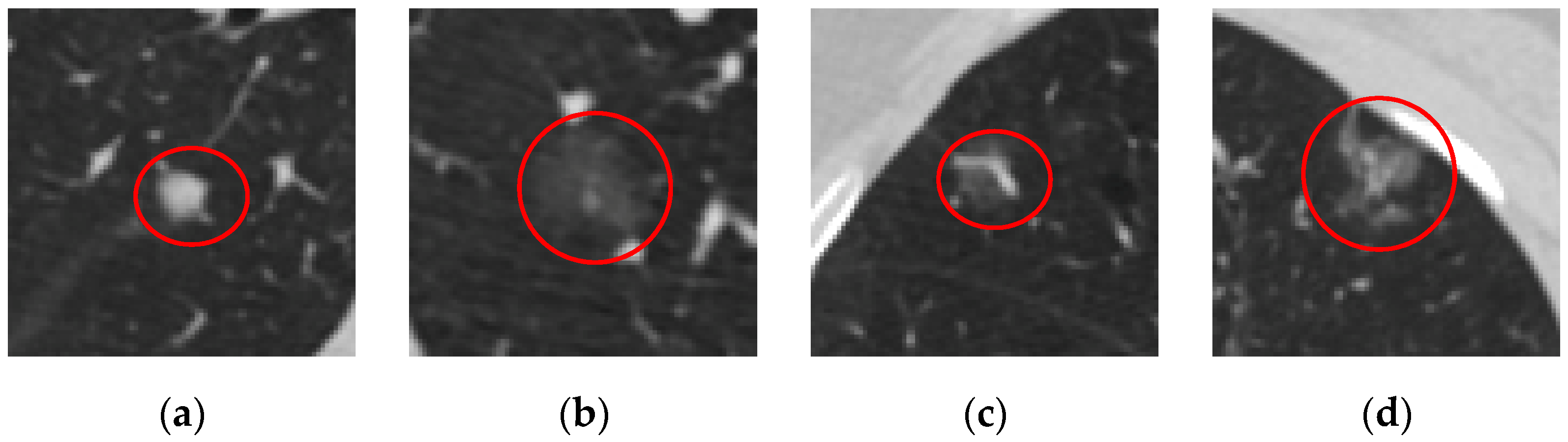
Figure 1 shows the four pathological subtypes of GGNs. All patients had one-time follow-up CTIs at least in which these lesions manifested as GGNs. These GGNs were pathologically analyzed after surgical resection. Hence, their pathological subtypes were confirmed by histopathology analysis. In this paper, the confirmed subtypes were used to label the GGNs for subsequent classification when constructing a classifier. The study was conducted in accordance with the Declaration of Helsinki, and all experiments were approved by the ethics committee of General Hospital of Tianjin Medical University (IRB2020-YX-145-01). The requirement to obtain informed consent from the participants was waived by the ethics committee.
Table 1 shows the number subtypes of 146 patients, their number of follow-ups along these subtypes, and the GGNs subtypes in CTIs, respectively.
In this paper, we implemented the segmentation and feature extraction of GGNs using 3D Slicer [
23]. 3D Slicer is a free and open-source multi-platform software package that is widely used for medical, biomedical, and related imaging research.
Each GGN corresponded to a group of CTIs with different sizes and shapes, but we fixed the CTI with the largest area for sequential classification purposes. According to the pathological and the CT detection reports, each patient’s GGN location and subtype can be found and labeled. The segmentation and labeling steps of GGN are as follows:
- (1)
Import a set of CTIs for each patient into 3D Slicer and locate the GGNs.
- (2)
Select CTIs that contain GGNs and then find the CTI with the largest area among these selected CTIs.
- (3)
Segment the GGN with the largest area and save it as sequential classification.
- (4)
Label the GGNs subtype with pathology reports.
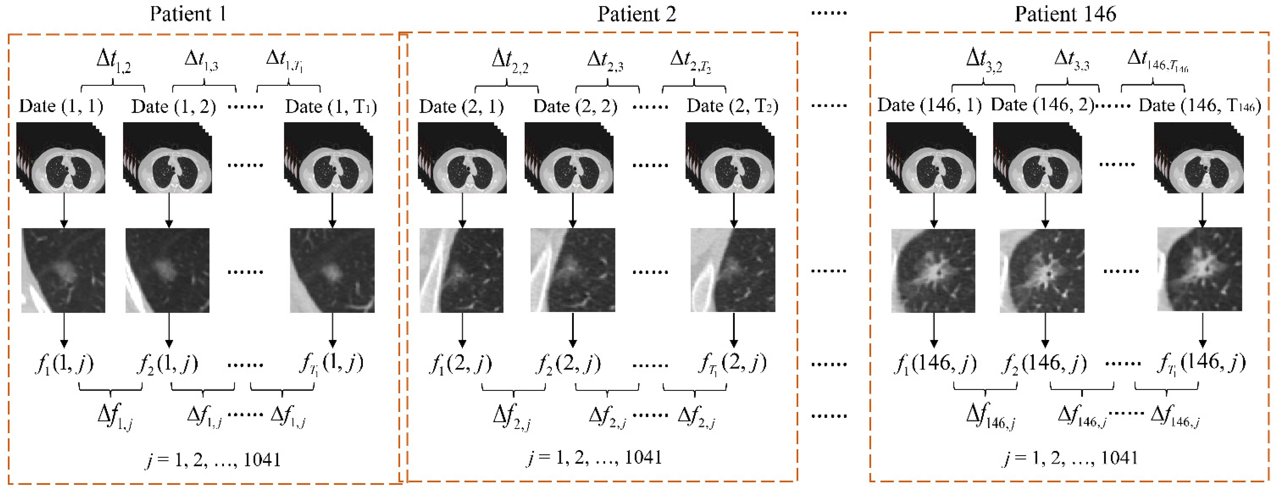
According to 3D Slicer, 1041 features can be extracted from each GGN from the 146 patients’ 386 follow-up CTIs. Algorithmically, let Date (k, i) be the ith follow-up date of kth patient, Δtk,i be the time interval from ith to (i + 1) paired follow-up dates, fk (i, j) be the jth extracted feature from GGN in the ith follow-up CTI, and Tk is the total number of follow-up times of k-th patient, k = 1, 2, …, 146, i = 1, 2, …, 383, j = 1, 2, …, 1041.
Consequently, their feature differences along the paired follow-ups is computed as
where the denominator of Δ
tij aims to normalize the feature change in two different follow-up time intervals. Hence, the GGN feature changes of different patients at different dates are comparable.
Let SFFDC be the set of all feature-difference samples from Equation (1) in FFDC, and SOFDC be the set of samples in OFDC in which the Tkth time CTI for each patient is used to capture the latest features of GGN. Thus, SFFDC = {Δfk (i, j)}, SOFDC = {fk (Tk, j)}
Figure 2 shows the feature extraction process of our proposed method, where these figures in the third row show CTI samples, and these figures in the fourth row refer to the correspondingly segmented GGNs, respectively.
2.2. Radiomics Feature Extraction
The built-in package Pyradiomics in 3D Slicer can extract the main features of GGNs [
24]. Through an analysis of the contour, direction, and gray value of GGNs, we can not only obtain the existing morphological characteristics, but also quantify the sufficient radiomics characteristics [
25].
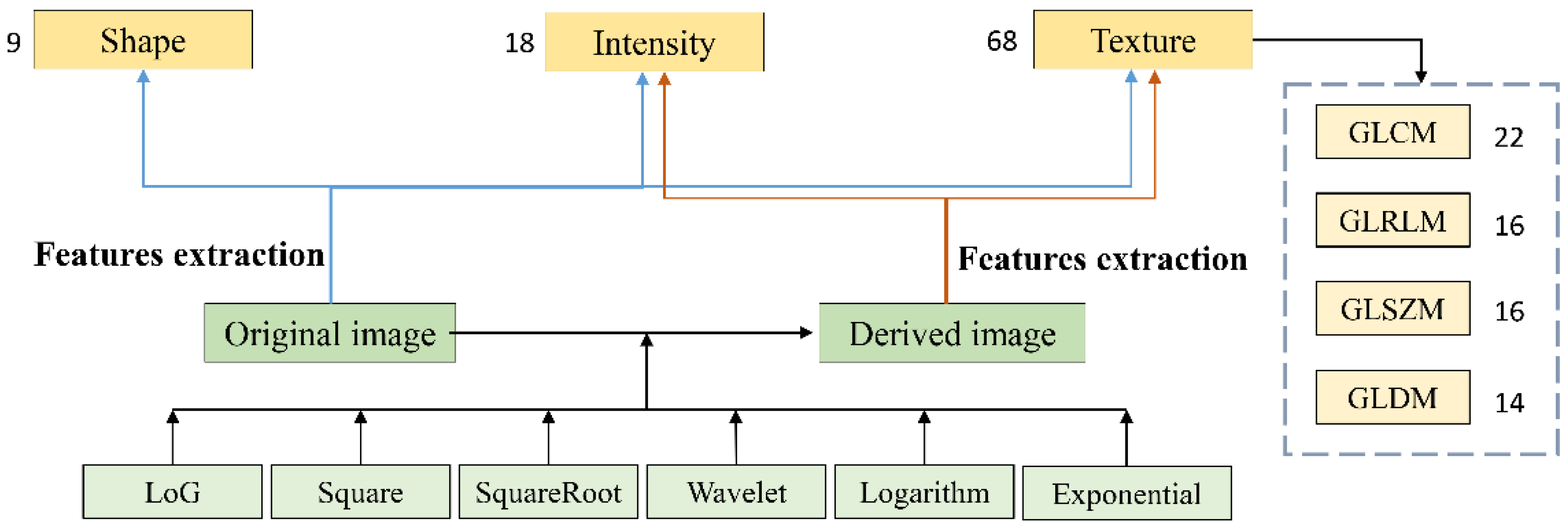
These quantitative features from radiomics are then computed on the original CTI and the six transformation images that follow: square, log, square root, exponential, logarithm, and wavelet. The set of initial features consists of 95 original features, 86 square features, 430 log features, 86 square root features, 172 wavelet features, 86 logarithm features, and 86 exponential features. The original features include nine shape features, 18 histogram features, and 68 texture features. These texture features are further divided into four categories: gray level run length matrix (GLRLM), gray level difference matrix (GLDM), gray level co-occurrence matrix (GLCM), and gray level size zone matrix (GLSZM), with their numbers being 16, 14, 22, and 16, respectively. In addition to the features extracted on the original CTI, we could identify the histogram features and texture features in the derived images.
Figure 3 shows the type and number of 1041 extracted features of GGN for the CTI of each patient.
The pair of CTIs from two-time adjacent flow-up records was used for feature extraction in FFDC from the first to the final follow-ups before the patient was operated, since each patient had two-time follow-up CTIs at least. On the other hand, a patient can have multiple GGNs, and thereby the radiomics feature difference between two-time follow-up CTIs of each GGN is regarded as a sample in FFDC. In contrast, only the most recent CTIs before surgery were used in OFDC. These CTIs had a follow-up period of more than three years compared to the most recent preoperative CTI, which were also referenced as samples and empirically compared for diagnosis in OFDC. In all, 383 samples in FFDC were obtained while 146 samples in OFDC were used.
2.3. Feature Selection and Data Augmentation
When all samples are used for the pathological classification of GGNs, two problems remain, as follows:
- (1)
The number of samples is much less than that of the features, and some features are unnecessary.
- (2)
The sample distribution is imbalanced;
Table 1 shows that the number of samples in the majority class is 96, but there are only eight in the minority class.
To overcome these problems, feature selection and sample augmentation are implemented to
SFFDC and
SOFDC in advance. Feature selection removes irrelevant and redundant features [
26]. To identify the key features and reduce feature dimensionality, we applied the analysis of variance (ANOVA) method [
27]. ANOVA is a single variable analysis method to test whether the effect of any independent feature is obvious for which we computed the three sums of squares in
S,
SST,
SSW, and
SSB [
28]. According to the four pathological subtypes of GGN and all samples, S consists of four groups of {
xij} in which each contains
ni samples,
i = 1, 2, 3, 4;
j = 1, …,
ni.
As a result,
SST is computed by
where
is the mean of all samples in
S.
SSB is computed as
Finally,
SSW is calculated as
To calculate the effect of each feature in
S,
SSB is divided by its freedom degree of 3 to obtain an estimate of
MSB.
SSW is divided by its freedom degree of 233 to obtain an estimate of
MSW. Finally, a statistical value of
F-ratio is computed as
We consulted the priori table of critical F values to obtain a significant p value. In this paper, we took a threshold of 0.05. If p > 0.05, the relative feature is rejected; if not, it is accepted for classification. In the following, the feature selection process is implemented in the IBM SPSS Statistics software. The feature number in S based on FFDC and OFDC was reduced to 142 dimensions and 680 dimensions, respectively.
To overcome the problem of the imbalanced sample distribution in
S, the synthetic minority oversampling technique (SMOTE) [
29,
30] is used to increase the balance radio between cases in four classes in
S. SMOTE randomly creates synthetic samples by adding a weighted difference between the
jth sample and its
k nearest neighbors. This enables oversampling of minority samples. These newly synthesized samples will enhance the generality of the classifiers, thereby avoiding overfitting to a certain extent [
31]. Before data augmentation, all samples in the set on FFDC and the set on OFDC must be normalized according to the following form:
where
Fsta is the standardized feature;
μF is the mean value of the feature; and
σF is the standard deviation of the feature.
According to
Table 1, SMOTE is configured with five nearest neighbors for oversampling to generate synthetic samples in
SFFDC and
SOFDC. The SMOTE steps are as follows:
- (1)
For each sample a in the minority class, five nearest neighbors are found.
- (2)
For each randomly selected nearest neighbor b, a new sample c is constructed with the original sample a according to the following equation:
- (1)
The new sample set is thus obtained by the original and generated samples.
2.4. Performance Assessment
After implementing SMOTE, the number of samples in
SFFDC was extended from 237 to 413, and from 186 to 370 in
SOFDC, as shown in
Table 2. The extended sample set is uniformly denoted as
SS. In this study, we chose macro average arithmetic (MavA), macro average geometric (MavG), and mean F-measure (MFM) as the criteria to evaluate the classification performance [
32]. These criteria have been widely used in multi-class imbalance datasets [
33,
34,
35]. The confusion matrix for binary classification problems is shown in
Table 3.
The confusion matrix represents the results of correctly and incorrectly categorized samples. Here, the positive rate responds to the minority class and the negative to the majority class. In the binary scenario, several common assessment metrics can be derived from the confusion matrix, as shown in
Table 4.
The MavA comprehensively considers the classification results, and each class is assigned the same weight. It calculates the accuracy of each class independently, and then computes their mean to obtain the assessment result. Therefore, the MavA is considered the arithmetic mean of the individual accuracy of each class. MavG is defined as the geometric average of the accuracy for each class. MavA and MavG are formulated as
where TPR
i represents the accuracy rate for the class
i,
i = 1, 2, 3, and 4.
F-measure assigns the same importance degree to recall and precision. It is shown as follows:
The F-measure for two-class classification assessment can be extended to deal with multi-class assessment problems. In this paper, MFM was employed to evaluate the four-category task, defined as follows:
where
i is the index of the class.
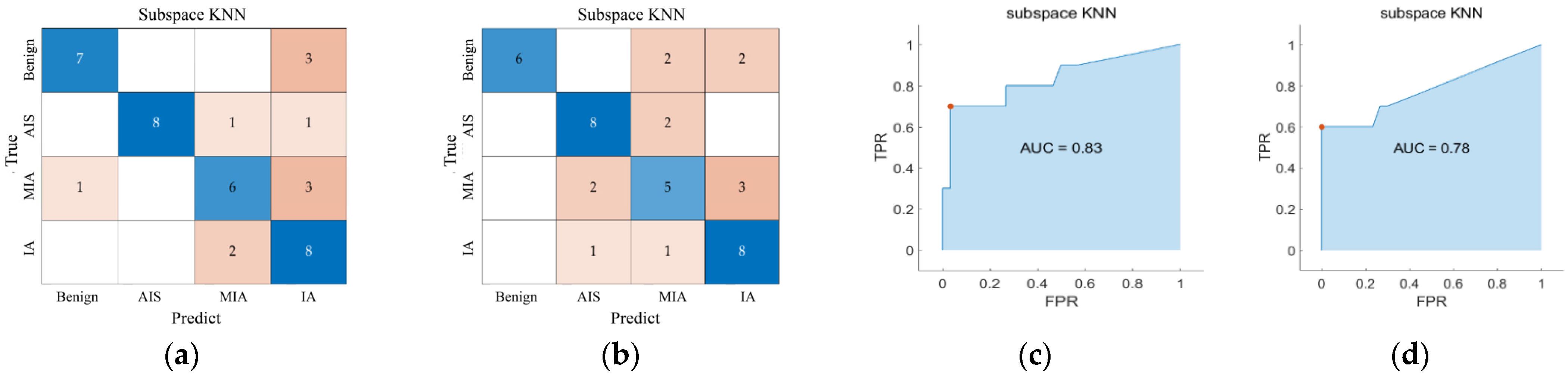
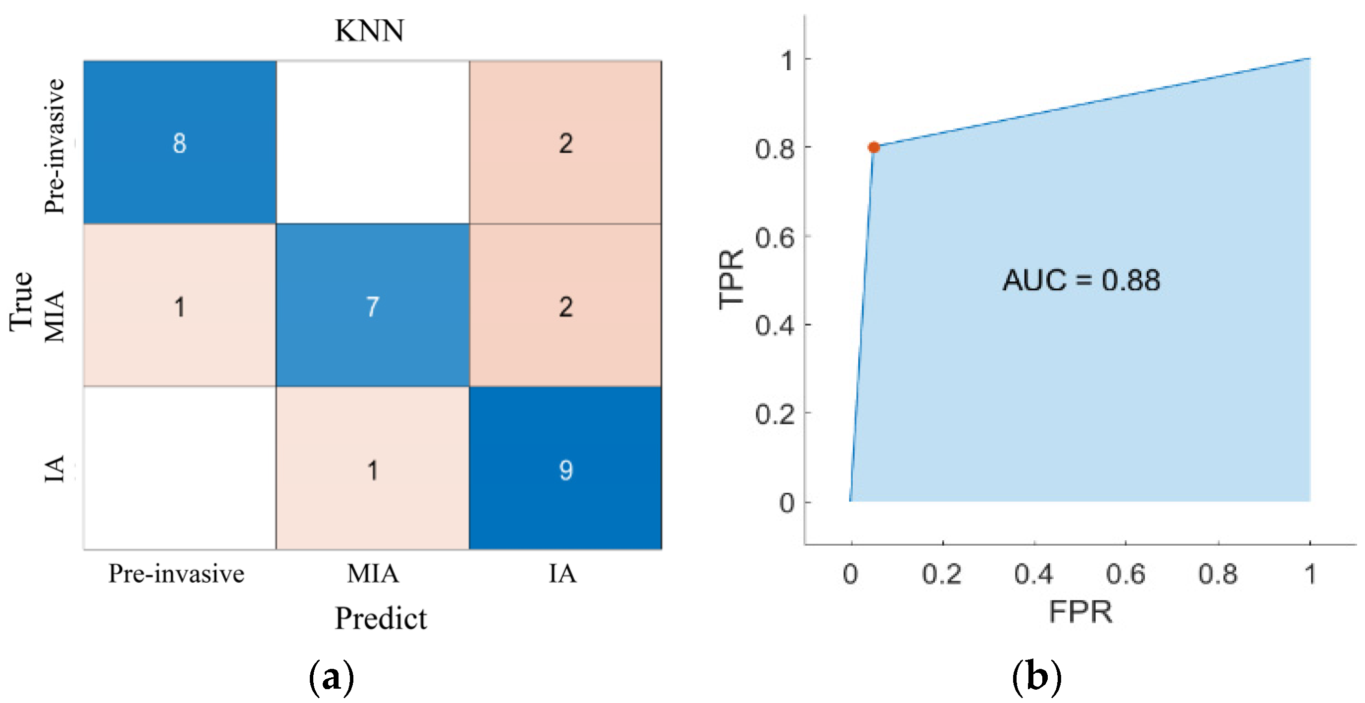
Alternatively, we computed the area under the receiver operating characteristic (ROC) curve, which is also denoted by AUC. In order to extend ROC curve to multi-class classification, the output is binarized. The ROC curve can be drawn by calculating metrics for each label in a one-vs.-all manner and by finding their unweighted mean (macro-averaging).
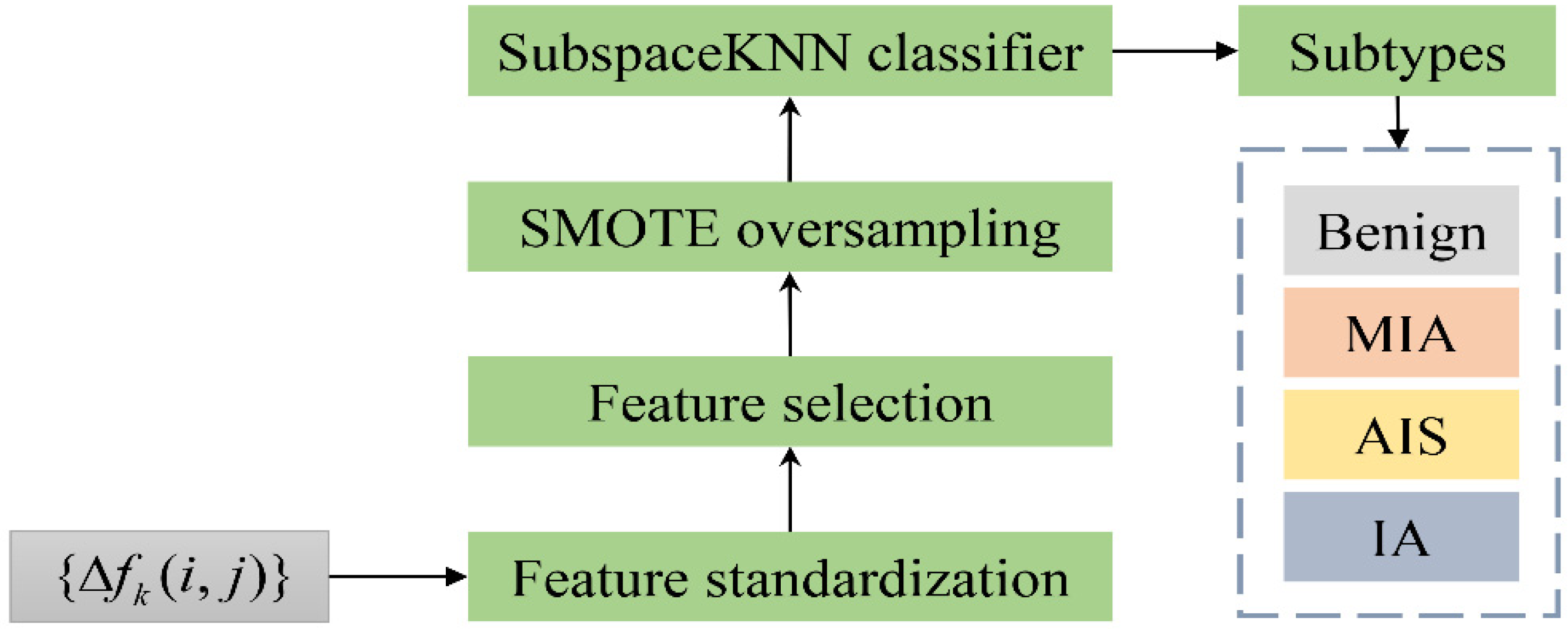
Figure 4 shows the schematic diagram of the FFDC method.
4. Conclusions
This paper presents a new method called FFDC for the classification of four pathological subtypes of GGNs. The radiomics tool was used to extract sufficient and quantitative characteristics. The feature difference of two-time follow-up CTIs was used to find the development of GGNs in different pathological subtypes. The classification results demonstrated the following conclusions.
(1) Feature differences between two-time follow-up CTIs are very helpful for building a more effective classifier after the features of GGN are sufficiently extracted. Based on this, FFDC can achieve a better classification performance than the existing OFDC methods.
(2) Classification of all four pathological subtypes can be effectively realized, while most existing research is focused on the limited three-category radiomics classification.
(3) Four pathological subtypes had significant differences along the three extracted texture characteristics, which proves that the development rate of GGNs can reflect the corresponding pathological stages to a certain extent.
Although FFDC showed clear advantages over the existing OFDC methods, there were still limitations as follows.
(1) GGNs were manually segmented and labeled by posterior pathological analysis reports, but the current focus is machine automatic segmentation and labeling to avoid the error of manual segmentation. Moreover, in clinical applications, when the lesion segmentation is performed by human beings, it has been criticized as time-consuming and generally introducing bias.
(2) Radiomics features were extracted based on the two-dimensional CTI, and the three-dimensional information of the entire GGN lesion must be lost. Generally, the diagnosis model based on three-dimensional GGN segmentation and feature extraction is expected to provide more accurate and stable classifications for lung diseases.
(3) The used machine learning methods such as data argument, subspace classification may fail to give an overall comparison with the current DL algorithm due to the lack of sufficient samples.
How to overcome these problems are our future concerns. For example, the automatic segmentation of GGN lesions is not the research content in this paper, but it will be the focus of our future work.


