

Linear Quadratic Regulator Optimal Control with Integral Action (LQRIC) for LC-Coupling Hybrid Active Power Filter


Abstract
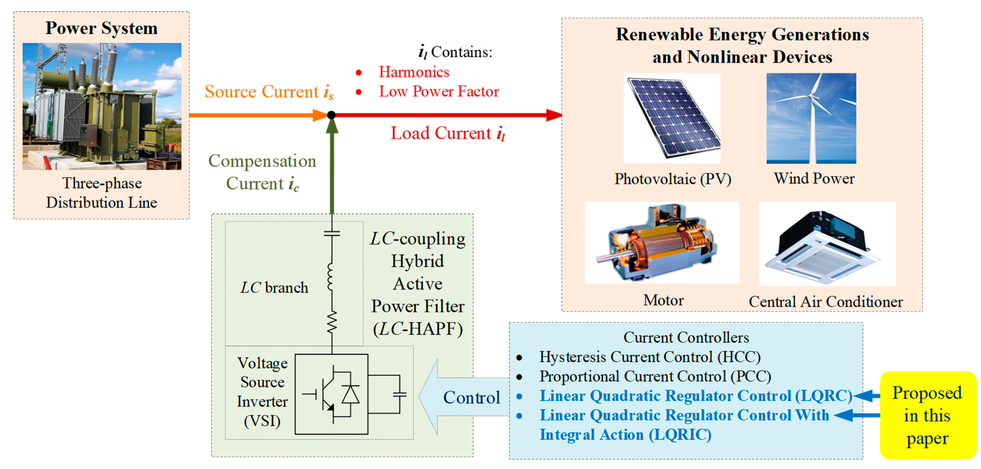
:1. Introduction
- (1)
- A LQRIC for the three-phase four-wire LC-HAPF is proposed to obtain a superior compensation performance.
- (2)
- Design the state-space model in d-q-0 coordinate of a LQRIC-controlled LC-HAPF.
- (3)
- Study the design of the weighting matrices, Q and R, of the LQRIC for LC-HAPF to ensure a good compensation performance.
- (4)
- Compare the simulation results with HCC, PCC and LQRC under different DC-link voltage conditions and verify the effectiveness of the proposed LQRIC for the LC-HAPF.
- (5)
- The experimental results for LQRIC under different DC-link voltages are given to verify the feasibility of the proposed LQRIC.
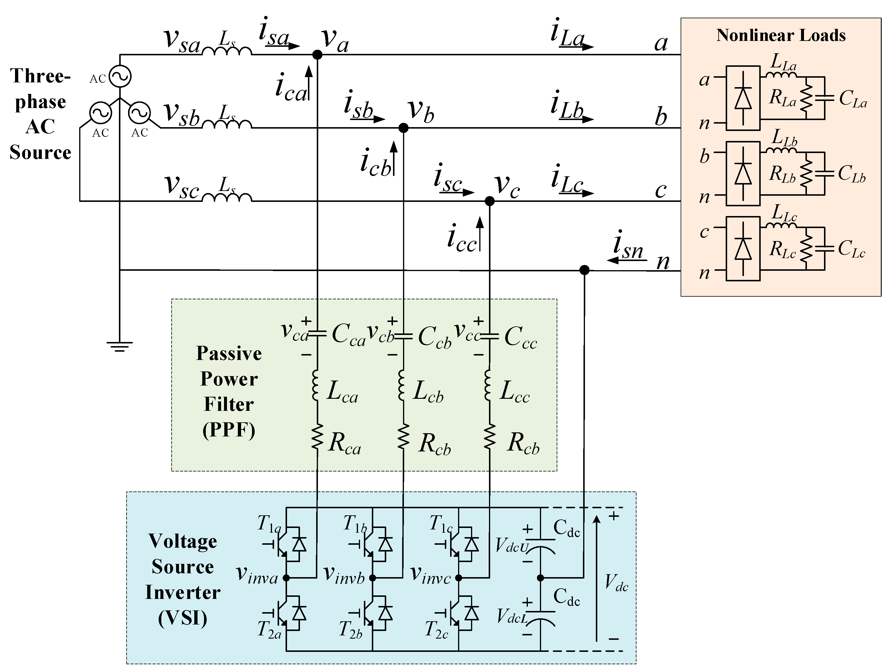
2. Circuit Configuration of LC-HAPF
2.1. Circuit Configuration and System Modeling
2.2. Parameter Design
3. Proposed LQRC and LQRIC for LC-HAPF
3.1. Linear Quadratic Regulator Control (LQRC) for LC-HAPF
3.1.1. State-Space Model for LQRC-Controlled LC-HAPF
3.1.2. LQRC for LC-HAPF
- Select Q and R matrices based on Bryson’s rule;
- Substitute the A, B, Q and R matrices to (18) and obtain the P matrix;
- Using the R, B and P matrices to obtain the optimal control gain K matrix.
3.2. LQRC with Integral Action (LQRIC) for LC-HAPF
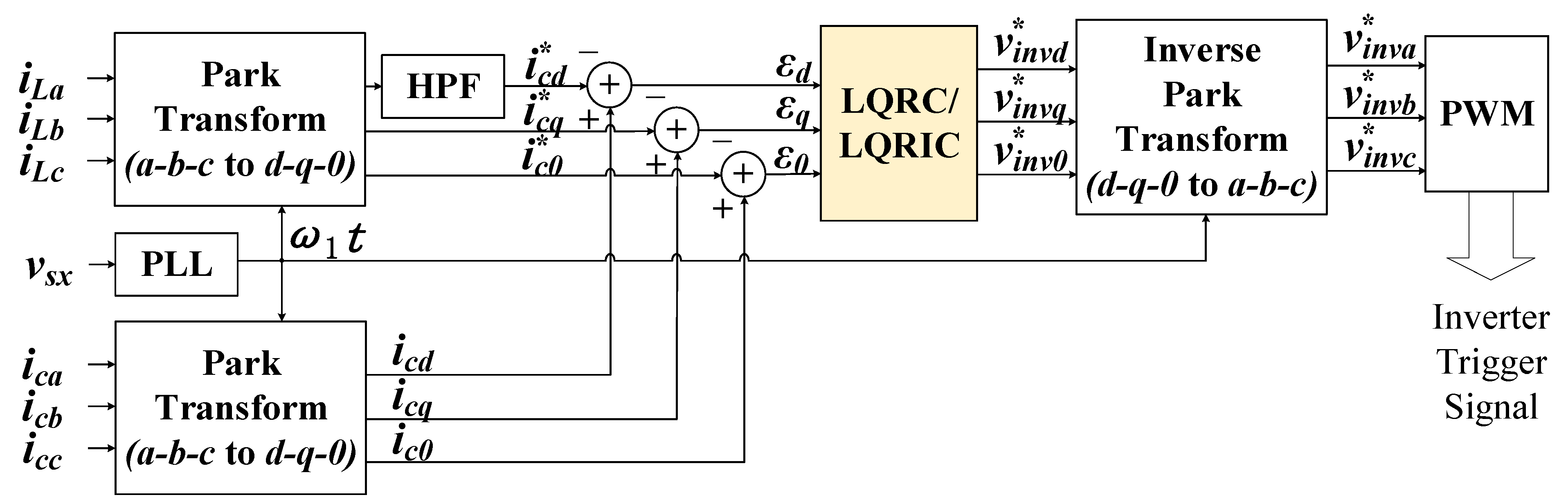
4. Overall Control Strategy of LC-HAPF
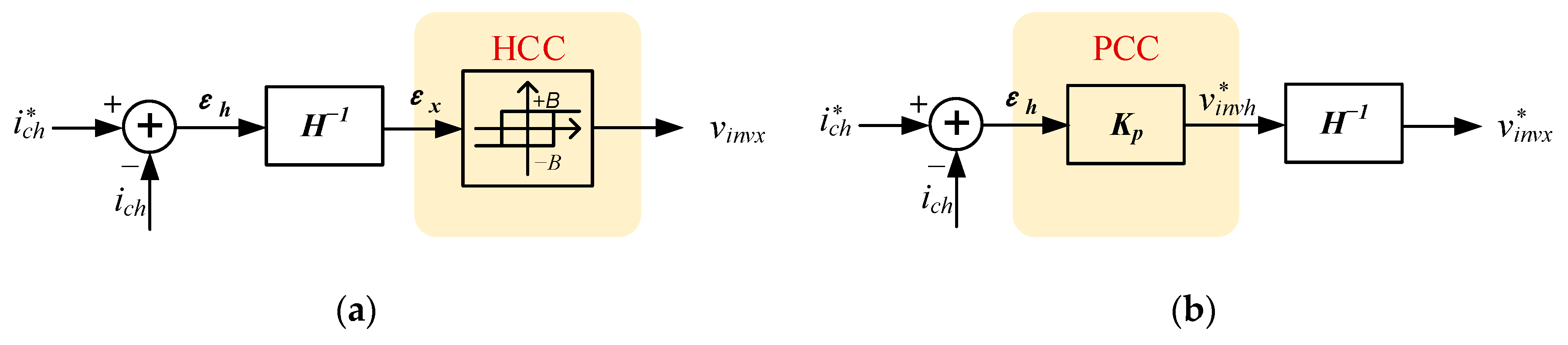
4.1. Hysteresis Current Control (HCC)
4.2. Proportional Current Control (PCC)
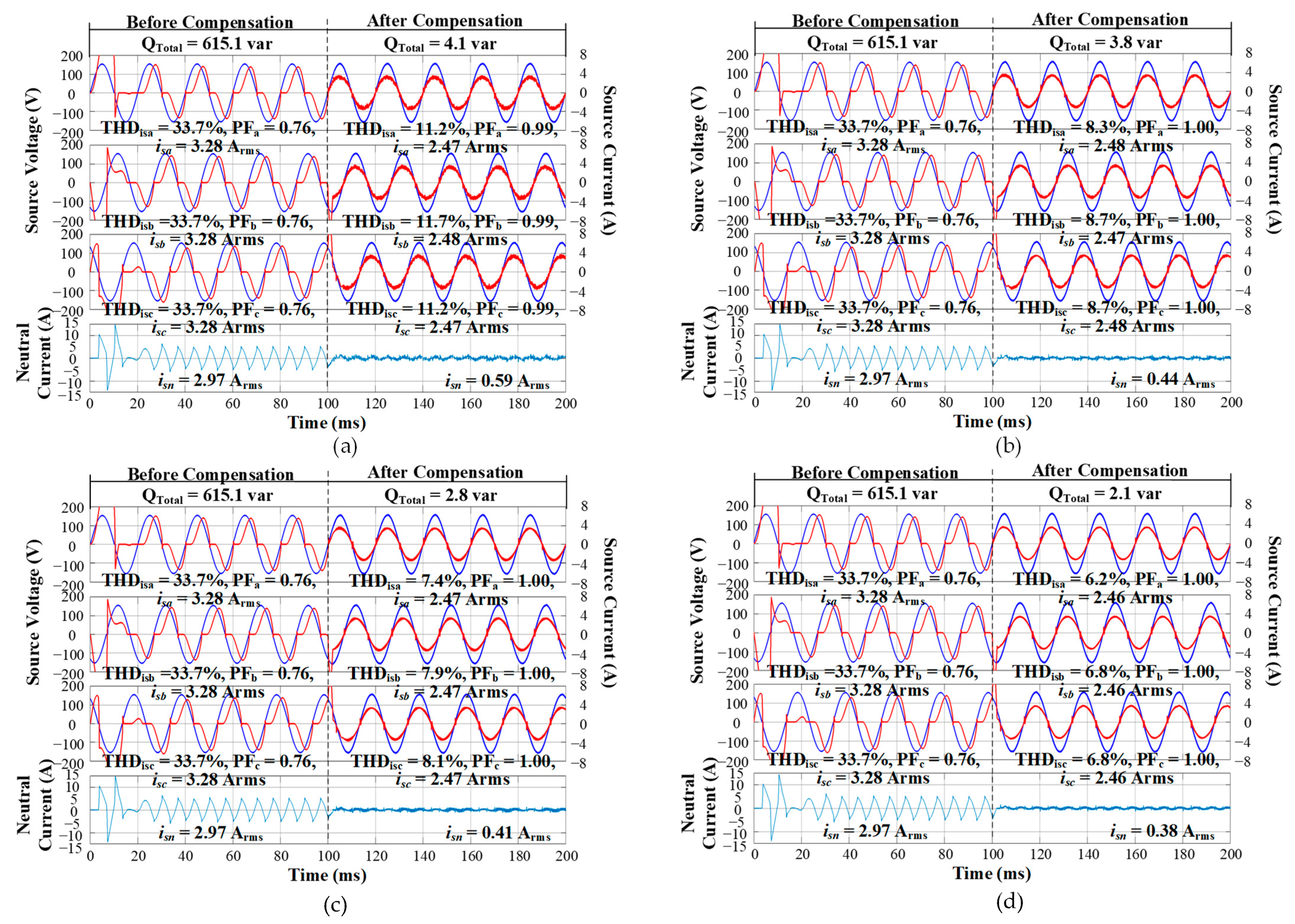
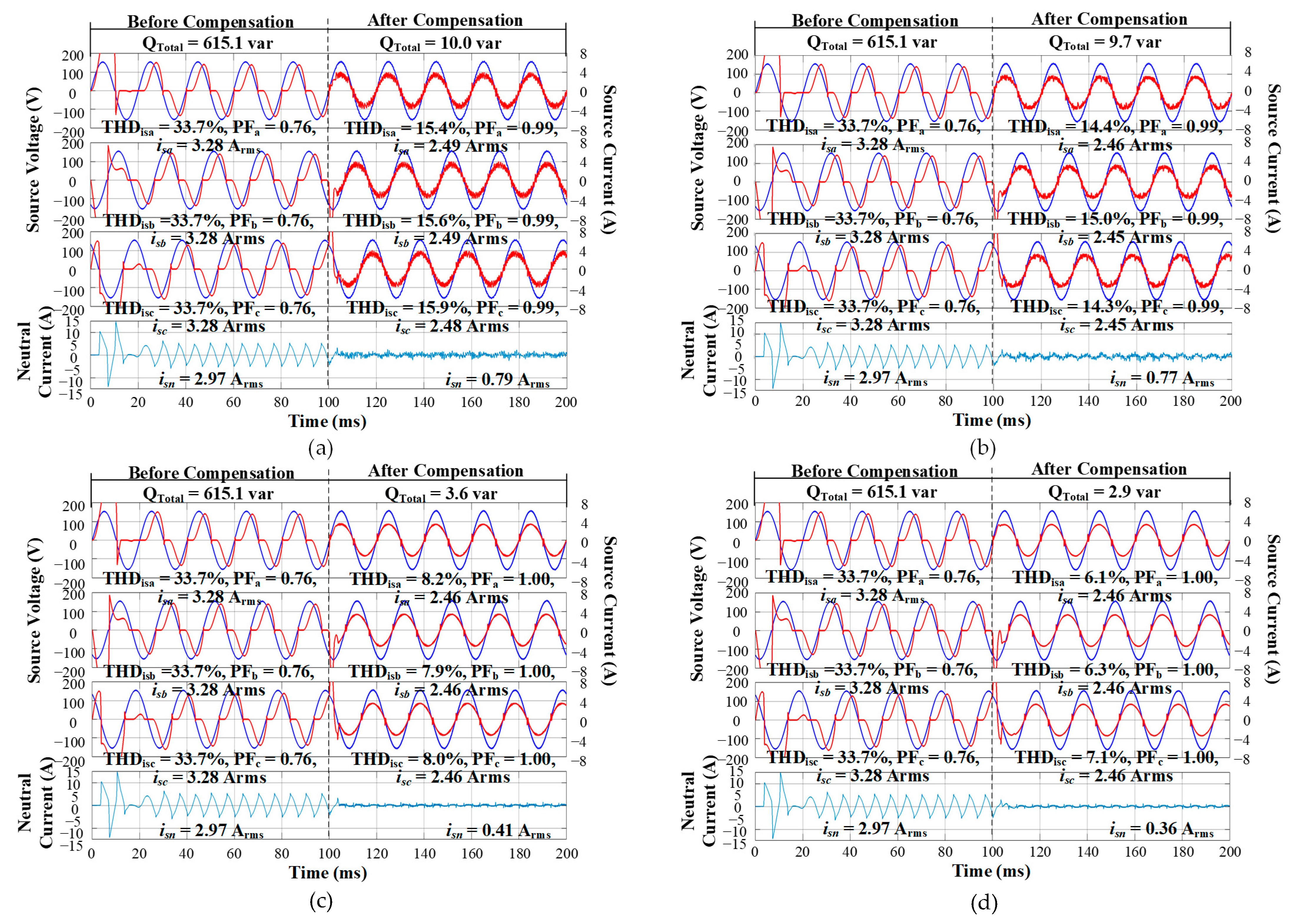
5. Simulation Result
5.1. Hysteresis Current Control (HCC)
5.2. Proportional Current Control (PCC)
5.3. Linear Quadratic Regulator Control (LQRC)
5.4. Proposed LQR Control with Integral Action Control (LQRIC)
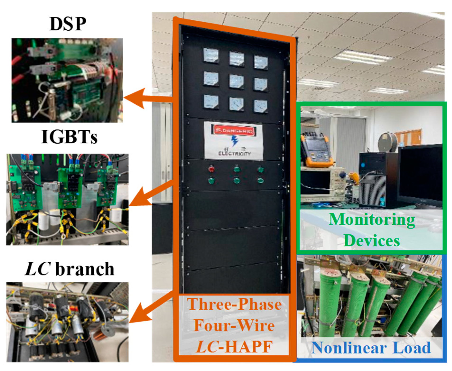
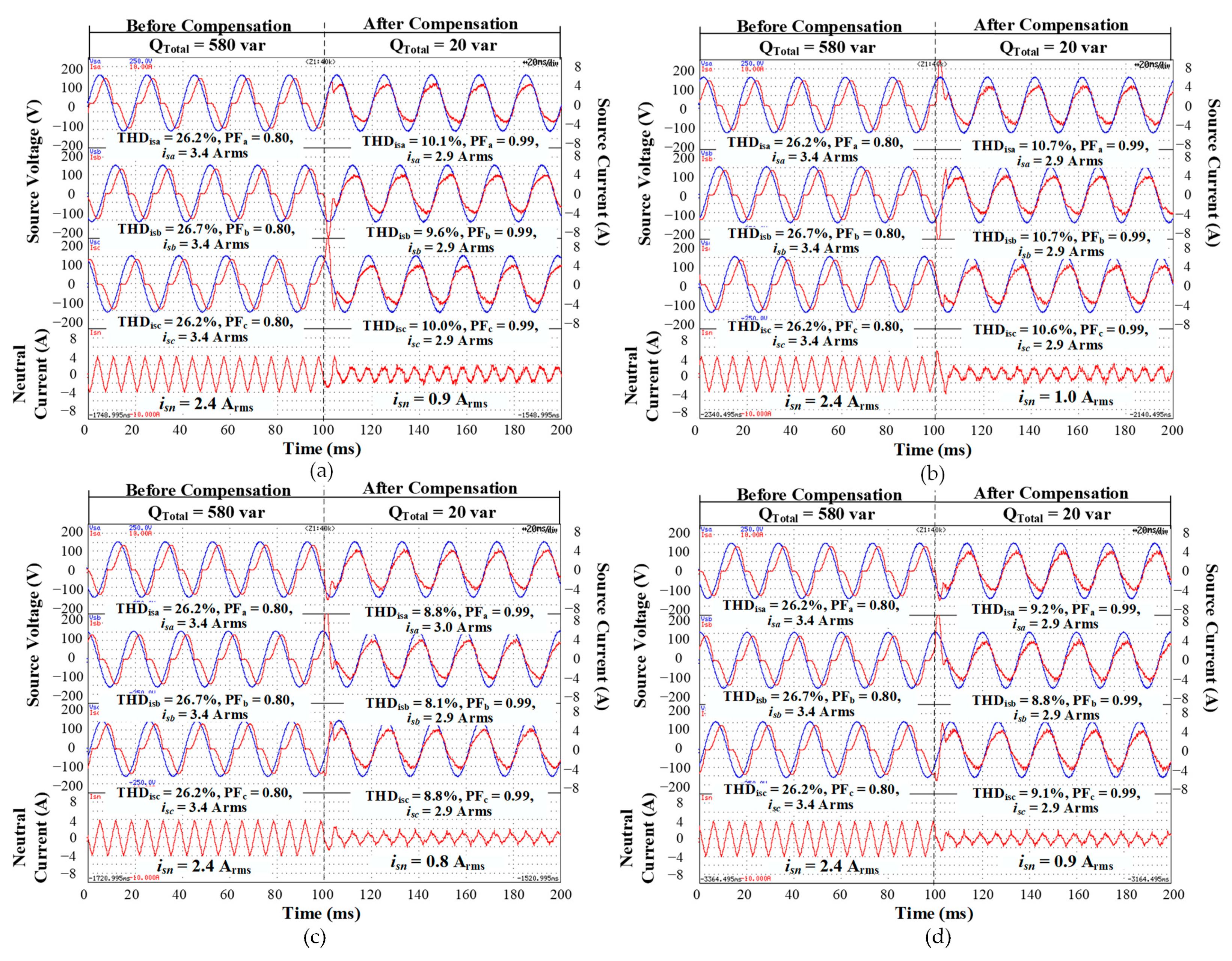
6. Experimental Result
6.1. Linear Quadratic Regulator Control (LQRC)
6.2. Proposed LQR Control with Integral Action Control (LQRIC)
7. Discussion
7.1. Simulation Results Comparison of Different Controllers
7.2. Optimal Control of LQRC and LQRIC
7.3. Feasibility of LQRC and LQRIC Controllers
8. Conclusions
Author Contributions
Funding
Institutional Review Board Statement
Informed Consent Statement
Data Availability Statement
Conflicts of Interest
References
- Farhoodnea, M.; Mohamed, A.; Shareef, H.; Zayandehroodi, H. Power Quality Impact of Grid-Connected Photovoltaic Generation System in Distribution Networks. In Proceedings of the 2012 IEEE Student Conference on Research and Development (SCOReD), Penang, Malaysia, 5–6 December 2012; pp. 1–6. [Google Scholar] [CrossRef]
- Bose, B.K. Power Electronics, Smart Grid, and Renewable Energy Systems. Proc. IEEE. 2017, 105, 2011–2018. [Google Scholar] [CrossRef]
- Di Paolo, M. Analysis of Harmonic Impact of Electric Vehicle Charging on the Electric Power Grid, Based on Smart Grid Regional Demonstration Project—Los Angeles. In Proceedings of the 2017 IEEE Green Energy and Smart Systems Conference (IGESSC), Long Beach, CA, USA, 6–7 November 2017; pp. 1–5. [Google Scholar] [CrossRef]
- Anu, G.; Fernandez, F.M. Identification of Harmonic Injection and Distortion Power at Customer Location. In Proceedings of the 2020 19th International Conference on Harmonics and Quality of Power (ICHQP), Dubai, United Arab Emirates, 6–7 July 2020; pp. 1–5. [Google Scholar] [CrossRef]
- Subjak, J.S.; McQuilkin, J.S. Harmonics-Causes, Effects, Measurements, and Analysis: An Update. IEEE Trans. Ind. Appl. 1990, 26, 1034–1042. [Google Scholar] [CrossRef]
- Das, J.C. Passive Filters-Potentialities and Limitations. IEEE Trans. Ind. Appl. 2004, 40, 232–241. [Google Scholar] [CrossRef]
- Lascu, C.; Asiminoaei, L.; Boldea, I.; Blaabjerg, F. Frequency Response Analysis of Current Controllers for Selective Harmonic Compensation in Active Power Filters. IEEE Trans. Ind. Electron. 2009, 56, 337–347. [Google Scholar] [CrossRef]
- Lam, C.-S.; Wong, M.-C.; Choi, W.-H.; Cui, X.-X.; Mei, H.-M.; Liu, J.-Z. Design and Performance of an Adaptive Low-DC-Voltage-Controlled LC-Hybrid Active Power Filter with a Neutral Inductor in Three-Phase Four-Wire Power Systems. IEEE Trans. Ind. Electron. 2014, 61, 2635–2647. [Google Scholar] [CrossRef]
- Sou, W.-K.; Choi, W.-H.; Chao, C.-W.; Lam, C.-S.; Gong, C.; Wong, C.-K.; Wong, M.-C. A Deadbeat Current Controller of LC-Hybrid Active Power Filter for Power Quality Improvement. IEEE Trans. Emerg. 2020, 8, 3891–3905. [Google Scholar] [CrossRef]
- Gong, C.; Sou, W.-K.; Lam, C.-S. Design and Analysis of Vector Proportional–Integral Current Controller for LC-Coupling Hybrid Active Power Filter with Minimum DC-Link Voltage. IEEE Trans. Ind. Electron. 2021, 36, 9041–9056. [Google Scholar] [CrossRef]
- Chan, P.-I.; Sou, W.-K.; Lam, C.-S. Improved Model Predictive Control with Signal Correction Technique of LC-Coupling Hybrid Active Power Filter. IEEE Trans. Emerg. Sel. Top. Power Electron. 2022, 10, 4650–4664. [Google Scholar] [CrossRef]
- Sou, W.-K.; Chao, C.-W.; Gong, C.; Lam, C.-S.; Wong, C.-K. Analysis, Design, and Implementation of Multi-Quasi-Proportional-Resonant Controller for Thyristor-Controlled LC-Coupling Hybrid Active Power Filter (TCLC-HAPF). IEEE Trans. Ind. Electron. 2022, 69, 29–40. [Google Scholar] [CrossRef]
- Xiang, Z.; Pang, Y.; Wang, L.; Wong, C.-K.; Lam, C.-S.; Wong, M.-C. Design, Control and Comparative Analysis of an LCLC Coupling Hybrid Active Power Filter. IET Power Electron. 2020, 13, 1207–1217. [Google Scholar] [CrossRef]
- Lam, C.-S.; Wong, M.-C.; Han, Y.-D. Hysteresis current control of hybrid active power filters. IET Power Electron. 2012, 5, 1175–1187. [Google Scholar] [CrossRef]
- Ye, T.; Dai, N.; Lam, C.-S.; Wong, M.-C.; Guerrero, J.M. Analysis, Design, and Implementation of a Quasi-Proportional-Resonant Controller for a Multifunctional Capacitive-Coupling Grid-Connected Inverter. IEEE Trans. Ind Appl. 2016, 52, 4269–4280. [Google Scholar] [CrossRef]
- Ahmed, M.; Alsokhiry, F.; Abdel-Khalik, A.S.; Ahmed, K.H.; Al-Turki, Y. Improved Damping Control Method for Grid-Forming Converters Using LQR and Optimally Weighted Feedback Control Loops. IEEE Access 2021, 9, 87484–87500. [Google Scholar] [CrossRef]
- Fan, L.; Liu, P.; Teng, H.; Qiu, G.; Jiang, P. Design of LQR Tracking Controller Combined with Orthogonal Collocation State Planning for Process Optimal Control. IEEE Access 2020, 8, 223905–223917. [Google Scholar] [CrossRef]
- Huerta, F.; Pizarro, D.; Cobreces, S.; Rodriguez, F.J.; Giron, C.; Rodriguez, A. LQG Servo Controller for the Current Control of LCL Grid-Connected Voltage-Source Converters. IEEE Trans. Ind. Electron. 2012, 59, 4272–4284. [Google Scholar] [CrossRef]
- Panigrahi, R.; Subudhi, B.; Panda, P.C. A Robust LQG Servo Control Strategy of Shunt-Active Power Filter for Power Quality Enhancement. IEEE Trans. Power Electron. 2016, 31, 2860–2869. [Google Scholar] [CrossRef]
- Ufnalski, B.; Kaszewski, A.; Grzesiak, L.M. Particle Swarm Optimization of the Multioscillatory LQR for a Three-Phase Four-Wire Voltage-Source Inverter with an LC Output Filter. IEEE Trans. Ind. Electron. 2015, 62, 484–493. [Google Scholar] [CrossRef]
- De Almeida, P.M.; Ribeiro, A.S.B.; Souza, I.D.N.; de Fernandes, M.C.; Fogli, G.A.; Ćuk, V.; Barbosa, P.G.; Ribeiro, P.F. Systematic Design of a DLQR Applied to Grid-Forming Converters. IEEE J. Emerg. Sel. Top. Ind. Electron. 2020, 1, 200–210. [Google Scholar] [CrossRef]
- Zhang, H.; Feng, T.; Liang, H.; Luo, Y. LQR-Based Optimal Distributed Cooperative Design for Linear Discrete-Time Multiagent Systems. IEEE Trans. Neural Netw. Learn. Syst. 2017, 28, 599–611. [Google Scholar] [CrossRef]
- Gokcek, C.; Kabamba, P.T.; Meerkov, S.M. An LQR/LQG Theory for Systems with Saturating Actuators. IEEE Trans. Autom. Control 2001, 46, 1529–1542. [Google Scholar] [CrossRef]
- Kedjar, B.; Al-Haddad, K. LQR with Integral Action to Enhance Dynamic Performance of Three-Phase Three-Wire Shunt Active Filter. In Proceedings of the 2007 IEEE Power Electronics Specialists Conference, Orlando, FL, USA, 17–21 June 2007; pp. 1138–1144. [Google Scholar] [CrossRef]
- Arab, N.; Vahedi, H.; Al-Haddad, K. LQR Control of Single-Phase Grid-Tied PUC5 Inverter with LCL Filter. IEEE Trans. Ind. Electron. 2020, 67, 297–307. [Google Scholar] [CrossRef]
- Kedjar, B.; Al-Haddad, K. DSP-Based Implementation of an LQR With Integral Action for a Three-Phase Three-Wire Shunt Active Power Filter. IEEE Trans. Ind. Electron. 2009, 56, 2821–2828. [Google Scholar] [CrossRef]
- Kedjar, B.; Al-Haddad, K. LQ Control of a Three-Phase Four-Wire Shunt Active Power Filter Based on Three-Level NPC Inverter. In Proceedings of the 2008 Canadian Conference on Electrical and Computer Engineering, Niagara Falls, ON, Canada, 6–7 May 2008; pp. 1297–1302. [Google Scholar] [CrossRef]
- Santiprapan, P.; Areerak, K.; Areerak, K. Dynamic Model of Active Power Filter in Three-Phase Four-Wire System. In Proceedings of the 2014 11th International Conference on Electrical Engineering/Electronics, Computer, Telecommunications and Information Technology (ECTI-CON), Nakhon, Thailand, 14–17 May 2014; pp. 1–5. [Google Scholar] [CrossRef]
- Busatto, T.; Rönnberg, S.; Bollen, M.H.J. Comparison of Models of Single-Phase Diode Bridge Rectifiers for Their Use in Harmonic Studies with Many Devices. Energies 2022, 15, 66. [Google Scholar] [CrossRef]
- Franklin, G.F.; Powell, J.D.; Emami-Naeini, A. Feedback Control of Dynamic Systems, 6th ed.; Pearson: Upper Saddle River, NJ, USA, 2010; ISBN 978-0-13-601969-5. [Google Scholar]
- IEEE Std 519-2014 (Revision of IEEE Std 519-1992); Recommended Practice and Requirements for Harmonic Control in Electric Power Systems. IEEE: Hoboken, NJ, USA, 2014; pp. 1–29. [CrossRef]


| System Parameters | Values | Controller Parameters | Values |
|---|---|---|---|
| vsx, f | 110 Vrms, 50 Hz | H (HCC) | 0.156 |
| Ls | 0.5 mH | Kp (PCC) | 250 |
| LLx, CLx, RLx | 35 mH, 400 μF, 43 Ω | qq1, qq2, qq3, rq1, rq2, rq3 (LQRC) | 350, 310, 370, 0.01, 0.01, 0.01 |
| Lcx, Ccx, Rcx | 8 mH, 50 μF, 0.03 Ω | qq1, qq2, qq3, qq4, qq5, qq6, rq1, rq2, rq3 (LQRIC) | 260, 240, 290, 830, 820, 450, 0.01, 0.01, 0.01 |
| Vdc | 100 V | ||
| fs | 10 kHz |
| Before Compensation | After Compensation | ||||
|---|---|---|---|---|---|
| HCC | PCC | LQRC | LQRIC | ||
| THDisa (%) | 33.7 | 11.3 | 8.3 | 7.4 | 6.2 |
| THDisb (%) | 33.7 | 10.9 | 8.7 | 7.9 | 6.8 |
| THDisc (%) | 33.7 | 11.3 | 8.7 | 8.1 | 6.8 |
| PF | 0.76 | 0.99 | 1.00 | 1.00 | 1.00 |
| QTotal (var) | 615.1 | 4.2 | 3.8 | 2.8 | 2.1 |
| Total SW loss (W) | / | 25.0 | 26.3 | 26.6 | 27.0 |
| isa (Arms) | 3.28 | 2.50 | 2.48 | 2.47 | 2.46 |
| isb (Arms) | 3.28 | 2.50 | 2.47 | 2.47 | 2.46 |
| isc (Arms) | 3.28 | 2.49 | 2.48 | 2.47 | 2.46 |
| isn (Arms) | 2.97 | 0.49 | 0.44 | 0.41 | 0.38 |
| Before Compensation | After Compensation | ||||
|---|---|---|---|---|---|
| HCC | PCC | LQRC | LQRIC | ||
| THDisa (%) | 33.7 | 15.4 | 14.4 | 8.2 | 6.1 |
| THDisb (%) | 33.7 | 15.6 | 15.0 | 7.9 | 6.3 |
| THDisc (%) | 33.7 | 15.9 | 14.3 | 8.0 | 7.1 |
| PF | 0.76 | 0.99 | 0.99 | 1.00 | 1.00 |
| QTotal (var) | 615.1 | 10.0 | 9.7 | 3.6 | 2.9 |
| Total SW loss (W) | / | 12.3 | 13.8 | 15.9 | 15.9 |
| isa (Arms) | 3.28 | 2.49 | 2.46 | 2.46 | 2.46 |
| isb (Arms) | 3.28 | 2.49 | 2.45 | 2.46 | 2.46 |
| isc (Arms) | 3.28 | 2.48 | 2.45 | 2.46 | 2.46 |
| isn (Arms) | 2.97 | 0.79 | 0.77 | 0.41 | 0.36 |
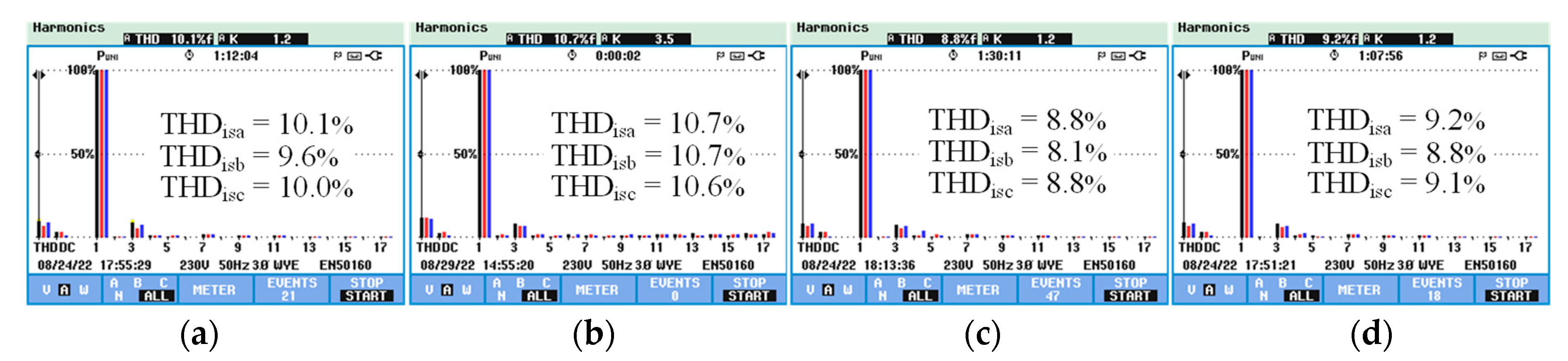
| Before Compensation | 50V DC-Link Voltage | 40V DC-Link Voltage | |||
|---|---|---|---|---|---|
| LQRC | LQRIC | LQRC | LQRIC | ||
| THDisa (%) | 26.2 | 10.1 | 8.8 | 10.7 | 9.2 |
| THDisb (%) | 26.7 | 9.6 | 8.1 | 10.7 | 8.8 |
| THDisc (%) | 26.2 | 10.0 | 8.8 | 10.6 | 9.1 |
| PF | 0.80 | 0.99 | 0.99 | 0.99 | 0.99 |
| QTotal (var) | 580 | 20 | 20 | 20 | 20 |
| Total SW loss (W) | / | 29.6 | 30.2 | 19.5 | 20.3 |
| isa (Arms) | 3.4 | 2.9 | 3.0 | 2.9 | 2.9 |
| isb (Arms) | 3.4 | 2.9 | 2.9 | 2.9 | 2.9 |
| isc (Arms) | 3.4 | 2.9 | 2.9 | 2.9 | 2.9 |
| isn (Arms) | 2.4 | 0.9 | 0.8 | 1.0 | 0.9 |
Publisher’s Note: MDPI stays neutral with regard to jurisdictional claims in published maps and institutional affiliations. |
© 2022 by the authors. Licensee MDPI, Basel, Switzerland. This article is an open access article distributed under the terms and conditions of the Creative Commons Attribution (CC BY) license (https://creativecommons.org/licenses/by/4.0/).
Share and Cite
Hong, Q.-R.; Chan, P.-I.; Sou, W.-K.; Gong, C.; Lam, C.-S. Linear Quadratic Regulator Optimal Control with Integral Action (LQRIC) for LC-Coupling Hybrid Active Power Filter. Appl. Sci. 2022, 12, 9772. https://doi.org/10.3390/app12199772
Hong Q-R, Chan P-I, Sou W-K, Gong C, Lam C-S. Linear Quadratic Regulator Optimal Control with Integral Action (LQRIC) for LC-Coupling Hybrid Active Power Filter. Applied Sciences. 2022; 12(19):9772. https://doi.org/10.3390/app12199772
Chicago/Turabian StyleHong, Qian-Rong, Pak-Ian Chan, Wai-Kit Sou, Cheng Gong, and Chi-Seng Lam. 2022. "Linear Quadratic Regulator Optimal Control with Integral Action (LQRIC) for LC-Coupling Hybrid Active Power Filter" Applied Sciences 12, no. 19: 9772. https://doi.org/10.3390/app12199772