Learning to Optimise a Swarm of UAVs

Abstract

The use of Unmanned Aerial Vehicles (UAVs) has shown a drastic increase in interest in the past few years. Current applications mainly depend on single UAV operations, which face critical limitations such as mission range or resilience. Using several autonomous UAVs as a swarm is a promising approach to overcome these. However, designing an efficient swarm is a challenging task, since its global behaviour emerges solely from local decisions and interactions. These properties make classical multirobot design techniques not applicable, while evolutionary swarm robotics is typically limited to a single use case. This work, thus, proposes an automated swarming algorithm design approach, and more precisely, a generative hyper-heuristic relying on multi-objective reinforcement learning, that permits us to obtain not only efficient but also reusable swarming behaviours. Experimental results on a three-objective variant of the Coverage of a Connected UAV Swarm problem demonstrate that it not only permits one to generate swarming heuristics that outperform the state-of-the-art in terms of coverage by a swarm of UAVs but also provides high stability. Indeed, it is empirically demonstrated that the model trained on a certain class of instances generates heuristics and is capable of performing well on instances with a different size or swarm density.

1. Introduction

The usage of UAVs finds its roots where human intervention might be difficult, risky or costly. Initially thought for military purposes, UAVs have demonstrated their tremendous potential in civilian applications such as parcel delivery, rescue mission or environment monitoring. Current applications nonetheless rely on the usage of a single UAV (remotely piloted or autonomous), which faces multiple limitations, such as its range of action, payload capacity and system resilience.

Using several autonomous UAVs simultaneously as a swarm is one promising solution to address these limitations. Inspired by natural phenomena (e.g., birds flocks or ant colonies), swarm intelligence allows one to achieve complex tasks while solely relying on local decisions and interactions. Such a distributed and self-organised approach allows multi-UAV systems to be more scalable, resilient and flexible.

However, defining a priori the behaviour of each individual swarm member to obtain a desired collective behaviour is difficult and time-consuming due to the high uncertainty of a swarm operation. As a consequence, classical multi-robot design techniques are not applicable, as they require the global specifications of the systems to define the behaviour of individual robots [1]. Other methods, mainly belonging to the field of evolutionary swarm robotics, ref. [2] have been proposed to automate the design of more complex systems like robot swarms. Here, the design problem is modelled as an optimisation problem which consists in finding an optimal parameterisation and architecture of the neural network used to control each swarm member. However, as outlined in [3], these have limitations, for instance, they are typically applied to a single use case (i.e., no generalisation study).

Automating the design of flexible/reusable swarming behaviours would, thus, overcome these challenges. However, as outlined by Birattari et al. [1], automatic robot swarm design still remains an open research problem.

The work proposed in this article, thus, aims to automate the design phase of UAV swarms thanks to a novel hyper-heuristic based on Reinforcement Learning (RL) and, more particularly, Q-Learning (QL). More precisely, it seeks to improve the state-of-the-art in automated algorithm design to generate efficient swarming behaviours in the context of area coverage. The problem of covering an area consists of moving UAVs so that any location of the area is visited by at least one UAV at some point in time.

This article introduces several novel contributions: (1) a three-objective variant of the “Coverage of a Connected-UAV Swarm” problem referred to as CCUS3O, (2) a generative hyper-heuristic based on Q-learning (QLHH-II), which aims at obtaining efficient and scalable heuristics, (3) a factorial experiment to analyse the sensitivity of QLHH-II to its parameterisation, and (4) an empirical comparison of QLHH-II performance to QLHH and two state-of-the-art heuristics on CCUS3O.

The remainder of this article first presents a state-of-the-art analysis of the manual and automatic design of robot/UAV swarms in Section 2. The CCUS3O optimisation model is then formally described in Section 3, preceding the presentation of the proposed hyper-heuristic, QLHH-II, in Section 4. The following sections are related to the experiments. In Section 5, the experimental setup and process are described, while the results are shown in Section 6. The last section contains conclusions and perspectives on the work.

2. Related Work

Although robot swarming has received increasing interest over the past years, no single definition has yet been established. In the remainder of this article, the definition of Arnold et al. [4] will be considered. The authors define a robot swarm as “a group of three or more robots that perform tasks cooperatively while receiving limited or no control from human operators”. This definition implies three requirements. A swarm should first contain at least three robots/UAVs; otherwise, the internal interaction would be absent or too low. Then, robots in a swarm should cooperate to perform tasks, which implies that the behaviour of one will influence the behaviour of the others. A swarm finally receives little or no control from human operators, which makes a swarm differ from a fleet in which there is a centralised behaviour, with a central unit shared by every robot/UAV. The behaviour of a swarm should, thus, be distributed.

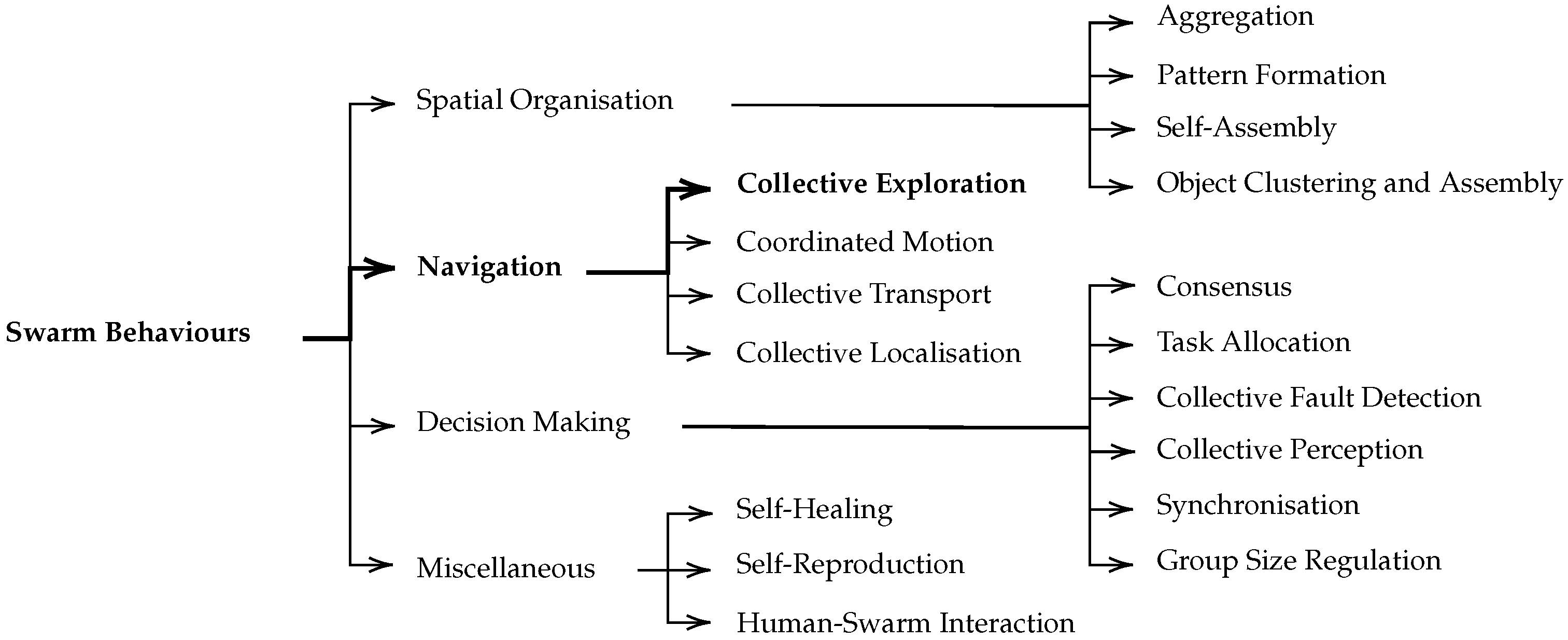
Such behaviours have been classified by Brambilla et al. [5], Schranz et al. [6] in four categories as depicted in Figure 1: spatial organisation (robots have to organise themselves to form patterns or simply aggregate), navigation (robots have to coordinate their movement), decision making (robots have to influence themselves to take a common decision) and miscellaneous (other significant behaviours which could not belong to any of the three previous categories). Since this work focusses on the area coverage by a swarm of UAVs, it falls in the “navigation” category containing four subcategories: collective exploration, coordinated motion, collective transport and collective localisation. The remainder of this section focusses on collective exploration, as it is the target of this work.

2.1. Manual Design of Robot/UAV Swarms

The literature contains a variety of studies based on path planning to manually design the behaviour of robots or UAVs, including in the context of coverage as surveyed in Cabreira et al. [7]. The idea is to compute the optimal path of robots/UAVs offline, i.e., before starting the mission. In some works, these precomputed paths may be updated or recomputed. For example, Siemiatkowska and Stecz [8] recalculates Vehicle Routing Planning (VRP) when UAVs detect a threat on their way. Additionally, the problem of path planning is often formulated as a variant of VRP. It is also the case of Semiz and Polat [9] who solves a problem of area coverage (differently from the problem tackled in this work). These path planning techniques are not comparable to the work proposed in this article. Indeed, most of these studies do not fit the above definition of a swarm. Nevertheless, with path planning techniques, UAVs follow the path calculated beforehand, which implies strong control from a human operator. Moreover, these techniques are usually exact methods and/or metaheuristics that are too expensive for online usage.

Another way to manually design robot/UAV swarms considers online techniques based on direct or indirect communication between robots/UAVs. Some of those are based on line-of-sight communication. The work of Nouyan et al. [10] consists in chaining a swarm of robots between two points where the robots have different colours according to the direction of the chain. Ducatelle et al. [11] propose a communication system for making a swarm of robots reach an unknown target point. However, when dealing with collective exploration, the vast majority relies on a stigmergy process such as pheromone-based systems. Some work focus on the design of the swarm system [12,13], which abstracts from the application, i.e., the collective task. The idea is to design a pheromone system as close as possible to how pheromones would evolve in nature. These pheromone systems are used to investigate the impact of using multiple pheromones in the context of a collective task [14,15].

Most of the literature, meanwhile, deals with task-specific systems, i.e., how to use the pheromone for the desired collective task. Kuiper and Nadjm-Tehrani [16] first introduced a pheromone-based system to optimise the coverage of an area by a swarm of UAVs. In that work, UAVs have to choose a direction according to the amount of repulsive pheromones left by other UAVs. Rosalie et al. [17] proposed an extension of the latter work where the random aspect is replaced by a chaotic system. The objective is to obtain a movement that seems unpredictable from the outside while being deterministic. Danoy et al. [18] combined the work of Kuiper and Nadjm-Tehrani [16] with a multi-hop clustering approach to consider the connectivity of the swarm during the coverage task. The added connectivity objective aims to maintain a good exchange of information within the swarm and, thus, improve its performance. Brust et al. [19] extended the previous work with a dual-pheromone model to tackle three objectives of the swarm: area coverage, swarm connectivity and target tracking.

Although such pheromone-based approaches have shown good results, Hunt et al. [20] show that they face limitations, particularly when the density of the swarm is very high (the number of robots/UAVs relative to the size of the area). Added to this limitation, such a pheromone-based behaviour has to be designed manually, which can be very time-consuming and specific to an application. For instance, the pheromone evaporation rate or the balance between different pheromones (in the case of using multiple types) may differ according to the emergent task of the swarm.

2.2. Automated Design of Robot/UAV Swarms

An approach that has recently raised some interest consists in automating the design of swarming behaviours, as mentioned by Birattari et al. [1]. This process can be assimilated to a hyper-heuristic which has been deeply surveyed by Burke et al. [21], Epitropakis and Burke [22], Burke et al. [23]. Hyper-heuristics are used more generally in optimisation for automating the design of heuristics for a given problem. Li and Malik [24] first assimilate that process to learning to optimise where they view an optimisation algorithm as a policy in a Markov Decision Process (MDP). In the context of robot/UAV swarms, a heuristic corresponds to the local behaviour of each UAV used to tackle global problems like optimising the coverage of an area.

2.2.1. Selective Approaches

Hyper-heuristics were first defined by Cowling et al. [25] as “heuristics to choose heuristics”. Their purpose was to select the best heuristic, among a set of predefined low-level heuristics, according to a given problem instance, which is referred to as selective hyper-heuristics. A high-level learning process, e.g., genetic programming, reinforcement learning or classifier, is then used for selection purposes. This process has only recently been applied in the context of the UAV / robot swarm and is still an open research area, as outlined by Birattari et al. [1]. The latter manifesto presents the current challenges of “automatically designing a swarm for any mission with a given class”. Most existing techniques consist in providing UAVs/robots with a set of predefined actions so that they can learn at each step which action to use according to the given task and the state of the environment. For instance, Birattari et al. [26] developed AutoMoDe, which is a framework to automate the design of a robot swarm with different specialisations (corresponding to each set of behaviours). Ligot et al. [27] extend the latter work with a way to automatically generate different missions along with a performance indicator. Reinforcement Learning (RL) is mainly used as a high-level algorithm. The idea is to represent the actions of RL by the different behaviours of the swarm. Yu et al. [28] used it in the context of a self-assembling swarm and Yu et al. [29] in the more specific case of surface cleaning. It is also used by Nagavalli et al. [30] to choose a sequence of behaviours for a given task, such as navigating in an environment with obstacles. These selective approaches are prominently used in the context of robot/UAV swarming as it is convenient to provide specific behaviours to a robot or UAV.

2.2.2. Generative Approaches

A second and more recent branch of hyper-heuristics relying on a generative approach exists in the literature but it has not received much attention yet in the robot/UAV community. Generative hyper-heuristics do not need a set of predefined low-level heuristics but a set of “building blocks” from which the high-level algorithm will construct possibly unseen low-level heuristics. This research direction was first mentioned by Duflo et al. [31,32] where the task of the swarm is represented as a multi-objective optimisation problem. RL is then used to generate distributed heuristics for this problem. A drawback of these methods is their tendency to favour one objective during the learning process. This work proposes to improve the state-of-the-art thanks to a more accurate description of the multi-objective optimisation problem and a novel hyper-heuristic for generating distributed heuristics for such a multi-objective problem.

3. CCUS3O Model

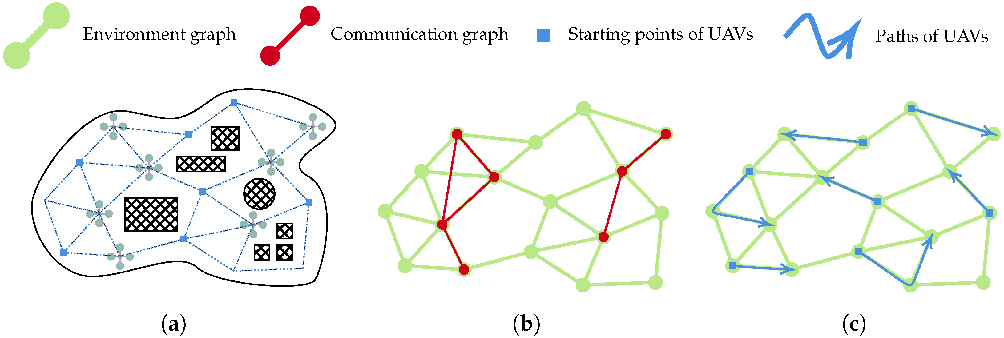
The following UAV swarm surveillance scenario is considered in this work: several UAVs equipped with ad hoc communication capabilities take off from different bases to cover a common area (see Figure 2a with blue squares as bases of UAVs). These UAVs evolve as a swarm that needs to cover as much area as possible, as fast as possible, while remaining as connected as possible. This connectivity aspect is crucial in such a distributed system, as it will enhance communication within the swarm. The local information of each UAV will, therefore, spread faster, which in turn will result in improved performance of the global system (i.e., swarm). In this context, the information exchanged by UAVs is the current solution according to their distributed knowledge. A formalisation of a solution is described in Section 3.1.4. Once the UAVs have finished covering the area, they must return to their base (i.e., initial starting point). Such a surveillance scenario can find numerous civil applications that require a fast and efficient coverage of a large area, such as search and rescue missions, forest fire or pollution detection.

Duflo et al. [31,32] designed the Coverage of a Connected-UAV Swarm (CCUS) optimisation problem for that purpose. It optimises the coverage of an area by a swarm of UAVs with two objectives: coverage speed and swarm connectivity. This work proposes to extend CCUS to a three-objective model, referred to as CCUS3O, which targets coverage time, coverage rate and connectivity. What motivates the introduction of a third objective is that the coverage objective in CCUS includes both the coverage time and the coverage rate in one single value. Such a scalarisation introduces a bias that not only can negatively impact the performance, but also reduces the explainability of the objective value. Using three objectives in CCUS3O, thus, permits us to have more atomic objectives. The remainder of this section first presents a formal definition of instances and solutions (see Section 3.1), followed by the evaluation of solutions according to the three objectives (see Section 3.2).

3.1. Formal Expression

The CCUS3O model considers two entities: an environment graph which is a discretisation of the area, and the communication graph, which depicts the communication network of the swarm. Both are represented in Figure 2b and detailed hereinafter.

3.1.1. Environment Graph

The environment graph is a discretisation of the environment that defines where UAVs can move and which ways they can take (see Figure 2b). It is represented as $G^e=\left(V,E^e\right)$ with V the set of vertices and $E^e$ the set of edges. This graph is here considered static, i.e., the set of edges remains the same along with their length and connected.

As a notation, $dist:V^2\to \mathbb{R}$ returns the length of the shortest path between two given vertices. The neighbourhood of a vertex v is represented by ${\mathcal{N}}^e\left(v\right)$, which is the set of every vertex linked to v in the environment graph.

3.1.2. Communication Graph

The communication graph indicates the position of UAVs (i.e., vertices) and connects them (i.e., edges) if they are close enough for communicating, i.e., below a predefined communication range threshold $D^{\mathit{com}}$ from each other (see Figure 2b). The value of $D^{\mathit{com}}$ is directly related to the ad hoc communication setup. The communication graph is noted $G^c=\left(U,E^c\right)$, with U the set of UAVs. Unlike the environment graph, it is dynamic and not always connected, since the position of UAVs changes during the coverage task.

As a notation, $pos:U\to V$ returns the position of a given UAV, i.e., the vertex on which the UAV is currently located. Moreover, the neighbourhood of a UAV u is depicted by ${\mathcal{N}}^c\left(u\right)$, which is the set of all UAVs in the communication range of u.

3.1.3. Definition of Instances

A CCUS3O instance is defined by an environment graph and an initial communication graph and can be written as $I=\left(G^e,G^c\right)$. Since $G^c$ belongs to the instance, the initial position of UAVs is, therefore, specific, which means that two different initial positions result in two different instances. The set of CCUS3O instances is depicted as $\mathbb{I}$. Given two graphs $G^e=\left(V,E^e\right)$ and $G^c=\left(U,E^c\right)$, then $I=\left(G^e,G^c\right)\in \mathbb{I}$ if and only if $\forall u\in U$

$${\mathcal{N}}^c\left(u\right)=\left\{u^{\prime }\in U\backslash \left\{u\right\}\mid dist(pos\left(u\right),pos\left(u^{\prime }\right)\le D_{\mathit{com}}\right\}$$

From this definition, an instance class can be defined by an environment graph and the size of the communication graph. Given a connected graph G and an integer $k>0$, the class of instances $\mathcal{C}(G,k)$, thus, represents the instances with k UAVs in an environment graph G. Thus, instances of the same class only differ in terms of the initial position of UAVs.

$$\mathcal{C}(G,k)=\left\{\left(G,\left(U,E^c\right)\right)\in \mathbb{I}\mid \left|U\right|=k\right\}$$

3.1.4. Definition of Solutions

A solution for a CCUS3O instance $I\in \mathbb{I}$ is a set of paths in $G^e$. It can be defined as $S={\left\{P_u\right\}}_{u\in U}$, with each path $P_u$ starting at the origin vertex of the corresponding UAV u, as represented in Figure 2c. In addition, a solution is considered feasible if and only if the paths $P_u$ are cycles, i.e., $P_u\left[1\right]=P_u\left[\left|P_u\right|\right]$, $\forall u\in U$. In the CCUS3O scenario, it means that every UAV has returned to its starting point. As a notation, $\overline{S}$ refers to the vertices of $G^e$ not appearing in S, i.e., not visited by any UAV.

$$\overline{S}=\left\{v\in V\mid \nexists u\in U,v\in P_u\right\}$$

3.2. Objective Values

At any moment during the execution of the coverage mission, the current solution can be evaluated according to the three CCUS3O objectives: coverage time, coverage rate and connectivity. Any solution S is, thus, evaluated by $O\left(S\right)\in {\mathbb{R}}^3$:

$$O\left(S\right)=\left(\begin{array}{c}{O}^{\left(\mathit{rate}\right)}\left(S\right)\\ O^{\left(\mathit{time}\right)}\left(S\right)\\ O^{\left(\mathit{conn}\right)}\left(S\right)\end{array}\right)$$

where $O^{\left(\mathit{rate}\right)}\left(S\right)$, $O^{\left(\mathit{time}\right)}\left(S\right)$ and $O^{\left(\mathit{conn}\right)}\left(S\right)$ refer to the objective values of S according to the coverage time, the coverage rate and the connectivity. Let $\mathcal{O}=\left\{\mathit{rate},\mathit{time},\mathit{conn}\right\}$ denote the set of CCUS3O objectives.

3.2.1. Coverage Rate

During a coverage mission, UAVs are expected to cover as much area as possible. In CCUS3O, it corresponds to maximising the number of vertices visited in the environment graph. For any solution S, its objective value for the coverage rate $O^{\left(\mathit{rate}\right)}\left(S\right)$ is then defined as the difference between the number of non-visited vertices, i.e., $\left|\overline{S}\right|$, and the number of vertices in the environment graph, i.e., $\left|V\right|$.

$$O^{\left(\mathit{rate}\right)}\left(S\right)=\left|\overline{S}\right|-\left|V\right|$$

The result is always a nonpositive number to obtain a minimisation objective. For missions where the whole area covered is considered, this objective is then equal to the opposite of the number of vertices in the environment graph.

3.2.2. Coverage Time

In addition to covering as much area as possible, the time for the UAVs to return to their base must be minimised. In the CCUS3O model, UAVs are considered to fly at a constant speed. The fact that the speed is constant shows that the time spent and the distance travelled are proportional, regardless of the value of the speed. Therefore, the coverage time can be calculated from the distance travelled by the UAVs. During a coverage mission, the UAVs do not return to their base at the same moment. Therefore, the total coverage time corresponds to the time needed by the UAV that finished last, that is, with the longest trip. For any solution S (including nonfeasible ones), $O^{\left(\mathit{time}\right)}\left(S\right)$ is defined as:

$$O^{\left(\mathit{time}\right)}\left(S\right)=\underset{u\in U}{max}{l}_u$$

where $l_u$ is the length of the path made by UAV u at the current time and the path from the current position to the starting vertex (i.e., base station). Thus, it represents the length of the cycle made by the UAV u if the latter comes back to its initial vertex from the current position.

$$l_u=\underset{\mathrm{distance}\mathrm{from}\mathrm{the}\mathrm{initial}\mathrm{vertex}}{\underbrace{\phantom{{\sum }_{i=1}}dist\left(pos\left(u\right),P_u\left[1\right]\right)}}+\underset{\mathrm{distance}\mathrm{travelled}\mathrm{so}\mathrm{far}}{\underbrace{\sum _{i=1}^{\left|P_u\right|-1}dist\left(P_u\left[i\right],P_u[i+1]\right)}}$$

Since the objective is to cover the area as fast as possible, the coverage time objective should be minimised. Furthermore, minimising the longest cycle (compared to minimising the average, for instance) prevents the situation where some UAVs finish their tour much earlier than the other ones.

3.2.3. Connectivity

Efficient information sharing is of prime importance for UAV swarms, which are highly mobile ad hoc networks relying on distributed decision making. In CCUS3O, it is considered that every UAV u asynchronously shares its local information with every UAV in its communication neighbourhood depicted by ${\mathcal{N}}^c\left(u\right)$. As a consequence, every UAV in the same connected component of the communication graph has similar local information about the area that has been covered. Therefore, this connectivity objective aims at minimising the average number of connected components in $G^c$. For this purpose, a discretisation of time $T=\left\{t_1,t_2,\cdots \right\}\subset \mathbb{R}$ is considered, and for a solution S, $T_S\subset T$ contains every time lower than or equal to the current time of S. The objective value for the connectivity $O^{\left(\mathit{conn}\right)}\left(S\right)$ is then obtained as:

$$O^{\left(\mathit{conn}\right)}\left(S\right)=\frac{1}{\left|T_S\right|}\sum _{t\in T_S}{c}_t$$

where $c_t$ is the number of connected components in $G^c$ at time t.

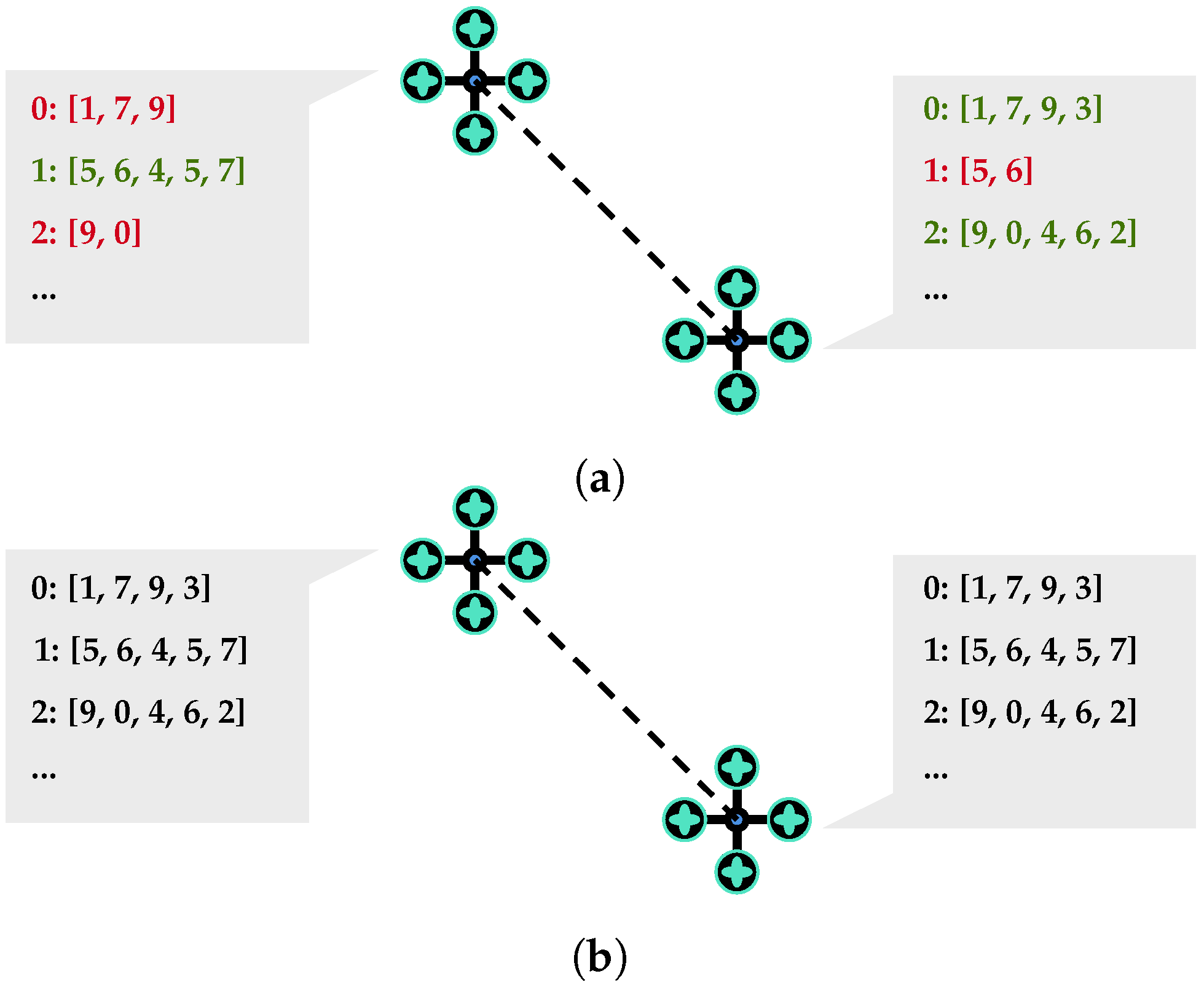
Each UAV keeps in memory the representation of the solution (based on its distributed knowledge), i.e., the path made by each UAV so far. When two UAVs communicate, they share that information and keep for each path the most recent one, as shown in Figure 3.

4. Proposed QLHH-II Algorithm

The purpose of QLHH-II is to generate, using Q-learning, the CCUS3O heuristic that will be used by each UAV. This section first presents the structure of the proposed generative hyper-heuristic QLHH-II. It then details every step of the algorithm. Finally, it describes its general pseudocode. Since QLHH-II extends QLHH designed by Duflo et al. [31], the improvement of the model is explained in Section 4.1.2 and a comparison of the heuristics generated by both models is made in Section 6.2.

4.1. Hyper-Heuristic Structure

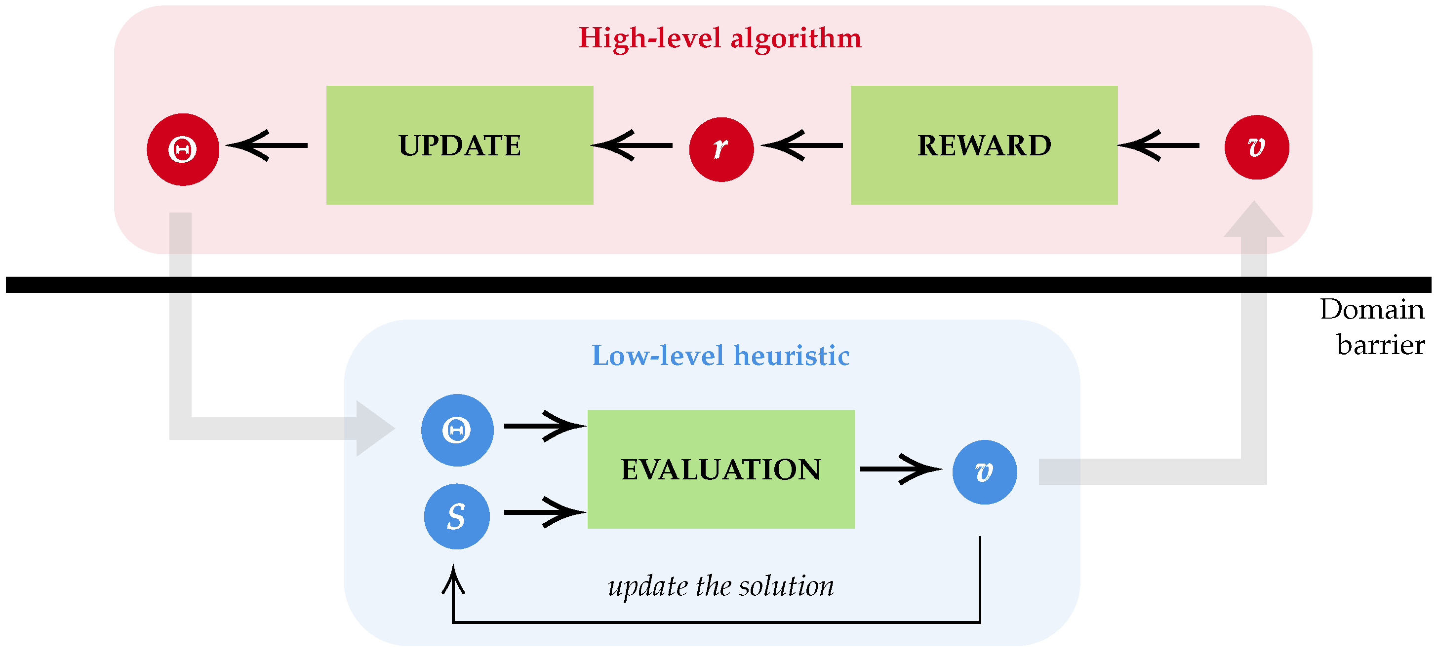
A hyper-heuristic consists of a high-level algorithm performing a search process in a space of low-level heuristics. These two levels depict the concept of learning to optimise with the high-level algorithm as the learning part and the low-level heuristic as the optimisation part. In this work, the low-level space is composed of CCUS3O heuristics, while the high-level algorithm is QL. More precisely, all CCUS3O heuristics are based on one heuristic template (see Algorithm 1). From that template is extracted a dynamic component which corresponds to the search space for the high-level algorithm (see Section 4.1.2).

The high-level/low-level structure is illustrated in Figure 4 (detailed in Section 4.2). The barrier domain shows the separation between the low-level heuristics, which depend on the problem, and the high-level algorithm, which is problem independent.

Algorithm 1: Low-level heuristic template

4.1.1. Low-Level Heuristics

In the context of this work, UAVs are moving as a swarm in a distributed way. The generated low-level heuristic should thus be distributed. Each UAV asynchronously has the same behaviour as described in Algorithm 1. At each step, every UAV u evaluates the vertices of the environment graph with a scoring function $f_u$ and chooses to fly to the one maximising that function (line 4). If the chosen vertex is not in the neighbourhood of the current one, i.e., $v_{\mathit{next}}\notin {\mathcal{N}}^e\left(pos\left(u\right)\right)$, then the UAV simply uses the shortest path between both vertices to reach the destination (line 5). When every vertex has been covered by UAVs, they fly back to their initial position (line 7). Since the low-level heuristics are distributed, the latter condition may not be correct. Each UAV indeed takes this decision based on its local knowledge. This means that one or more UAVs may keep flying while the environment graph is actually fully covered.

The low-level heuristic template depicted in Algorithm 1 thus describes the search space when every low-level heuristic is represented by its scoring function $f_u$. For example, if $f_u\left(v\right)=-dist(pos\left(u\right),v)$, the UAVs will then fly to the nearest vertex. Such a behaviour thus belongs to the space of low-level heuristics.

4.1.2. High-Level Algorithm

The goal of the high-level algorithm is to find the best definition of the scoring function $f_u$. A QL algorithm is used for this purpose since the function $f_u$ can be assimilated into a state action value function, as detailed below.

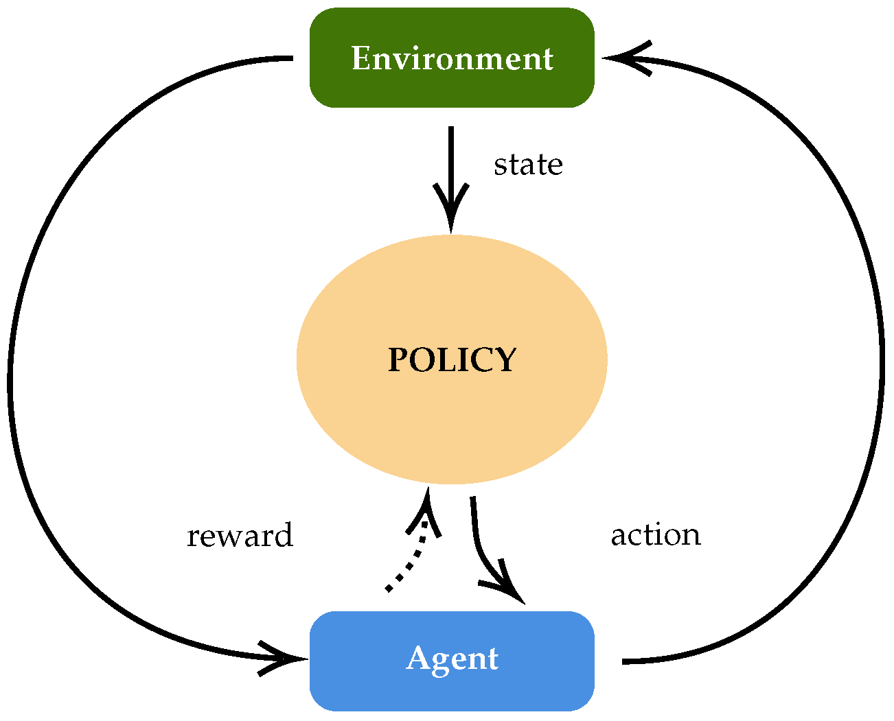
The idea of RL, as depicted in Figure 5, is to make an agent evolve in an environment. The policy of the agent makes him choose an action according to the current state of the environment. This action then produces a reward that the agent uses to modify its policy so that the next choices of action are expected to be better. QL works with a function Q that is a state action value function. This means that Q evaluates an action from a given state. Therefore, the policy consists of choosing the action to maximise Q at a certain state. The purpose of QL is then to learn the Q function so that $Q(s,a)$ represents the maximal reward obtainable by choosing the action a from the state s.

With function $f_u$ as a state-action value function, there is still the need to map the components of the CCUS3O context into RL components, i.e., to define the states and actions. Here is the mapping that is used in QLHH-II: UAVs are RL agents; the current state of the environment in RL is considered here as the current solution; an action is assimilated to a vertex from the environment graph as the next destination of a UAV. Consequently, finding the next vertex to go, given the current solution, corresponds to the RL policy, which makes an agent choose an action from a certain state. Considering that, the line 4 in Algorithm 1 is equivalent to a QL policy with $f_u$ as the state-action value function, i.e., the Q function.

Using QL here comes with two main challenges based on the nature of CCUS3O. The first one is to use RL in a multi-agent context, which is referred to as Multi-Agent Reinforcement Learning (MARL). The model used here is the most basic one, with full cooperation and all of the agents sharing the same policy. Secondly, RL is here used to generate heuristics for a multi-objective problem. The area of Multi-Objective Reinforcement Learning (MORL) has shown a growing interest in the past few years, but it still lacks existing techniques and benchmarks. Most of the literature considers scalarisation techniques (i.e., reducing a multi-objective policy into a single one) [33]. That process is used differently in QLHH-II than in the original QLHH. QLHH indeed provides multiple policies that are scalarised into a single one, while QLHH-II uses a single policy and scalarises the multiple rewards into a single one. The multiple policies of QLHH have their own learning process from their own reward. This independence between objectives has shown difficulty in balancing them in the generated heuristic, which is an issue in itself. If it turns out that connectivity has more emphasis, UAVs are flying together rather than visiting new vertices, which can make episodes very long in the context of CCUS(3O) since the terminal condition for UAVs to return to their base is that every vertex is visited. To overcome this issue, the idea with QLHH is to update the weights during the scalarisation according to objectives “needing support” but it obliges the user to define higher and lower bounds for each objective, which can be time consuming. The single policy of QLHH-II is intended to break this independence and improve the balance of objectives in the generated heuristics.

4.2. QLHH-II Detailed Steps

This section details the three steps of QLHH-II shown in Figure 4: (1) the evaluation of the vertices by the UAVs to choose the next destination, (2) the computation of the reward for such a choice of action and (3) the update of the policy according to the obtained rewards. The policy used here is parameterised by $\mathsf{\Theta }$. It means that the entire QLHH-II process consists of learning the value of $\mathsf{\Theta }$, which defines the generated heuristic.

4.2.1. Evaluation

Each UAV uses the Q function from QL to evaluate a vertex, i.e., an action, at the current solution, i.e., the state. Therefore, the function $Q_u(S,v)$ gives a score for the UAV u to fly to vertex v at solution S. The choice of action for the UAV u, therefore, consists of choosing the vertex that maximises $Q_u$.

Embedding Structure

The purpose of the following embedding structure is to represent a vertex v, according to the knowledge of a UAV u, by a p-dimensional vector ${\mu }_{uv}$.

$${\mu }_{uv}=\mathtt{relu}\left({\theta }_1·x_{uv}\right)\in {\mathbb{R}}^p$$

with ${\theta }_1\in {\mathbb{R}}^{p\times 3}$ and relu is the rectified linear unit; where $x_{uv}\in {\mathbb{R}}^3$ is the vector of state variables of vertex v for UAV u. Each component of that vector corresponds to one CCUS3O objective. For the coverage time, it equals 1 if the vertex is on the shortest path from the position of the UAV u and its initial position, and 0 otherwise. For the coverage rate, it equals 1 if the vertex has been visited by any UAV and 0 otherwise. For the connectivity, it equals 1 if the vertex is in the communication range of another UAV and 0 otherwise. The formal definition is given below.

$$\begin{array}{cc}\hfill x_{uv}^{\left(\mathit{time}\right)}& =\left\{\begin{array}{cc}1\hfill & \mathrm{if}dist(pos\left(u\right),P_u\left[1\right])=dist(pos\left(u\right),v)+dist(v,P_u\left[1\right])\hfill \\ 0\hfill & \mathrm{otherwise}\hfill \end{array}\right.\hfill \\ \hfill x_{uv}^{\left(\mathit{rate}\right)}& =\left\{\begin{array}{cc}1\hfill & \mathrm{if}v\notin \overline{S}\hfill \\ 0\hfill & \mathrm{otherwise}\hfill \end{array}\right.\hfill \\ \hfill x_{uv}^{\left(\mathit{conn}\right)}& =\left\{\begin{array}{cc}1\hfill & \mathrm{if}\exists u^{\prime }\in U\backslash \left\{u\right\},dist(pos\left(u^{\prime }\right),v)\le D^{\mathit{com}}\hfill \\ 0\hfill & \mathrm{otherwise}\hfill \end{array}\right.\hfill \end{array}$$

Parameterisation

The scoring function $Q_u\left(S,v;\mathsf{\Theta }\right)$ is a matrix computation that takes as input two p-dimensional vectors, one for the current solution and one for a vertex to evaluate. For a UAV u, a vertex v is directly represented by ${\mu }_{uv}$ while the solution is represented by the sum over every vertex, i.e., ${\sum }_{v\in V}{\mu }_{uv}$.

$$Q_u\left(S,v;\mathsf{\Theta }\right)={\theta }_2^{\top }·\mathtt{relu}\left(\left[{\theta }_3·\sum _{v\in V}{\mu }_{uv},{\theta }_4·{\mu }_{uv}\right]\right)$$

with ${\theta }_2\in {\mathbb{R}}^{2p}$ and ${\theta }_3,{\theta }_4\in {\mathbb{R}}^{p\times p}$; where $[·,·]$ is the concatenation operator.

Due to the embedding structure described above, a state and an action (respectively a solution and a node) are represented by two p-dimensional vectors ${\sum }_{v\in V}{\mu }_{uv}$ and ${\mu }_{uv}$, respectively. The policy of the high-level Q-learning algorithm can, thus, be used on different instances of different size (not the same number of nodes in the environment graph nor the same number of UAVs). This makes it possible to learn the policy on different instances and to apply the generated heuristic to unknown environments.

4.2.2. Reward

In RL, the reward is given for an action chosen in a certain state, i.e., for a vertex chosen in a certain solution in the CCUS3O context. Let $S_t$ be the current solution at the time t, $v_t$ the vertex is chosen by a UAV at that time and $S_{t+1}$ the resulting solution, the reward for such an action is given by

$$r\left(S_t,v_t\right)=O\left(S_t\right)-O\left(S_{t+1}\right)\in {\mathbb{R}}^3$$

Since the CCUS3O objectives must be minimised, the reward must be positive if the objective value after the action is smaller than before and vice versa. The reward is, therefore, $O\left(S_t\right)-O\left(S_{t+1}\right)$ instead of $O\left(S_{t+1}\right)-O\left(S_t\right)$. Therefore, minimising objectives is equivalent to maximising the reward.

Cumulative Reward

In QLHH-II, an update of the policy is made for a frame of $\tau$ movements. Therefore, it considers a cumulative reward, i.e., the sum of consecutive rewards. The cumulative reward of $\tau$ iterations from time t is given by $R_{t,\tau }$. Due to the above definition of the reward calculated for an action, $R_{t,\tau }$ is equivalent to the difference in the objective value of the solutions before and after the $\tau$ movements, i.e., $S_t$ and $S_{t+\tau }$, respectively.

$$R_{t,\tau }=\sum _{i=0}^{\tau -1}r\left(S_{t+i},v_{t+i}\right)=O\left(S_t\right)-O\left(S_{t+\tau }\right)\in {\mathbb{R}}^3$$

Scalarisation

The vector of cumulative rewards $R_{t,t+\tau }$, i.e., for a frame of $\tau$ movements from time t, is reduced to a scalar reward $r_t$ using a linear scalarisation consisting of a convex combination of every reward.

$$r_t=\sum _{o\in \mathcal{O}}{w}^{\left(o\right)}·R_{t,\tau }^{\left(o\right)}\in \mathbb{R}$$

with ${\sum }_{o\in \mathcal{O}}{w}^{\left(o\right)}=1$. For experiments described later, all objectives are given the same importance, i.e., $w^{\left(\mathit{rate}\right)}=w^{\left(\mathit{time}\right)}=w^{\left(\mathit{conn}\right)}=\frac{1}{3}$.

4.2.3. Update

For each action made, the following tuple is stored in memory $\mathcal{M}$: UAV performing the action; state in which the action is made; action considered; the cumulative reward of the $\tau$ following actions; state after these $\tau$ actions. In CCUS3O, at each time step t, the tuple $\left(u,S_{t-\tau },v_{t-\tau },r_{t-\tau },S_t\right)$ is thus added in $\mathcal{M}$. 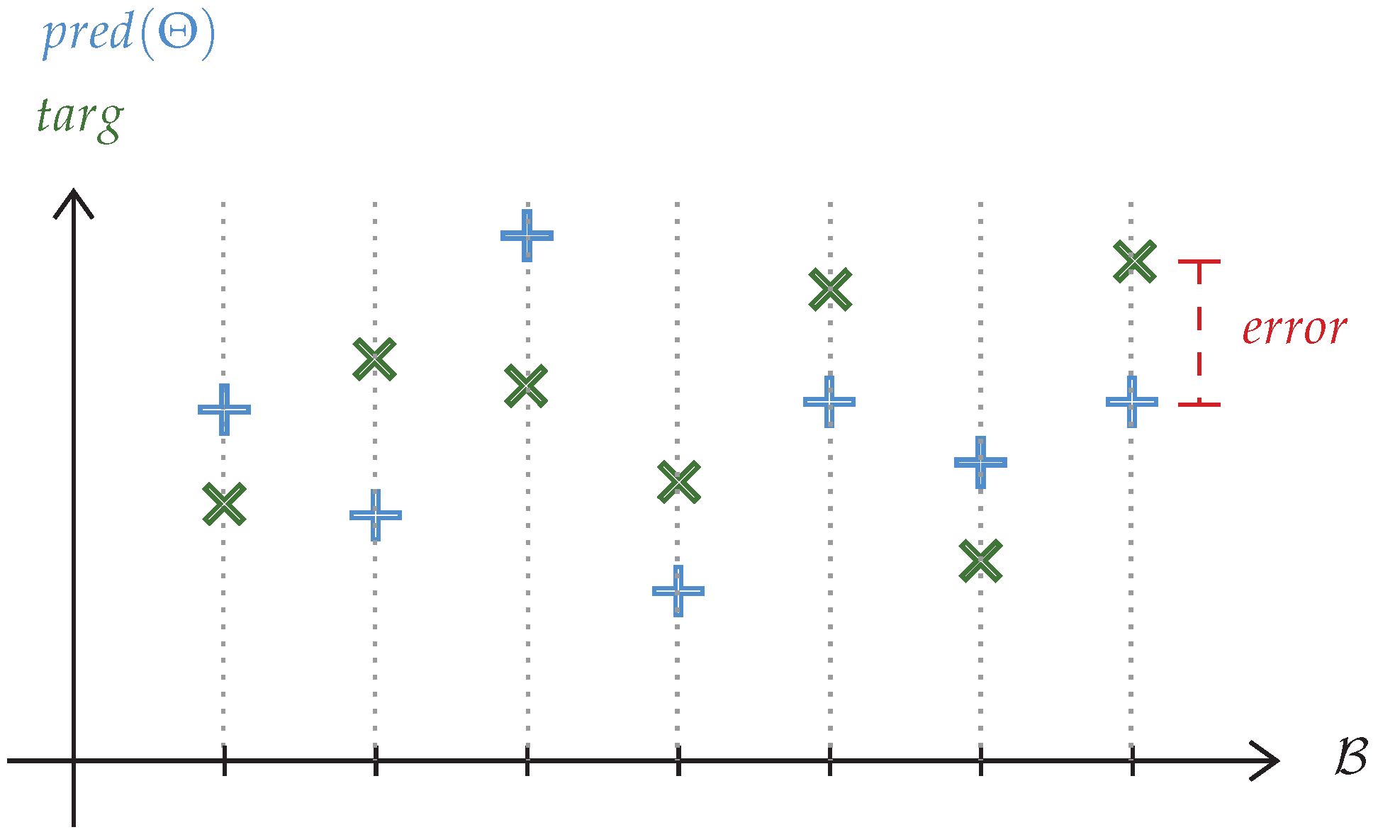Every such item $i=\left(u^{\left(i\right)},S^{\left(i\right)},v^{\left(i\right)},r^{\left(i\right)},S^{\prime \left(i\right)}\right)\in \mathcal{M}$ makes it possible to compute the following two values depicted in Figure 6:

$$\begin{array}{cc}\hfill & {\mathit{pred}}_i\left(\mathsf{\Theta }\right)=Q_{u^{\left(i\right)}}\left(S^{\left(i\right)},v^{\left(i\right)};\mathsf{\Theta }\right)\hfill \\ \hfill & {\mathit{targ}}_i=r^{\left(i\right)}+\gamma ·\underset{v\in V}{max}{Q}_{u^{\left(i\right)}}\left(S^{\prime \left(i\right)},v;\mathsf{\Theta }\right)\hfill \end{array}$$

with $\gamma \in [0,1]$ the discount factor; ${pred}_i\left(\mathsf{\Theta }\right)$ the value of the evaluation obtained by choosing $v^{\left(i\right)}$ from $S^{\left(i\right)}$ with the current $\mathsf{\Theta }$, and ${\mathit{targ}}_i$ the value of the target evaluation, i.e., the evaluation that should have been made according to the obtained reward and future reward. After every movement of a UAV, $\mathsf{\Theta }$ is, thus, updated by processing a Stochastic Gradient Descent (SGD) step for a mini-batch $\mathcal{B}\subset \mathcal{M}$ randomly selected from the memory to minimise the loss, formally defined below, being the squared mean error.

$$\mathit{loss}=\sum _{i\in \mathcal{B}}{\left({\mathit{pred}}_i\left(\mathsf{\Theta }\right)-{\mathit{targ}}_i\right)}^2$$

It should be noted that the target value $\mathit{targ}$ is considered a constant. It means that during its calculation, there is no trace of the variable $\mathsf{\Theta }$ for the SGD, unlike the predicted value, which depends on $\mathsf{\Theta }$.

4.3. General Pseudo-Code

Algorithm 2 describes the whole process of the proposed QLHH-II. Firstly, $\mathsf{\Theta }$ is randomly initialised (line 3). Then an epoch consists of tackling every instance of $\mathcal{I}$. For example, every UAV has the same process asynchronously. As long as there are still unvisited vertices according to their knowledge (line 9), they choose a new destination according to the evaluation $Q_u$ function (line 11, see Section 4.2.1). With a certain probability depending on the exploration rate $ϵ\in [0,1]$, the choice of the new destination is made uniformly at random among every vertex instead. The UAVs then use the shortest path to go to their chosen vertex (line 12). After the movement is completed, the reward can be computed (line 13, see Section 4.2.2). If at least $\tau$ movements have been performed, the memory and $\mathsf{\Theta }$ are updated (lines 15–16, see Section 4.2.3). Lines 21–24 simply correspond to the action of a UAV to fly back to its initial position. It should be noted that for that last action, the final solution is not added to the memory tuple, since it corresponds to a terminal state and is therefore not used in the computation of the targeted evaluation. Finally, $\mathsf{\Theta }$ returns after the last epoch, which represents the returned low-level heuristic.

Algorithm 2: Pseudo-code of QLHH-II

5. Experimental Setup

This section introduces the setup used to conduct the experiments. In the following, the metrics used to assess the performance of the generated heuristic with QLHH are presented. Then, the manually designed heuristic used as the basis of comparison is introduced. Finally, details on the whole experimental process are provided.

5.1. Performance Metrics

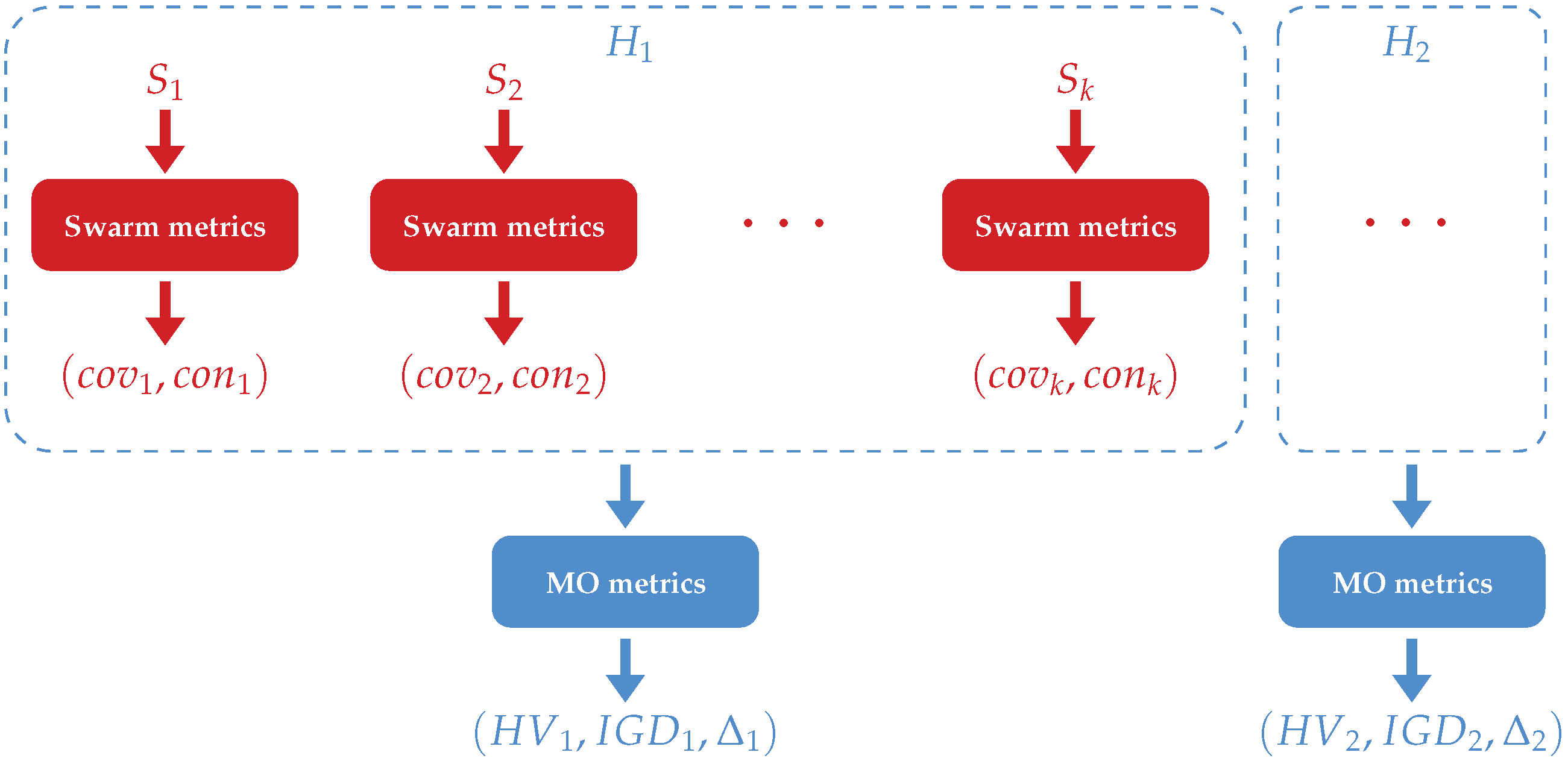
Two types of metrics are presented in this section: the metrics used to evaluate the performance of a swarm according to the coverage and the connectivity; the metrics used for comparing two sets of non-dominated solutions in multi-objective optimisation. As depicted in Figure 7, a heuristic $H_1$ provides different solutions $S_1,S_2,\cdots ,S_k$. The swarm metrics evaluate these solutions according to coverage and connectivity. For a solution $S_i$, a couple of values $({\mathit{cov}}_i,{\mathit{con}}_i)$ is, therefore, returned and can be displayed in a two-dimensional coordinate system. Therefore, the obtained set of 2D points represents the heuristic $H_1$, whose performance can finally be evaluated using the three MO metrics.

5.1.1. Swarm Metrics

Here, two state-of-the-art metrics [19] are defined to assess the performance of the swarm. The coverage speed evaluates the quality of coverage, while the number of connected components evaluates the connectivity.

Coverage Speed

Let $n_v^{\left(t\right)}$ be the number of times the vertex $v\in V$ has been visited at the time step $t\in \{0,\cdots ,T\}$. Then, $\mathtt{speed}\left(r\right)$ is the time required by the swarm to cover the rate $r\in [0,1]$ of the environment graph.

$$\mathtt{speed}\left(r\right)=\underset{0\le t\le T}{arg\; min}\left\{\frac{\left|\left\{v\in V\mid n_v^{\left(t\right)}>0\right\}\right|}{\left|V\right|}\ge r\right\}$$

Number of Connected Components

This metric is similar to the definition of the connectivity objective of CCUS. The value of number is then the average number of connected components in the communication graph.

$$\mathtt{number}=O^{\left(\mathit{conn}\right)}\left(S_T\right)$$

5.1.2. Multi-Objective Metrics

To evaluate the quality of CCUS solutions, three metrics considering the multi-objective aspect have been used: the Hyper-Volume (HV), the Inverted Generational Distance (IGD) and the spread ($\Delta$). For a set of solutions, let $P={\left\{p_i\right\}}_i$ be the subset of non-dominated ones, and $P^{*}={\left\{p_i^{*}\right\}}_i$ be the optimal Pareto front. These two sets are ordered according to one of their objective values. The Euclidean distance in the objective space between two points from both fronts is given by $d:\left\{1,\cdots ,\left|P^{*}\right|\right\}\times \{1,\cdots ,\left|P\right|\}\to {\mathbb{R}}_{+}$.

$$d(i,j)={∥p_i^{*}-p_j∥}_2$$

Hyper-Volume (HV)

HV represents the volume in the objective space covered by the points in P, relative to a reference point w.

$$HV=\mathtt{volume}\left(\bigcup _{i=1}^{\left|P\right|}{v}_i\right)$$

with $v_i$ the hypercube in the objective space made by $p_i$ and w.

Inverted Generational Distance (IGD)

IGD measures the proximity of the front P to the optimal front $P^{*}$.

$$IGD=\frac{1}{\left|P^{*}\right|}\sqrt{\sum _{i=1}^{\left|P^{*}\right|}{\left(\underset{1\le j\le \left|P\right|}{min}d(i,j)\right)}^2}$$

Spread (Δ)

$\Delta$ indicates how well the non-dominated solution are spread on the front P. It also takes into account the width of P compared to the optimal front $P^{*}$.

$$\Delta =\frac{d_f+d_l+{\displaystyle \sum _{i=1}^{\left|P\right|-1}}\left|d_i-\overline{d}\right|}{d_f+d_l+\left(\left|P\right|-1\right)\overline{d}}$$

with $d_f=d(1,1)$ and $d_l=d\left(\left|P^{*}\right|,\left|P\right|\right)$ the distances in the objective space between the first edges of P and $P^{*}$ and their last edge. Moreover, $d_i={∥p_i-p_{i+1}∥}_2$ is the distance between two adjacent points in P, with $\overline{d}=\frac{1}{\left|P\right|}{\sum }_{i=1}^{\left|P\right|-1}{d}_i$ the average distance.

5.2. Comparison Heuristics

To evaluate the performance of the heuristic generated by QLHH-II, it has been executed on different instances along with other heuristics which are presented in this section. The first heuristic has been designed manually to specifically tackle CCUS3O, while the two others are state-of-the-art pheromone-based heuristics that aim to cover an area.

5.2.1. Manually-Designed Heuristic

The Weighted Objective (WO) heuristic has been designed to tackle CCUS3O instances. It belongs to the space of low-level heuristics (defined in Algorithm 1), where the scoring function $f_u$ depends on three values (one per CCUS3O objective).

$$f_u\left(v\right)=\sum _{o\in \mathcal{O}}{a}_{uv}^{\left(o\right)}$$

with

$$\begin{array}{cc}{a}_{uv}^{\left(\mathit{time}\right)}\hfill & =W-dist(pos\left(u\right),v)-dist\left(v,P_u\left[0\right]\right)\hfill \\ a_{uv}^{\left(\mathit{rate}\right)}\hfill & =W·x_{uv}^{\left(\mathit{rate}\right)}\hfill \\ a_{uv}^{\left(\mathit{conn}\right)}\hfill & =min\left(W,W+D^{\mathit{com}}-\underset{u^{\prime }\in U\backslash \left\{u\right\}}{min}dist\left(v,pos\left(u^{\prime }\right)\right)\right)\hfill \end{array}$$

The value of W is set arbitrarily. For the coverage time objective, the weight linearly decreases according to the distance of the path from the current position to the initial position passing by the vertex to be evaluated. The weight of the coverage rate objective is equivalent to the state variable of the vertex to evaluate. For the connectivity objective, the weight depends on the distance to the closest UAV from the vertex to evaluate. If the latter distance is lower than $D^{\mathit{com}}$, i.e., is in the communication range of a UAV, then the weight is maximum; otherwise, it linearly decreases according to that distance. Even though the quality of WO is not guaranteed, it makes it possible to compare the performance of the heuristic generated by QLHH-II with behaviour more relevant than a random process.

5.2.2. Pheromone-Based Heuristics

As explained in Section 2, different techniques based on pheromone have been used in the context of area coverage by a swarm of robots/UAVs. Two have been implemented here to assess the quality of the coverage provided by the generated heuristic. For both heuristics, the behaviour is very similar to the one described in Algorithm 1. However, they do not belong to the space of low-level heuristic since the choice of the next position v for a UAV at a position $v_{\mathit{curr}}$ is stochastic and thus depends on a probability $\mathbb{P}\left(v\mid v_{\mathit{curr}}\right)$.

Heuristic Φ: The first heuristic, referred to as Φ, is based on repulsive pheromones [16], i.e., UAVs drop pheromones on their way to indicate visited places. The probability of a UAV going to a position is then inversely proportional to the amount of pheromones at that position (i.e., the more pheromones, the less chance). The environment in which UAVs are evolving is a grid, and at each iteration, UAVs assign the current coverage time to their current position. So each position is assigned a value that corresponds to the last time a UAV has visited it. As with repulsive pheromones, the lower the value assigned to a position, the higher the chance that UAVs have of choosing that position. Given a position v, let $t_v$ be the time assigned to that position and $\mathcal{N}\left(v\right)$ be the set of adjacent positions. The probability of going to a position v for a UAV at position $v_{\mathit{curr}}$ is

$$\mathbb{P}(v\mid v_{\mathit{curr}})=\left\{\begin{array}{cc}{\displaystyle \frac{T-t_v}{\left(\left|\mathcal{N}\left(v_{\mathit{curr}}\right)\right|-1\right)·T}}\hfill & \mathrm{if}v\in \mathcal{N}\left(v_{\mathit{curr}}\right)\hfill \\ 0\hfill & \mathrm{otherwise}\hfill \end{array}\right.$$

with $T={\displaystyle \sum _{v\in \mathcal{N}\left(v_{\mathit{curr}}\right)}}{t}_v$.

Heuristic Φ-K: The drawback of the heuristic Φ is that it does not consider the connectivity of the swarm. That is the purpose of the work, ref. [18] which adds a dynamic clustering algorithm, the so-called KHOPCA [34], to maintain connectivity within the swarm of UAVs. Let this heuristic be Φ-K. KHOPCA algorithm dynamically assigns a state value $s\left(u\right)$ to each UAV u that represents the distance to the cluster head ($s\left(u\right)=0$ if u is the cluster head). For a UAV u, let $\mathcal{N}\left(u\right)$ be the set of UAVs in the communication range of u. Then, $s\left(u\right)$ is iteratively updated by following four simple rules:

$$s\left(u\right)=\left\{\begin{array}{cc}\underset{u^{\prime }\in \mathcal{N}\left(u\right)}{min}s\left(u^{\prime }\right)+1\hfill & \mathrm{if}\underset{u^{\prime }\in \mathcal{N}\left(u\right)}{min}s\left(u^{\prime }\right)<s\left(u\right)\hfill \\ 0\hfill & \mathrm{if}\underset{u^{\prime }\in \mathcal{N}\left(u\right)}{min}s\left(u^{\prime }\right)=k\hfill \\ s\left(u\right)+1\hfill & \mathrm{if}s\left(u\right)\ne 0\wedge s\left(u\right)<\underset{u^{\prime }\in \mathcal{N}\left(u\right)}{min}s\left(u^{\prime }\right)\hfill \\ s\left(u\right)+1\hfill & \mathrm{if}s\left(u\right)=0\wedge \underset{u^{\prime }\in \mathcal{N}\left(u\right)}{min}s\left(u^{\prime }\right)=0\hfill \end{array}\right.$$

where $k+1$ is the number of UAVs (k is the biggest possible distance from the cluster head). At initialisation, $s\left(u\right)=k$ for every UAV u. At each iteration, UAVs which are not cluster heads follow their cluster with a certain probability PK, otherwise they choose their next position according to the probability defined in the heuristic Φ. When a UAV follows its cluster, it decides to go to the position of its neighbour (a UAV in its communication range) with the lowest state value. Since the value of PK has a high impact on the quality of the coverage, let Φ-K_PK denote this heuristic with a certain value for PK.

5.3. Experimental Process

For the experiments, all of the instances consider a grid graph as an environment graph. An instance class is then defined by its grid dimension and the number of UAVs in the swarm (see Section 3.1.3). The set of parameters present is presented in

Table 1. Experimental parameters used for training QLHH-II.

Parameter Name	Notation	Value
maximal distance of communication	$D^{\mathit{com}}$	4
exploration rate	$ϵ$	0.05
discount factor	$\gamma$	0.9
size of movement frame	$\tau$	10
Factorial experiment
learning rate	$\alpha$
embedding dimension	p
mini-batch size	$\left|\mathcal{B}\right|$
Stability experiment
number of epochs		10
number of instances		50
grid width		20
grid height		20
number of UAVs		10

. The maximal distance of communication is the distance in which two UAVs can communicate (see Section 3.1.2). The exploration rate is the percentage chance of choosing a random action instead of following the policy (see Section 4.3). The discount factor is the importance given to the final reward (see Section 4.2.3). The size of the movement frame is the number of movements considered for one reward (see Section 4.2.2). The next three parameters cannot be chosen empirically while they strongly affect the learning process. To have a relevant value for them, a factorial experiment is processed (detailed in Section 6.1). The learning rate defines how much of the gradient is used for a step of SGD (see Section 4.2.3). The embedding dimension is the length of the vectors representing both states and actions (see Section 4.2.1). The mini-batch size is the number of items selected from the memory to process the SGD (see Section 4.2.3). When the parameterisation is defined, a stability experiment is processed where the purpose is to train QLHH-II on instances from a certain class and to execute the generated heuristic on other classes (detailed in Section 6.3). The training then occurs on instances with 10 UAVs moving on a 20 × 20 grid. 50 instances are randomly chosen from the latter instance class and the QLHH-II algorithm is executed 10 times on each (see Algorithm 2). The generated heuristic is finally executed on instances of other classes along with the heuristics presented in Section 5.2 to assess its performance.

6. Experimental Results

This section presents the experimental results of QLHH-II on the CCUS3O problem, which have been conducted on the High-Performance Computing (HPC) platform of the University of Luxembourg [35]. The factorial experiment is presented first to determine the best learning rate, embedding dimension and size of the mini-batch. Then, QLHH-II performance is evaluated against QLHH. Finally, an experimental study of the stability of QLHH-II with regard to state-of-the-art heuristics is depicted.

6.1. Factorial Experiment

To assess the best parameterisation of QLHH-II, an analysis of the sensitivity to its three parameters has been conducted. To this end, four values have been considered for each parameter. The size of the mini-batch can be 16, 32, 48 or 64; the learning rate can be 0.01, 0.05, 0.1 or 0.2; and the embedding dimension can be 8, 16, 24 or 32. The objective is to learn a heuristic for each possible combination. The training is identical to the stability experiment, i.e., on 50 instances from the class (20 × 20/10) (with a 20 × 20 grid graph as an environment and 10 UAVs) with 10 epochs. After the training, the generated heuristic for each parameterisation is executed on 30 instances from the same class. These instances are the same for every heuristic generated. A distribution of 30 solutions is thus obtained and the non-dominated solutions are retained so that the Pareto fronts are compared with the three multi-objective metrics presented in Section 5.1.2. The results are depicted in

Table 2. Results of the factorial experiment.

.

For each column of Table 2, i.e., for each metric, values are normalised and a colour gradient is used to enhance the quality of a parameterisation according to metrics (the more red the better). By looking at the table, it can be noted that the model is very sensitive to parameterisation. This is shown by the high disparity of values. Among parameters, the size of the batch $\left|\mathcal{B}\right|$ seems to have an impact independently from other parameters. Among the range of values, the bigger is $\left|\mathcal{B}\right|$, the better the results in general. The size of the batch has an impact on the IGD. Selecting fewer elements for the gradient descent indeed enhances the exploration. It is not obvious to analyse the impact of the other two parameters independently according to Table 2. The embedding dimension p has a direct impact on the size of the searching space (the higher p, the wider the searching space). For a certain learning rate $\alpha$, the model would struggle to converge with a lower searching space, i.e., a lower p. It is thus relevant to admit that the lower is p, the lower should be $\alpha$. Among the best five parameterisations, the convergence is observed and at the end, the selected paramterisation is the following: $\left|\mathcal{B}\right|=48$; $\alpha =0.2$; $p=32$.

6.2. Comparison with QLHH

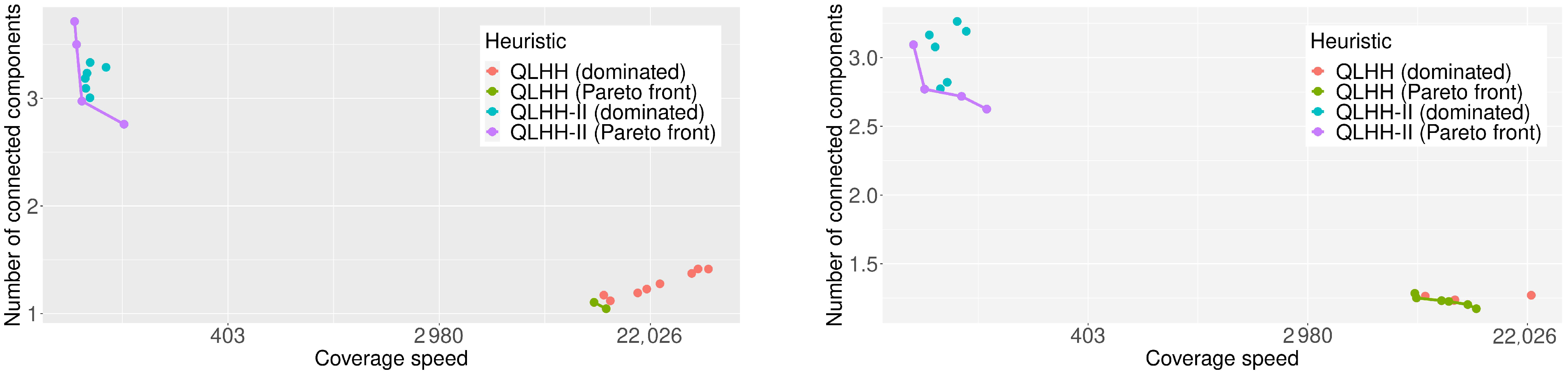
This section aims at comparing the current hyper-heuristic QLHH-II to the one it extends, i.e., QLHH. To compare both models, QLHH and QLHH-II have been trained on instances from class (15 × 15/10). QLHH uses the parameterisation provided used by Duflo et al. [31] while QLHH-II uses the parameterisation obtained after the factorial experiment described above. The generated heuristic has then been executed on several instances, ten times, from the same class. The solutions are represented according to both swarm metrics for two instances in Figure 8.

The results shown in Figure 8 are representative of the behaviour in other instances. It shows the Pareto fronts obtained by executing both generated heuristics ten times on two instances from the class (15 × 15/10). QLHH generated a heuristic that provides solutions with a low number of connected components, around 1.5. This is due to the fact that the scalarisation weights enhance the connectivity objective without making UAVs cover new vertices until a point where the weight for the coverage rate becomes too large. This explains why the coverage speed is extremely high for solutions obtained by the heuristic generated by QLHH. The heuristic generated by QLHH-II provides a poorer connectivity since the number of connected components is around 3, but also a much better coverage speed. For any instance, UAVs need between 100 and 150 units of time to cover 95% of the environment graph, while they need between 10,000 and 30,000 with the heuristic generated by QLHH.

By looking at Figure 8, QLHH-II may seem to focus on the coverage objective only, but this is not the case. This idea is induced by the good connectivity obtained by the heuristic generated by QLHH in comparison, but the solutions produced by the latter heuristic are practically unusable. Consequently, the heuristics generated by QLHH will not be used as a comparison for the stability experiment detailed below.

6.3. Stability

QLHH-II has been trained on instances from the (20 × 20/10) instance class. This class has been chosen since the number of UAVs is high enough to have a wide range of values for the connectivity objective. Moreover, the ratio of the number of vertices over the number of UAVs is good, so that UAVs are not constrained to fly together by the lack of free room. The generated heuristic has then been executed on other instance classes, i.e., (15 × 15/10), (20 × 20/5), (20 × 20/10), (20 × 20/15) and (25 × 25/10). The objective is not only to demonstrate its good performance on other instance classes with different numbers of UAVs and environment grid sizes but also to validate its good stability against heuristics from the state-of-the-art.

6.3.1. Training

This section presents the training process along with the evolution of the Pareto front, which depicts the convergence of the model and, therefore, justifies the training time. QLHH-II has been trained on 50 instances over 10 epochs, resulting in 500 episodes. The evolution of the three MO metrics during training is illustrated in Figure 9. In terms of IGD, the algorithm features a very fast convergence in the first episodes and then continues to improve at a slower pace. When considering HV, it appears that QLHH-II improves solutions steadily with a major increase around the 300th episode. With regard to the third metric, Δ, it converges until the 50th episode and then worsens. This might be explained by the fact that adding any new non-dominated to the front may completely disrupt the diversity.

6.3.2. Testing

For both WO and the generated heuristics, each UAV has a deterministic behaviour so they are not stochastic as are heuristics Φ and Φ-K. However, since UAVs move asynchronously, two executions on the same instance may provide two different solutions, which makes these two heuristics non-deterministic. Thus, all heuristics have been executed 30 times per instance, resulting in 30 solutions per instance. These distributions are compared according to their Pareto front using the three MO metrics defined in Section 5.1. A Wilcoxon signed-rank test is then used to assess the statistical significance of the results. The results of the latter test are displayed in three tables, one per MO metric (HV in

Table 3. Comparison between heuristics according to HV.

Instance Class		Heuristic
Grid	#UAVs	QLHH-II	WO	$\mathit{p}$-Value	Φ	$\mathit{p}$-Value	Φ-K0.05	$\mathbf{p}$-Value	Φ-K0.10	$\mathit{p}$-Value	Φ-K0.20	$\mathit{p}$-Value
15 × 15	10	$2.03\times {10}^1$ ±$3.97$	$1.92\times {10}^1$ ±$3.54$	$4.37\times {10}^{-4}$	$5.42$ ±$1.27$	$7.11\times {10}^{-15}$	$7.94$ ±$1.81$	$7.11\times {10}^{-15}$	$1.01\times {10}^1$ ±$2.03$	$7.11\times {10}^{-15}$	$1.40\times {10}^1$ ±$2.93$	$7.11\times {10}^{-15}$
20 × 20	05	$1.35\times {10}^1$ ±$3.01$	$1.48\times {10}^1$ ±$2.92$	$1.20\times {10}^{-2}$	$2.52$ ±$6.82\times {10}^{-1}$	$7.63\times {10}^{-6}$	$3.56$ ±$8.02\times {10}^{-1}$	$7.63\times {10}^{-6}$	$4.53$ ±$1.03$	$7.63\times {10}^{-6}$	$6.83$ ±$1.59$	$7.63\times {10}^{-6}$
20 × 20	10	$1.60\times {10}^1$ ±$4.61$	$1.75\times {10}^1$ ±$4.21$	$4.57\times {10}^{-2}$	$3.27$ ±$9.60\times {10}^{-1}$	$1.19\times {10}^{-7}$	$4.81$ ±$1.27$	$1.19\times {10}^{-7}$	$6.39$ ±$1.78$	$1.19\times {10}^{-7}$	$9.40$ ±$2.52$	$1.19\times {10}^{-7}$
20 × 20	15	$1.67\times {10}^1$ ±$3.69$	$1.63\times {10}^1$ ±$3.59$	$1.40\times {10}^{-1}$	$3.24$ ±$8.12\times {10}^{-1}$	$1.86\times {10}^{-9}$	$5.22$ ±$1.01$	$1.86\times {10}^{-9}$	$7.14$ ±$1.50$	$1.86\times {10}^{-9}$	$1.13\times {10}^1$ ±$2.50$	$1.86\times {10}^{-9}$
25 × 25	10	$9.88$ ±$2.62$	$1.40\times {10}^1$ ±$2.14$	$1.53\times {10}^{-5}$	$1.62$ ±$4.86\times {10}^{-1}$	$7.63\times {10}^{-6}$	$2.72$ ±$5.71\times {10}^{-1}$	$7.63\times {10}^{-6}$	$3.74$ ±$7.10\times {10}^{-1}$	$7.63\times {10}^{-6}$	$5.65$ ±$1.22$	$7.63\times {10}^{-6}$

, IGD in

Table 4. Comparison between heuristics according to IGD.

Instance Class		Heuristic
Grid	#UAVs	QLHH-II	WO	$\mathit{p}$-Value	Φ	$\mathit{p}$-Value	Φ-K0.05	$\mathit{p}$-Value	Φ-K0.10	$\mathit{p}$-Value	Φ-K0.20	$\mathit{p}$-Value
15 × 15	10	$3.74\times {10}^{-1}$ ±$1.46\times {10}^{-1}$	$8.99\times {10}^{-1}$ ±$2.92\times {10}^{-1}$	$3.54\times {10}^{-11}$	$2.40$ ±$1.62\times {10}^{-1}$	$7.11\times {10}^{-15}$	$1.99$ ±$1.98\times {10}^{-1}$	$7.11\times {10}^{-15}$	$1.64$ ±$1.70\times {10}^{-1}$	$7.11\times {10}^{-15}$	$1.11$ ±$1.50\times {10}^{-1}$	$7.11\times {10}^{-15}$
20 × 20	05	$6.08\times {10}^{-1}$ ±$3.23\times {10}^{-1}$	$1.25$ ±$4.08\times {10}^{-1}$	$1.58\times {10}^{-3}$	$2.57$ ±$2.21\times {10}^{-1}$	$7.63\times {10}^{-6}$	$2.35$ ±$2.09\times {10}^{-1}$	$7.63\times {10}^{-6}$	$2.16$ ±$1.85\times {10}^{-1}$	$7.63\times {10}^{-6}$	$1.69$ ±$1.72\times {10}^{-1}$	$7.63\times {10}^{-6}$
20 × 20	10	$6.68\times {10}^{-1}$ ±$3.27\times {10}^{-1}$	$1.15$ ±$5.13\times {10}^{-1}$	$1.26\times {10}^{-2}$	$2.58$ ±$2.55\times {10}^{-1}$	$1.19\times {10}^{-7}$	$2.26$ ±$2.51\times {10}^{-1}$	$1.19\times {10}^{-7}$	$1.97$ ±$2.49\times {10}^{-1}$	$1.19\times {10}^{-7}$	$1.50$ ±$2.52\times {10}^{-1}$	$1.19\times {10}^{-7}$
20 × 20	15	$5.09\times {10}^{-1}$ ±$2.00\times {10}^{-1}$	$1.32$ ±$3.25\times {10}^{-1}$	$9.31\times {10}^{-9}$	$2.51$ ±$2.12\times {10}^{-1}$	$1.86\times {10}^{-9}$	$2.14$ ±$1.58\times {10}^{-1}$	$1.86\times {10}^{-9}$	$1.78$ ±$1.55\times {10}^{-1}$	$1.86\times {10}^{-9}$	$1.14$ ±$1.57\times {10}^{-1}$	$1.86\times {10}^{-9}$
25 × 25	10	$8.60\times {10}^{-1}$ ±$3.73\times {10}^{-1}$	$1.52$ ±$5.57\times {10}^{-1}$	$6.58\times {10}^{-3}$	$2.72$ ±$1.95\times {10}^{-1}$	$7.63\times {10}^{-6}$	$2.47$ ±$1.85\times {10}^{-1}$	$7.63\times {10}^{-6}$	$2.20$ ±$2.18\times {10}^{-1}$	$7.63\times {10}^{-6}$	$1.74$ ±$2.40\times {10}^{-1}$	$7.63\times {10}^{-6}$

and Δ in

Table 5. Comparison between heuristics according to Δ.

Instance Class		Heuristic
Grid	#UAVs	QLHH-II	WO	$\mathit{p}$-Value	Φ	$\mathit{p}$-Value	Φ-K0.05	$\mathit{p}$-Value	Φ-K0.10	$\mathit{p}$-Value	Φ-K0.20	$\mathit{p}$-Value
15 × 15	10	$8.26\times {10}^{-1}$ ±$6.43\times {10}^{-2}$	$8.68\times {10}^{-1}$ ±$8.06\times {10}^{-2}$	$6.31\times {10}^{-3}$	$9.15\times {10}^{-1}$ ±$4.05\times {10}^{-2}$	$6.46\times {10}^{-10}$	$8.74\times {10}^{-1}$ ±$6.32\times {10}^{-2}$	$1.15\times {10}^{-4}$	$8.67\times {10}^{-1}$ ±$7.12\times {10}^{-2}$	$9.31\times {10}^{-3}$	$8.53\times {10}^{-1}$ ±$8.43\times {10}^{-2}$	$6.68\times {10}^{-2}$
20 × 20	05	$8.95\times {10}^{-1}$ ±$8.04\times {10}^{-2}$	$9.00\times {10}^{-1}$ ±$5.45\times {10}^{-2}$	$8.99\times {10}^{-1}$	$9.18\times {10}^{-1}$ ±$3.54\times {10}^{-2}$	$3.69\times {10}^{-1}$	$8.88\times {10}^{-1}$ ±$5.11\times {10}^{-2}$	$5.51\times {10}^{-1}$	$9.29\times {10}^{-1}$ ±$4.40\times {10}^{-2}$	$1.54\times {10}^{-1}$	$8.47\times {10}^{-1}$ ±$4.78\times {10}^{-2}$	$4.32\times {10}^{-2}$
20 × 20	10	$8.34\times {10}^{-1}$ ±$4.33\times {10}^{-2}$	$8.56\times {10}^{-1}$ ±$1.94\times {10}^{-1}$	$1.15\times {10}^{-2}$	$9.18\times {10}^{-1}$ ±$3.16\times {10}^{-2}$	$3.58\times {10}^{-7}$	$9.16\times {10}^{-1}$ ±$4.22\times {10}^{-2}$	$3.58\times {10}^{-7}$	$9.01\times {10}^{-1}$ ±$6.23\times {10}^{-2}$	$2.05\times {10}^{-4}$	$8.79\times {10}^{-1}$ ±$7.06\times {10}^{-2}$	$1.38\times {10}^{-2}$
20 × 20	15	$8.64\times {10}^{-1}$ ±$5.73\times {10}^{-2}$	$8.91\times {10}^{-1}$ ±$6.26\times {10}^{-2}$	$1.58\times {10}^{-1}$	$9.27\times {10}^{-1}$ ±$3.61\times {10}^{-2}$	$7.99\times {10}^{-6}$	$9.13\times {10}^{-1}$ ±$3.26\times {10}^{-2}$	$7.98\times {10}^{-4}$	$8.88\times {10}^{-1}$ ±$5.89\times {10}^{-2}$	$1.64\times {10}^{-2}$	$8.48\times {10}^{-1}$ ±$6.70\times {10}^{-2}$	$5.70\times {10}^{-1}$
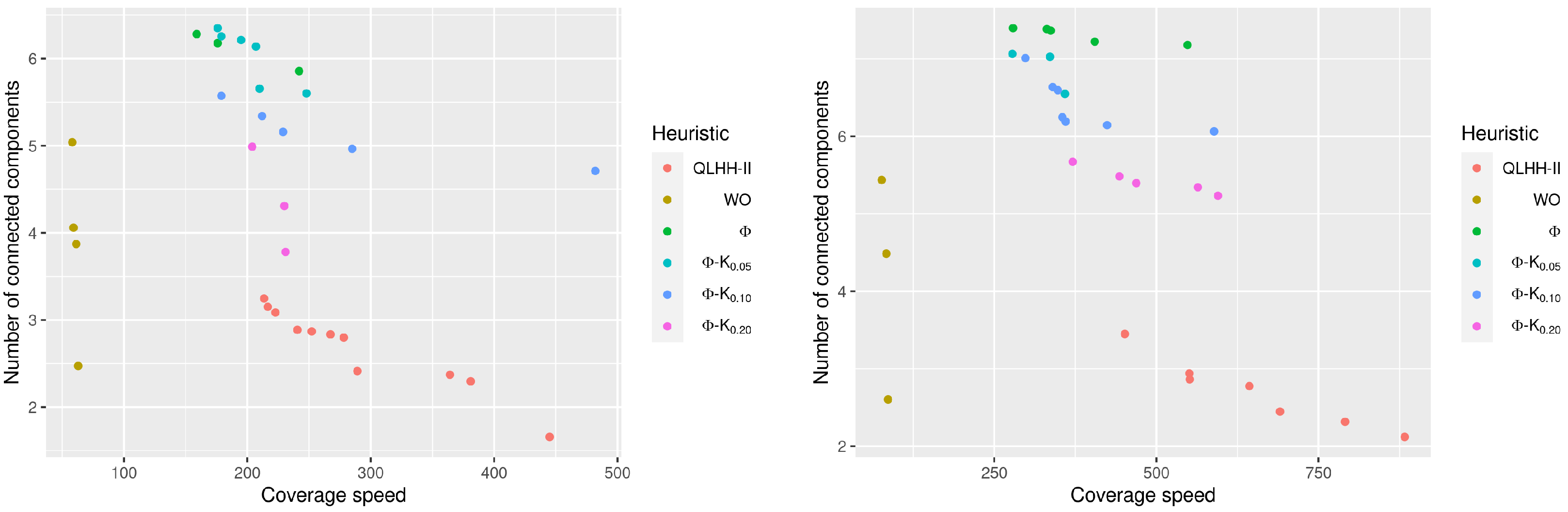
25 × 25	10	$8.42\times {10}^{-1}$ ±$2.84\times {10}^{-2}$	$8.64\times {10}^{-1}$ ±$8.88\times {10}^{-2}$	$2.46\times {10}^{-1}$	$9.46\times {10}^{-1}$ ±$2.84\times {10}^{-2}$	$7.63\times {10}^{-6}$	$9.40\times {10}^{-1}$ ±$3.88\times {10}^{-2}$	$7.63\times {10}^{-6}$	$9.24\times {10}^{-1}$ ±$4.21\times {10}^{-2}$	$7.63\times {10}^{-6}$	$9.26\times {10}^{-1}$ ±$3.80\times {10}^{-2}$	$7.63\times {10}^{-6}$

). For each table, a cell in dark blue means that the heuristic generated by QLHH-II outperforms the specific heuristic (column name) for the specific instance class (row name) with a 95% confidence. A light-blue cell means that the heuristic generated by QLHH-II provides better results on average but without statistical confidence.

According to the HV metric, the heuristic generated by QLHH-II outperforms all pheromone-based heuristics. However, for most of the instance classes, the WO heuristic provides better results with 95% confidence. This is an unexpected result when looking at its results in terms of IGD and Δ metrics. It indeed clearly appears that the generated heuristic outperforms WO for every instance class according to IGD and Δ. While these metrics, respectively, measure the convergence and the diversity of the front, the results in terms of HV values are not similarly competitive with respect to WO. This behaviour can be visualised in Figure 10, which displays the non-dominated solutions for two different instances. It can be observed that, despite a clear lack of diversity in the front of WO, its lowermost point is very distant from the other solutions (including the dominated ones), which in turn drastically increases the value of HV.

In terms of IGD, the heuristic generated by QLHH-II outperforms all other heuristics as presented in Table 4. It means that the non-dominated solutions provided by the generated heuristic are closer to the optimal front than other heuristics. This result is particularly good since the front provided by the generated heuristic has more points than other ones for most instances (see Figure 10).

This diversity in the Pareto fronts obtained with the QLHH-II generated heuristic is confirmed by the results according to the Spread metric (Δ) presented in Table 5. QLHH-II obtained fronts are, in the majority of cases, more diverse than the state-of-the-art heuristics. For some class, heuristic Φ-K, however, provides more diverse fronts, but with a 95% confidence only for the class (20 × 20/5).

Overall, except for some specific cases, the heuristic generated by QLHH-II outperforms the state-of-the-art heuristics according to the three MO metrics. By observing the fronts obtained with different heuristics (see Figure 10, for example), several aspects can be pointed out. First, in terms of convergence of the Pareto front, all of the pheromone-based heuristics are completely outperformed by the generated heuristic. Most of the solutions provided by heuristics Φ and Φ-K are dominated by solutions from the front of the generated heuristic. Another point is that the WO heuristic provides the best coverage results for every instance. However, it does not seem to consider the connectivity aspect of the swarm while that heuristic has been designed to balance the CCUS3O objectives. It shows that the limitation of the manual design is even more apparent when trying to deal with multi-objective optimisation problems. The last aspect is that the front obtained with the QLHH-II generated heuristic is generally the one containing the most solutions. This is an important feature since it shows that it is able to provide a larger set of well-performing solutions.

The main purpose of this experiment was to demonstrate the stability of the model. After training QLHH-II on instances from (20 × 20/10), the generated heuristic has shown very similar results after being executed on other instance classes. The class where the generated heuristic seems to be the least efficient is (20 × 20/5) in terms of diversity of the front. This is, however, not due to the density of the swarm compared to the swarm of the grid (fewer UAVs than during training) since the generated heuristic provides good results on instances from (25 × 25/10) where the grid is bigger than during training. The model is, thus, able to generate a heuristic without being overfitted by the dimension of the instance. The stability of the model is a very promising aspect, since it shows that the generated heuristic can perform well not only on unknown instances, but also in unknown situations and, therefore, dynamic environments.

7. Conclusions

This article introduced a novel approach for learning to optimise the coverage of an area by a swarm of UAVs, i.e., automating the design of swarming behaviours in the context of area coverage missions. As a first step, a multi-objective optimisation problem has been defined to formally describe the objectives of the task to cover an area with a swarm of UAVs. This problem, called the Coverage of a Connected-UAV Swarm with 3 Objectives (CCUS3O), considers the coverage rate, the coverage time and the swarm connectivity. A CCUS3O instance represents a scenario for an area coverage mission. To automatically obtain the distributed heuristics necessary to tackle CCUS3O, a novel hyper-heuristic has been developed. Based on multi-objective Q-learning, also referred to as QLHH-II, it has been experimented on a set of CCUS30 instances. 50 instances from the class (20 × 20/10) (10 UAVs on a 20 × 20 grid) have been used for the training. The generated heuristic has then been executed on 50 new instances of five different classes. The proposed hyper-heuristic has revealed a better convergence than existing techniques by generating a heuristic not only with better performance but also with more consideration of the multi-objective aspect. After processing a factorial experiment to determine an efficient parameterisation, experimental results demonstrate that while trained on a single instance class, the generated heuristic has shown to outperform on other classes a manually designed problem-specific heuristic along with state-of-the-art techniques designed for the coverage by a swarm of UAVs. In addition, empirical evidence of the good stability of the model and the better balance obtained on both objectives, coverage speed and swarm connectivity, has been provided.

Future works will first consist of analysing other types of scalarisation techniques, such as Chebyshev. In the next step, following the empirically assessed good stability of the model, i.e., ability to generate a heuristic that performs well in unknown instances, the final objective of this work will be to study QLHH-II in dynamic environments. In a later stage, QLHH-II will be extended to tackle more diverse classes of problems.

References

- Birattari, M.; Ligot, A.; Bozhinoski, D.; Brambilla, M.; Francesca, G.; Garattoni, L.; Garzón Ramos, D.; Hasselmann, K.; Kegeleirs, M.; Kuckling, J.; et al. Automatic Off-Line Design of Robot Swarms: A Manifesto. Front. Robot. AI 2019, 6, 59. [Google Scholar] [CrossRef] [PubMed]
- Silva, F.; Duarte, M.; Correia, L.; Oliveira, S.M.; Christensen, A.L. Open Issues in Evolutionary Robotics. Evol. Comput. 2016, 24, 205–236. [Google Scholar] [CrossRef] [PubMed]
- Francesca, G.; Birattari, M. Automatic Design of Robot Swarms: Achievements and Challenges. Front. Robot. AI 2019, 3, 29. [Google Scholar] [CrossRef]
- Arnold, R.; Carey, K.; Abruzzo, B.; Korpela, C. What is A Robot Swarm: A Definition for Swarming Robotics. In Proceedings of the 2019 IEEE 10th Annual Ubiquitous Computing, Electronics & Mobile Communication Conference, New York, NY, USA, 10–12 October 2019; pp. 0074–0081. [Google Scholar]
- Brambilla, M.; Ferrante, E.; Birattari, M.; Dorigo, M. Swarm robotics: A review from the swarm engineering perspective. Swarm Intell. 2013, 7, 1–41. [Google Scholar] [CrossRef]
- Schranz, M.; Umlauft, M.; Sende, M.; Elmenreich, W. Swarm Robotic Behaviors and Current Applications. Front. Robot. AI 2020, 7, 36. [Google Scholar] [CrossRef] [PubMed]
- Cabreira, T.M.; Brisolara, L.B.; Ferreira, P.R., Jr. Survey on Coverage Path Planning with Unmanned Aerial Vehicles. Drones 2019, 3, 4. [Google Scholar] [CrossRef]
- Siemiatkowska, B.; Stecz, W. A Framework for Planning and Execution of Drone Swarm Missions in a Hostile Environment. Sensors 2021, 21, 4150. [Google Scholar] [CrossRef] [PubMed]
- Semiz, F.; Polat, F. Solving the area coverage problem with UAVs: A vehicle routing with time windows variation. Robot. Auton. Syst. 2020, 126, 103435. [Google Scholar] [CrossRef]
- Nouyan, S.; Campo, A.; Dorigo, M. Path formation in a robot swarm: Self-organized strategies to find your way home. Swarm Intell. 2008, 2, 1–23. [Google Scholar] [CrossRef]
- Ducatelle, F.; Di Caro, G.A.; Pinciroli, C.; Mondada, F.; Gambardella, L.M. Communication assisted navigation in robotic swarms: Self-organization and cooperation. In Proceedings of the 2011 IEEE/RSJ International Conference on Intelligent Robots and Systems, San Francisco, CA, USA, 25–30 September 2011; pp. 4981–4988. [Google Scholar]
- Sun, X.; Liu, T.; Hu, C.; Fu, Q.; Yue, S. ColCOS Φ: A Multiple Pheromone Communication System for Swarm Robotics and Social Insects Research. In Proceedings of the 2019 IEEE 4th International Conference on Advanced Robotics and Mechatronics (ICARM), Toyonaka, Japan, 3–5 July 2019; pp. 59–66. [Google Scholar]
- Na, S.; Qiu, Y.; Turgut, A.E.; Ulrich, J.; Krajník, T.; Yue, S.; Lennox, B.; Arvin, F. Bio-inspired artificial pheromone system for swarm robotics applications. Adapt. Behav. 2021, 29, 395–415. [Google Scholar] [CrossRef]
- Liu, T.; Sun, X.; Hu, C.; Fu, Q.; Isakhani, H.; Yue, S. Investigating Multiple Pheromones in Swarm Robots—A Case Study of Multi-Robot Deployment. In Proceedings of the 2020 5th International Conference on Advanced Robotics and Mechatronics (ICARM), Shenzhen, China, 18–21 December 2020; pp. 595–601. [Google Scholar]
- Liu, T.; Sun, X.; Hu, C.; Fu, Q.; Yue, S. A Multiple Pheromone Communication System for Swarm Intelligence. IEEE Access 2021, 9, 148721–148737. [Google Scholar] [CrossRef]
- Kuiper, E.; Nadjm-Tehrani, S. Mobility Models for UAV Group Reconnaissance Applications. In Proceedings of the 2006 International Conference on Wireless and Mobile Communications (ICWMC’06), Bucharest, Romania, 29–31 July 2006; IEEE: Bucharest, Romania, 2006; p. 33. [Google Scholar]
- Rosalie, M.; Danoy, G.; Chaumette, S.; Bouvry, P. Chaos-enhanced mobility models for multilevel swarms of UAVs. Swarm Evol. Comput. 2018, 41, 36–48. [Google Scholar] [CrossRef]
- Danoy, G.; Brust, M.R.; Bouvry, P. Connectivity Stability in Autonomous Multi-level UAV Swarms for Wide Area Monitoring. In Proceedings of the 5th ACM Symposium on Development and Analysis of Intelligent Vehicular Networks and Applications—DIVANet ’15, Cancun, Mexico, 2–6 November 2015; ACM Press: Cancun, Mexico, 2015; pp. 1–8. [Google Scholar] [CrossRef]
- Brust, M.R.; Zurad, M.; Hentges, L.; Gomes, L.; Danoy, G.; Bouvry, P. Target Tracking Optimization of UAV Swarms Based on Dual-Pheromone Clustering. In Proceedings of the 3rd IEEE International Conference on Cybernetics, Exeter, UK, 21–23 June 2017; pp. 1–8. [Google Scholar]
- Hunt, E.R.; Jones, S.; Hauert, S. Testing the limits of pheromone stigmergy in high-density robot swarms. R. Soc. Open Sci. 2019, 6, 190225. [Google Scholar] [CrossRef] [PubMed]
- Burke, E.K.; Gendreau, M.; Hyde, M.; Kendall, G.; Ochoa, G.; Özcan, E.; Qu, R. Hyper-heuristics: A survey of the state of the art. J. Oper. Res. Soc. 2013, 64, 1695–1724. [Google Scholar] [CrossRef]
- Epitropakis, M.G.; Burke, E.K. Hyper-heuristics. In Handbook of Heuristics; Martí, R., Pardalos, P.M., Resende, M.G.C., Eds.; Springer International Publishing: Cham, Switzerland, 2018; pp. 489–545. [Google Scholar]
- Burke, E.K.; Hyde, M.R.; Kendall, G.; Ochoa, G.; Özcan, E.; Woodward, J.R. A Classification of Hyper-Heuristic Approaches: Revisited. In Handbook of Metaheuristics; Gendreau, M., Potvin, J.Y., Eds.; Springer International Publishing: Cham, Switzerland, 2019; Volume 272, pp. 453–477. [Google Scholar]
- Li, K.; Malik, J. Learning to Optimize. In Proceedings of the 5th International Conference on Learning Representations, ICLR 2017, Toulon, France, 24–26 April 2017. [Google Scholar]
- Cowling, P.; Kendall, G.; Soubeiga, E. A Hyperheuristic Approach to Scheduling a Sales Summit. In Practice and Theory of Automated Timetabling III; Goos, G., Hartmanis, J., van Leeuwen, J., Burke, E., Erben, W., Eds.; Springer: Berlin/Heidelberg, Germany, 2001; Volume 2079, pp. 176–190. [Google Scholar]
- Birattari, M.; Ligot, A.; Francesca, G. AutoMoDe: A Modular Approach to the Automatic Off-Line Design and Fine-Tuning of Control Software for Robot Swarms. In Automated Design of Machine Learning and Search Algorithms; Pillay, N., Qu, R., Eds.; Natural Computing Series; Springer International Publishing: Cham, Switzerland, 2021; pp. 73–90. [Google Scholar]
- Ligot, A.; Cotorruelo, A.; Garone, E.; Birattari, M. Towards an Empirical Practice in Off-line Fully-automatic Design of Robot Swarms. IEEE Trans. Evol. Comput. 2022, 1. [Google Scholar] [CrossRef]
- Yu, S.; Aleti, A.; Barca, J.C.; Song, A. Hyper-heuristic Online Learning for Self-assembling Swarm Robots. In Computational Science—ICCS 2018; Shi, Y., Fu, H., Tian, Y., Krzhizhanovskaya, V.V., Lees, M.H., Dongarra, J., Sloot, P.M.A., Eds.; Springer International Publishing: Berlin/Heidelberg, Germany, 2018; Volume 10860, pp. 167–180. [Google Scholar]
- Yu, S.; Song, A.; Aleti, A. A Study on Online Hyper-heuristic Learning for Swarm Robots. In Proceedings of the IEEE Congress on Evolutionary Computation, Wellington, New Zealand, 10–13 June 2019; pp. 2721–2728. [Google Scholar]
- Nagavalli, S.; Chakraborty, N.; Sycara, K. Automated sequencing of swarm behaviors for supervisory control of robotic swarms. In Proceedings of the 2017 IEEE International Conference on Robotics and Automation (ICRA), Singapore, 29 May–3 June 2017; pp. 2674–2681. [Google Scholar]
- Duflo, G.; Danoy, G.; Talbi, E.G.; Bouvry, P. A Q-Learning Based Hyper-Heuristic for Generating Efficient UAV Swarming Behaviours. In Proceedings of the Intelligent Information and Database Systems; Nguyen, N.T., Chittayasothorn, S., Niyato, D., Trawiński, B., Eds.; Springer International Publishing: Cham, Switzerland, 2021; pp. 768–781. [Google Scholar] [CrossRef]
- Duflo, G.; Danoy, G.; Talbi, E.G.; Bouvry, P. Automating the Design of Efficient Distributed Behaviours for a Swarm of UAVs. In Proceedings of the 2020 IEEE Symposium Series on Computational Intelligence (SSCI), Canberra, Australia, 1–4 December 2020; pp. 489–496. [Google Scholar]
- Van Moffaert, K.; Drugan, M.M.; Nowe, A. Scalarized multi-objective reinforcement learning: Novel design techniques. In Proceedings of the 2013 IEEE Symposium on Adaptive Dynamic Programming and Reinforcement Learning (ADPRL), Singapore, 16–19 April 2013; pp. 191–199. [Google Scholar]
- Brust, M.R.; Frey, H.; Rothkugel, S. Dynamic Multi-Hop Clustering for Mobile Hybrid Wireless Networks. In Proceedings of the 2nd International Conference on Ubiquitous Information Management and Communication, ICUIMC ’08, Suwon, Korea, 31 January–1 February 2008; Association for Computing Machinery: New York, NY, USA, 2008; pp. 130–135. [Google Scholar] [CrossRef]
- Varrette, S.; Bouvry, P.; Cartiaux, H.; Georgatos, F. Management of an Academic HPC Cluster: The UL Experience. In Proceedings of the 2014 International Conference on High Performance Computing & Simulation (HPCS 2014), Bologna, Italy, 21–25 July 2014; pp. 959–967. [Google Scholar]