Machine Learning and Sustainable Mobility: The Case of the University of Foggia (Italy)

Abstract

Thanks to the development of increasingly sophisticated machine-learning techniques, it is possible to improve predictions of a particular phenomenon. In this paper, after analyzing data relating to the mobility habits of University of Foggia (UniFG) community members, we apply logistic regression and cross validation to determine the information that is missing in the dataset (so-called imputation process). Our goal is to make it possible to obtain the missing information that can be useful for calculating sustainability indicators and that allow the UniFG Rectorate to improve its sustainable mobility policies by encouraging methods that are as appropriate as possible to the users’ needs.

1. Introduction

The problem of sustainable mobility choices involves more and more public and private organizations. As defined by Banister [1], implementing the sustainable-mobility paradigm requires intervention by a series of people who can develop policies capable of reducing car dependence. Sustainable mobility plays a fundamental role [2] in community development from the economic, environmental, and social points of view. In particular, a sustainable transport system should guarantee efficient travel to all users and an ecological means of transport while maintaining certain levels of economy and public health [3,4,5].

Decision makers’ choices recently have been oriented toward reducing pollutant emissions in the most congested urban areas by introducing green vehicles, such as bicycles or scooters. However, these means of transport represent only a part of cities’ environmental development [6]. The decisions taken include introducing car-sharing systems, integrated transport systems, bike-sharing systems, bus prioritization, and free public transport [7,8,9,10]. The goal of the top organizational officers of the university is to develop a system for evaluating the mobility choices of community members (in this specific case, the members of the University of Foggia) based on the distance covered and the types of vehicle used. Such a system would allow each member to know whether or not he/she is respecting the objectives set by the community policymaker and consequently to try to improve himself/herself to meet the established parameters. With this paper, we propose a system based on logistic regression and a k-fold cross validation (trained on the dataset obtained in [11]) that allow, in an automatic way, to obtain the missing information of a variable (so-called feature). This is because the necessary data, such as means of transport, travel duration, and travel days, are obtained through a questionnaire. The presence of missing data or errors in the compilation can quickly occur. Our goal is to use a so-called imputation method to ensure that missing data are replaced by new predicted values. This imputation process can allow the creation of an automated system that, based on only a few answers, allows to impute values relative to other variables not requested directly based on its training.

The present paper is structured as follows. The following section describes the variables present in the data set collected from the academic community, and the most critical features are analyzed through factor analysis and machine learning. Section 3 presents a possible application of these features to determine the emission levels of each UniFG member. Finally, in Section 4, some conclusions are drawn.

Literature Review

Researchers recently have used ML algorithms to solve many problems, ranging from the industrial to the economic spheres. Within sustainable mobility, several authors have proposed models whose objectives range from determining the shortest route with a means of transport to determining which means to choose based on certain features. For example, using a random forest, Zhou et al. [12] determined the seasonality in the choice of bike sharing, as compared to taxis, in Chicago. Basu and Ferreira [13] used neural networks to identify the factors influencing the choice of a type of means of transport. Yang et al. [14] proposed a deep learning system to improve the forecast of the demand for bikes in bike-sharing systems. Using machine learning algorithms, Tang et al. [15] could predict passengers’ bus stops. Migliore et al. [16] proposed a system based on ML to optimize parking prices in Palermo. In a support vector machine (SVM) study, Liang et al. [17] predicted household travel modes based on various factors. Asensio et al. [18] solved several issues using text-mining algorithms on electric car charging stations reviews. Nandal et al. [19] highlighted the role of neural networks in improving infrastructure deterioration. Finally, Hasan et al. [20] developed a system capable of reducing pollutant emissions from self-driving vehicles by 80%. Alternatively, given the very high applicability of machine/deep learning techniques to any sector, Kaplan et al. [21] used a neural network with long short-term memory (LSTM) cell to perform the detection of faults in electric vehicles (EVs), demonstrating how this approach is superior in terms of accuracy compared to the techniques used previously and highlighting the contribution of Deep Learning in the fault diagnosis of EVs. Ghamisi et al. [22] proposed a multisensor feature fusion approach for sustainable mining, using convolutional neural networks (CNNs) to extract information from sensors and use them in the classification phase, demonstrating how this approach produces results with high classification accuracy. Delnevo et al. [23] proposed a combined approach between the Internet of Things (IoT) and deep learning techniques to monitor and count the presence of people on beaches and coasts, highlighting the approach’s usefulness and the accuracy levels achieved. Adeodato et al. [24] proposed a time series methodology based on MLP networks to obtain more robust results. Xiao et al. [25] combined the autoregressive moving average with the least squares support vector machine (ARI-MA-LS-SVM) model to improve prediction in financial markets. Zaccagnino et al. [26,27] studied human online activities and proposed automatic ML-based methods to provide privacy awareness to users and total control over their data. Liu et al. [28] proposed combinations of CNN architectures for high-resolution segmentation to improve the calculation of the distance between vehicles via graphical analysis. Finally, Jin et al. [29] used the attention mechanism to improve prediction in financial markets, combining it with empirical model decomposition (EDM) and LSTM-type cells.

In this paper, we will use ML algorithms to prepare an automatic imputation helpful system, for example, for estimating the emissions of UniFG members. In particular, this method will allow us to exploit readily available data through a brief questionnaire to estimate other missing data, which would be more challenging to obtain for each community member in practice. The birth of statistical techniques in the presence of missing data can be traced back to some authors, such as Madow et al. [30], in which the authors introduced the problem of missing data substitution. Rubin [31] proposed a framework based on the Bayesian approach for missing values. However, Little and Rubin [32] proposed using different statistical techniques in the presence of missing values. Laird [33] considered the use of likelihood-based analyses for longitudinal data with missing responses, both from the ease of implementation and appropriateness gave the non-response mechanism. Ibrahim [34] considered the presence of missing values (assumed as random) in the class of generalized linear models (GLMs); Horton and Laird [35], again with a view to GLMs, proposed a method that considers incomplete covariates. More recently, Raghunathan et al. [36] evaluated and described a series of procedures for imputation of missing values obtained from a sequence of regressions of different types (linear, logistic, and Poisson), motivated by multiple imputation analyses. Based on the tasks introduced by Rubin [37], van Buuren [38] defined a model for multivariate imputation in a convenient variable-by-variable manner, specifying a conditional model. Horton and Lipsitz [39] considered multiple imputations and, considering regression as a method, evaluate a series of statistical packages to implement the procedure. Jerez et al. [40] compared techniques of statistical imputation (e.g., multiple imputation) with imputation based on machine learning (multi-layer perceptron (MLP), self-organization maps (SOM) and k-nearest neighbor (k-NN)), demonstrating how the latter outperforms the classic methods. García-Laencina et al. [41] analyzed the problem of missing values in pattern classification tasks focusing on machine learning techniques for imputation. Silva-Ramírez et al. [42] proposed an automatic imputation system based on neural networks for missing values, combining MLP and k-NN, demonstrating how this system improves performance. Templeton et al. [43] presented an integrated imputation approach that mitigates the problems related to missing values, based on deriving an imputation model for each low-sample variable that leverages information available in large-sample sized inputs called RIOSSE (regression imputation optimizing sample size and emulation). Finally, Lin et al. [44] decided to enhance the techniques for imputation and used deep learning tools, such as deep neural networks (DNNs) and deep belief networks (DBNs) in the case of continuous missing values, demonstrating how deep networks obtain better results than classical models and of machine learning.

2. Materials and Methods

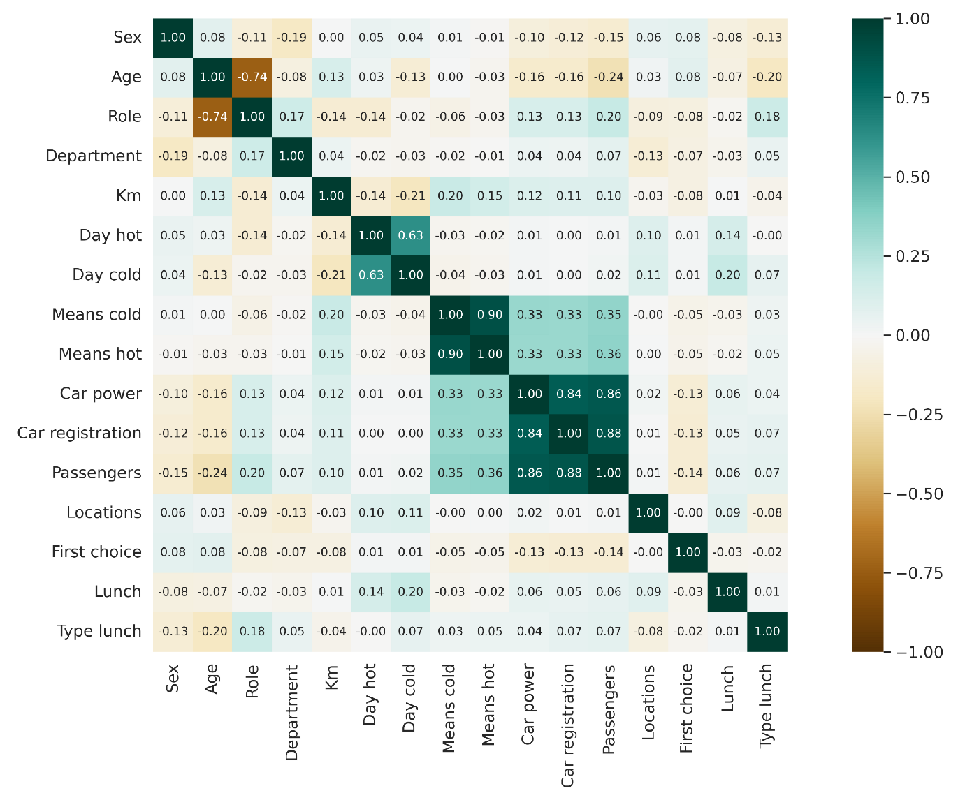
2.1. Dataset Description

The first step in understanding the habits among UniFG members is to consider the most significant possible number of variables detected during the survey [11]. This dataset contains information on the mobility habits of students, teachers, and technical-administrative staff belonging to the six departments of the University of Foggia. It was submitted to members via email and contains 2998 observations (after the cleanup process). In addition, it contains the following features shown in

Table 1. Description of the features in the dataset.

Feature	Description
Sex	Sex of respondents
Age	Age of respondents
Role	Role within the university
Department	Respondent department
Distance	Kilometers covered by respondents (round trip)
Min	Time taken to reach the department
Day hot	Number of days (hot season) that the respondent goes to university
Day cold	Number of days (cold season) that the respondent goes to university.
Means cold	Means of transport (cold season) used to get to the university
Means hot	Means of transport (hot season) used to get to the university
Car power	Power supply of the car (if it has been chosen as a means of transport)
Car registration	Year of registration of the car
Passengers	Number of passengers carried during the car journey
Locations	Moving to other university locations (other than your own department)
First choice rent	First choice alternative solutions for clean mobility
Second choice rent	Second choice alternative solutions for clean mobility
Third choice rent	Third choice alternative solutions for clean mobility
Fourth choice rent	Fourth choice alternative solutions for clean mobility
Lunch	Number of times the respondent has lunch at the university
Type lunch	Type of lunch eaten at the university (brought from home or purchased)

.

A priori, we can consider some information fundamental (especially for the calculation of emissions), such as the following:

• The distance in kilometers that the respondents claim to travel;
• The frequency at which the respondents go to their reference facility per weekly;
• Whether it is the hot or cold season, which affects both the number of weeks of activity and different modes of travel;
• The mode of transport used.

Notably, of these four parameters considered, the season is crucial when considering its implications on the other parameters. For this reason, we considered two partial datasets with only the data relating to each chosen season for calculating the seasonal kilometers. Furthermore, because these partial datasets were aimed at calculating emissions, the records of all the respondents who indicated that they used travel methods without significant emissions (walking, cycling, and riding an electric scooter) for each period considered were eliminated. The result of this operation was two datasets, “hot season km” and “cold season km”, which contain 2385 and 2517 records, respectively. Finally, for a calculation that considers the peculiarities of the different travel modes, it is necessary to obtain a single distinct kilometer value for each travel mode. The formula used to calculate the single kilometer values was as follows:

$$K{M}_{sm}=\sum _{i=1}^{n_{sm}}{D_{a/r}}_i·F{R}_i·SE{T}_i$$

(1)

where $K{M}_{sm}$ is the total kilometers traveled in season s by those who adopted travel method m; $n_{sm}$ is the total number of respondents who adopted travel method m in season s; $D_{a/r}$ is the round-trip distance traveled in kilometers to reach the university structure; $FR$ is the weekly travel frequency in season s; and $SET$ is the average number of weeks of lessons in season s. The kilometers traveled with the relative means of transport allow the calculation of the emissions in a closed formula [45,46,47]. Our goal is to allow this calculation to be possible even without some information (but extractable from similar data).

2.2. Data Preparation

First, we can make manipulations of the data. Many features in Table 1 are categorical, and the rest are numeric. Our goal was to understand which variables to use so that it is possible to reduce the number of features while maintaining a certain acceptable variance level. We can transform categorical variables into numerical ones via one-hot encoding for data that do not require a relationship between labels (e.g., sex, role, department, and type lunch) and via LabelEncoder for those in which there is a natural order (e.g., car power, car registration, and age), through sklearn (in Python). Furthermore, since it is advisable to standardize the data to carry out analyses, we use a StandardScaler (always in sklearn). We know that the variable that indicates the travel time (Min) cannot be considered since it includes times that do not fall within the calculation of emissions (linked to the structure of the questionnaire made to obtain the dataset). For this reason, trip duration from one’s home to the department was eliminated a priori, as were the second, third, and fourth choices of alternative sustainable mobility solutions (second-, third-, and fourth-choice rent) since we assumed that the first choice was the most representative. At this point, the dataset comprised 16 features describing transportation by the academic community.

To better understand the links between the different features, we can represent their Pearson’s correlations via a heat map, as shown in Figure 1.

Table 2. Significance values (p-values) of the correlation values (lower the better).

	Sex	Age	Role	Dept	Km	Day Hot	Day Cold	Means Cold	Means Hot	Car Power	Car reg.	Passengers	Locations	First Choice	Lunch	Type Lunch
Sex	0	0	0	0	0.875	0.0035	0.0162	0.5056	0.4761	0	0	0	0.0004	0	0	0
Age	0	0	0	0	0	0.0632	0	0.9905	0.0925	0	0	0	0.1571	0	0.0001	0
Role	0	0	0	0	0	0	0.1954	0.0014	0.1465	0	0	0	0	0	0.2641	0
Dept	0	0	0	0	0.0176	0.3117	0.0907	0.397	0.6989	0.0239	0.0543	0.0001	0	0	0.0631	0.005
Km	0.875	0	0	0.0176	0	0	0	0	0	0	0	0	0.096	0	0.6761	0.0168
Day hot	0.0035	0.0632	0	0.3117	0	0	0	0.1269	0.3498	0.4339	0.7868	0.6469	0	0.5534	0	0.9799
Day cold	0.0162	0	0.1954	0.0907	0	0	0	0.0195	0.1495	0.6361	0.8489	0.241	0	0.5256	0	0.0001
Means cold	0.5056	0.9905	0.0014	0.397	0	0.1269	0.0195	0	0	0	0	0	0.8642	0.0058	0.0589	0.0554
Means hot	0.4761	0.0925	0.1465	0.6989	0	0.3498	0.1495	0	0	0	0	0	0.874	0.0135	0.261	0.0121
Car power	0	0	0	0.0239	0	0.4339	0.6361	0	0	0	0	0	0.3192	0	0.0013	0.0288
Car registration	0	0	0	0.0543	0	0.7868	0.8489	0	0	0	0	0	0.6767	0	0.0049	0.0002
Passengers	0	0	0	0.0001	0	0.6469	0.241	0	0	0	0	0	0.4477	0	0.0005	0
Locations	0.0004	0.1571	0	0	0.096	0	0	0.8642	0.874	0.3192	0.6767	0.4477	0	0.7958	0	0
First choice	0	0	0	0	0	0.5534	0.5256	0.0058	0.0135	0	0	0	0.7958	0	0.0628	0.1915
Lunch	0	0.0001	0.2641	0.0631	0.6761	0	0	0.0589	0.261	0.0013	0.0049	0.0005	0	0.0628	0	0.5154
Type lunch	0	0	0	0.005	0.0168	0.9799	0.0001	0.0554	0.0121	0.0288	0.0002	0	0	0.1915	0.5154	0

shows the significance levels of the various correlations (p-value), from which it is possible to extract the most important relationships between the variables and how these are statistically significant (e.g., car registration, passengers, car power, age, and role). Of course, many of these correlations are conceivable a priori, such as the strong link between variables that explain the means of transport during the two seasons (as also highlighted by the significance levels).

2.3. Machine Learning Imputation

After making the dataset usable for different analyses, we can proceed to the imputation process through machine learning. In order to use this system to predict the emissions of pollutants, we need to consider what the missing features might be. For example, gender, age, role and department can be automatically extracted from the respondents since the questionnaire would be submitted directly through a management system that requires authentication. Instead, for some features that can be fundamental (such as those relating to the means of transport), it is necessary to prepare a system that determines them in case there are missing values.

The classification was the reference task for the analyses. Because these are multi-class classifications, we used logistic regression with the one-vs-rest (OvR) training algorithm in Python. In this way, logistic regression estimates the probability of an event occurring, limiting the variation of the dependent variable to the $(0,1)$ interval. The equation of the logistic function is of the type

$$y=\frac{1}{1+e^{-({\beta }_0+{\beta }_{1}x)}}$$

(2)

where ${\beta }_0$ and ${\beta }_1$ are the intercept and the rate parameter respectively, generally estimated via maximum likelihood estimation (MLE). In all cases, the training and test sets were divided into 70% and 30% portions, and a stratified 10-fold cross validation was performed to avoid over-fitting problems. To evaluate the goodness of the prediction, we report some indicators such as accuracy, precision, recall, $R^2$-score, Mean Absolute Percentage Error (MAPE), F1-score and F2-score. The predictive analyses were as follows:

• Prediction of the type of car fuel (the variable [car power]) used for moving (precisely the different types of petrol or diesel fuel) based on the variables [age, sex, department, role, distance, day cold, means cold, locations]. The accuracy, after cross validation, was 79.10% with a standard deviation of 1.5% ($R^2=69.7\%$, MAPE $=0.31$, precision $=0.1768$, recall $=0.2156$, F1 $=0.1922$, F2 $=0.7664$);
• Prediction of the car registration period (variable [car registration]) based on the variables [age, sex, role, department, distance, day cold, means cold, locations, car power (previously determined)]. The accuracy, after cross validation, was 75.70% with a standard deviation of 0.7% ($R^2=74.6\%$, MAPE $=0.41$, precision $=0.1685$, recall $=0.1965$, F1 $=0.1610$, F2 $=0.7313$);
• Prediction of the means of transport used in the hot season (variable [means hot]) based on the variables [age, sex, role, department, distance, day cold, means cold, car registration, car power (previously determined)]. The accuracy, after cross validation, was 91.30% with a standard deviation of 1.7% ($R^2=82.1\%$, MAPE $=0.34$, precision $=0.5047$, recall $=0.5180$, F1 $=0.5106$, F2 $=0.8697$);
• In the same way, prediction of the means of transport used in the cold season (variable [means cold]) based on the variables [age, sex, role, department, distance, day hot, means hot, car registration, car power (previously determined)]. The accuracy, after cross validation, was 90.70% with a standard deviation of 1.5% ($R^2=80.3\%$, MAPE $=35\%$, precision $=0.4574$, recall $=0.4386$, F1 $=0.4623$, F2 $=0.8335$).

The features considered in the various cases were chosen on the basis of the correlation levels and their statistical significance. It is evident that the above are the best predictions for imputation (with the highest accuracy) but that they require some features to be obtained, often high. If, for example, we wanted to determine the car fuel variable but were in the absence of the distance variable, the imputation could still be carried out but with lower accuracy.

2.4. Factor Analysis

Using the method to replace missing value may be interesting to reflect on a subsequent application of the data generated (which thus complete the necessary features) and those already present for the prediction of pollutants, for example. In particular, we can think of reducing the dimensionality of the dataset so that once the objective feature (the so-called y) is obtained, it is easier to use a lower number of factors. We tried to reduce the dimensionality of the dataset through factor analysis, considering the 12 features (except for those that have undergone one-hot encoding, and are therefore not optimal). This analysis also highlighted the links between the different features (described through the loadings), and was carried out also in Python through the FactorAnalyzer package (https://factor-analyzer.readthedocs.io/en/latest/, accessed on 1 May 2022). For this factor analysis, we opted for the 6-factor reduction with Varimax rotation, which explains 81.23% of the total variance.

As we can see in

Table 3. Factor loadings.

	Factor
Feature	1	2	3	4	5	6
Age	−0.015	0.006	−0.020	0.983	0.069	−0.005
Distance	0.066	0.109	−0.129	−0.094	0.599	−0.026
Day hot	0.004	−0.009	0.861	0.057	−0.044	0.149
Day cold	0.001	−0.007	0.674	−0.102	−0.168	0.293
Means cold	0.195	0.957	−0.009	0.014	0.122	−0.033
Means hot	0.207	0.892	−0.007	0.009	0.063	−0.009
Car power	0.890	0.156	0.011	−0.033	0.076	0.039
Car registration	0.912	0.149	0.004	−0.032	0.059	0.022
Passengers	0.928	0.175	0.010	−0.107	0.055	0.040
Locations	0.010	0.005	0.086	0.032	−0.030	0.177
First choice	−0.130	−0.011	0.010	0.069	−0.122	−0.036
Lunch	0.042	−0.032	0.085	−0.066	0.064	0.482

(which highlights the factor loadings), the variables with the highest loadings (>0.5) were related to the means of transport, the characteristics of these means, and the number of passengers, especially for the first factor loadings. For the second factor, the variables with the highest loadings were related to season of use. In this way, we replaced the features with a reduced number of factors that describe the entire dataset while accepting a certain level of information loss. Not only the reduction of dimensionality, but the factor analysis allows us to express an order relationship in the importance of the different features based on their link with the factors (expressed by the loadings). In this case, since the first factor highlights the highest loadings in the features on the characteristics of the means of transport, we can say that these are the most characteristic of the dataset, followed by the features on the season and those on the characteristics of the respondents. To this, we can add the analysis of communalities, always obtained from the factor analysis, which represents the sum of the squared loadings for each variable (where a value close to 1 indicates more significant variance and, therefore, importance). The communalities are represented in

Table 4. Communalities.

Feature	Age	Distance	Day Hot	Day Cold	Means c.	Means h.	Car Power	Car Regis.	Passengers	Locations	First c.	Lunch
Communality	0.99	0.40	0.77	0.58	0.97	0.84	0.82	0.86	0.90	0.04	0.03	0.25

. This supports the choice of variables made earlier in the logistic regression.

3. Results

The use of the imputation technique is, as mentioned, aimed at replacing those possible missing values that allow an automatic analysis to be carried out. For example, if data on emissions of CO₂ equivalent are available, the imputation would make it possible to predict some fundamental values necessary to classify a possible range of emissions for a new respondent not present in the dataset.

Information on age, gender, department, role, and residence for each subject can be acquired through the UniFG member management system (ESSE3 platform). However, the city of residence is not a functional variable since a person residing in a particular city could decide to move to Foggia. Therefore, one solution could be to periodically update the ESSE3 section relating to the domicile to track how the issue quantity can vary by subject over a certain period. In this way, because we are aware of the department to which each subject belongs and his or her domicile, the distance between these two points represents the distance in kilometers that the subject will travel with a certain vehicle.

To obtain information on means of transport (in particular car), it is possible to enter a brief questionnaire to ESSE3 with a single question, such as, “Do you use a car to go to the university? Yes/No.” This question may be mandatory for new subjects wishing to enroll at the university but voluntary for those already enrolled, thus minimizing requests to guarantee many answers. After obtaining information on car use, we could use the ML algorithms defined above to predict the vehicle’s type of power supply and year of registration with reasonable accuracy. In this way, it is possible to determine the CO₂-equivalent emissions produced by subjects who use a car simply as the product of the distance traveled and the emission value returned by, for example, the GaBi software for each of the EURO classes. The only variable we must hypothesize (always to avoid burdening the questionnaire to be submitted through ESSE3) is the number of days when the subject goes to the university. However, based on the training dataset, we can assume that subjects who live in Foggia tend to go to the university four times a week, on average. In contrast, for those not who do not live in Foggia, the number of trips tends to decrease as the distance increases (we can assume that for a distance of up to 50 km, the number of trips is three times a week, versus twice a week for a distance over 50 km). We can determine the trips per semester as the product of the weekly trips and the number of weeks in a semester (known a priori) and multiply this time value by the previous equivalent CO₂ value to obtain the emissions expected in a semester.

Through this calculation, the university could exploit the ESSE3 platform to sensitize those belonging to the academic community to use alternative means to cars, where possible. In particular, after setting an upper bound of emissions, we could display a sticker upon access to ESSE3 that expresses the user’s expected emissions value for the following semester: a green sticker if the emissions are below the upper bound (as shown in Figure 2), yellow if they are higher than the upper bound but within a particular deviation from this limit, and red if the expected emissions are much higher.

These prospective emissions, albeit probabilistic, could allow the UniFG to sensitize its members to replace their cars with more sustainable transportation means.

This type of imputation based on logistic regression highlights how using not excessively complex machine learning techniques can lead to very satisfactory results. In particular, the values of the different indicators obtained ($R^2$, accuracy, and so on) are comparable to those obtained with more complex Deep Learning models and data-hungry (e.g., like [42,43,44]), thanks to the typed of data collected line (in some cases higher) to the values obtained through GLM models ([34,35,36]). We can assume that if the dataset had been constructed not based on a questionnaire and therefore containing values whose homogenization in scale would have been excessively complex, the results would be far lower than those obtainable with deep learning techniques. Therefore, these analyses highlight the dataset’s importance from which to start to carry out imputation, a problem already advanced by Madow et al. [30], so we can consider this work as a simplification of the techniques that can be used in the particular case of the dataset obtained from questionnaires.

4. Conclusions

In this paper, we developed a possible system for imputing missing data through machine learning, in order to make possible subsequent predictions such as those related to emissions of pollutants. In this paper, we developed a possible system for imputing missing data through machine learning to make possible subsequent predictions such as those related to emissions of pollutants. After analyzing the data provided by Cappelletti et al. [11] and reengineering some features, we introduced a classification-based method of imputing missing values, which allows replacing missing data with new data determined, considering the entire dataset. The dataset type deriving from the questionnaire and the possibility of reengineering the features allowed us to simplify the ML techniques to be used without the need to resort to bottomless models but allowing us to maintain satisfactory results, highlighting how, in cases like this, it is possible to maintain a certain level of simplicity of the model. In order to use this dataset as a training set to predict emissions of pollutants (once determined through, for example, a closed formula), the imputation process allows eliminating the possible missing values recorded during the compilation of new questionnaires and thus making all the features available. In this way, it will be possible to sensitize the academic community members to the use of sustainable means of transport and to direct the rectorate’s choices toward new types of incentives. This mechanism, not limited to the UniFG, could be extended to any public or private organization. For example, it would be sufficient for the organization’s management to submit a few simple questions to its members (to guarantee the most significant number of answers) to determine the respondents’ transportation habits and emissions levels.

References

1. Banister, D. The sustainable mobility paradigm. Transp. Policy 2008, 15, 73–80. [Google Scholar] [CrossRef]
2. Jeon, C.; Amekudzi, A. Addressing sustainability in transportation systems: Definitions, indicators, and metrics. J. Infrastruct. Syst. 2005, 11, 31–50. [Google Scholar] [CrossRef]
3. Weichenthal, S.; Farrell, W.; Goldberg, M.; Joseph, L.; Hatzopoulou, M. Characterizing the impact of traffic and the built environment on near-road ultrafine particle and black carbon concentrations. Environ. Res. 2014, 132, 305–310. [Google Scholar] [CrossRef] [PubMed]
4. Lopez-Arboleda, E.; Sarmiento, A.; Cardenas, L. Systemic approach for integration of sustainability in evaluation of public policies for adoption of electric vehicles. Syst. Pract. Action Res. 2021, 34, 399–417. [Google Scholar] [CrossRef]
5. Torre, R.; Corlu, C.; Faulin, J.; Onggo, B.; Juan, A. Simulation, Optimization, and Machine Learning in Sustainable Transportation Systems: Models and Applications. Sustainability 2021, 13, 1551. [Google Scholar] [CrossRef]
6. Simons, D.; Clarys, P.; Bourdeaudhuij, I.; Geus, B.; Vandelanotte, C. Why do young adults choose different transport modes? Transp. Policy 2014, 36, 151–159. [Google Scholar] [CrossRef]
7. Becker, H.; Ciari, F.; Axhausen, K. Comparing car-sharing schemes in Switzerland: User groups and usage patterns. TRansportation Res. Part A Policy Pract. 2017, 97, 17–29. [Google Scholar] [CrossRef]
8. Chakhtoura, C.; Pojani, D. Indicator-based evaluation of sustainable transport plans: A framework for Paris and other large cities. Transp. Policy 2016, 50, 15–28. [Google Scholar] [CrossRef]
9. Tafidis, P.; Sdoukopoulos, A.; Pitsiava-Latinopoulou, M. Sustainable urban mobility indicators: Policy versus practice in the case of Greek cities. Transp. Res. Procedia 2017, 24, 304–312. [Google Scholar] [CrossRef]
10. Suchanek, M.; Szmelter-Jarosz, A. Environmental Aspects of Generation Y’s Sustainable Mobility. Sustainability 2019, 11, 3204. [Google Scholar] [CrossRef] [Green Version]
11. Cappelletti, G.; Grilli, L.; Russo, C.; Santoro, D. Sustainable Mobility in Universities: The Case of the University of Foggia (Italy). Environments 2021, 8, 57. [Google Scholar] [CrossRef]
12. Zhou, X.; Wang, M.; Li, D. Bike-sharing or taxi? Modeling the choices of travel mode in Chicago using machine learning. J. Transp. Geogr. 2019, 79, 102479. [Google Scholar] [CrossRef]
13. Basu, R.; Ferreira, J. Understanding household vehicle ownership in Singapore through a comparison of econometric and machine learning models. Transp. Res. Procedia 2020, 48, 1674–1693. [Google Scholar] [CrossRef]
14. Yang, Y.; Heppenstall, A.; Turner, A.; Comber, A. Using graph structural information about flows to enhance short-term demand prediction in bike-sharing systems. Comput. Environ. Urban Syst. 2020, 83, 101521. [Google Scholar] [CrossRef]
15. Tang, T.; Liu, R.; Choudhury, C. Incorporating weather conditions and travel history in estimating the alighting bus stops from smart card data. Sustain. Cities Soc. 2020, 53, 101927. [Google Scholar] [CrossRef]
16. Migliore, M.; Burgio, A.; Giovanna, M. Parking pricing for a sustainable transport system. Transp. Res. Procedia 2014, 3, 403–412. [Google Scholar] [CrossRef]
17. Liang, L.; Xu, M.; Grant-Muller, S.; Mussone, L. Household travel mode choice estimation with large-scale data – An empirical analysis based on mobility data in Milan. Int. J. Sustain. Transp. 2019, 15, 70–85. [Google Scholar] [CrossRef]
18. Asensio, O.; Alvarez, K.; Dror, A.; Wenzel, E.; Hollauer, C.; Ha, S. Real-time data from mobile platforms to evaluate sustainable transportation infrastructure. Nat. Sustain. 2020, 3, 463–471. [Google Scholar] [CrossRef]
19. Nandal, M.; Mor, N.; Sood, H. An Overview of Use of Artificial Neural Network in Sustainable Transport System. Comput. Methods Data Eng. 2020, 1227, 83–91. [Google Scholar]
20. Hasan, U.; Whyte, A.; Jassmi, H. A Review of the Transformation of Road Transport Systems: Are We Ready for the Next Step in Artificially Intelligent Sustainable Transport? Appl. Syst. Innov. 2020, 3, 1. [Google Scholar] [CrossRef]
21. Kaplan, H.; Tehrani, K.; Jamshidi, M. A Fault Diagnosis Design Based on Deep Learning Approach for Electric Vehicle Applications. Energies 2021, 14, 6599. [Google Scholar] [CrossRef]
22. Ghamisi, P.; Li, H.; Jackisch, R.; Rasti, B.; Gloaguen, R. Remote Sensing and Deep Learning for Sustainable Mining. In Proceedings of the IGARSS 2020—2020 IEEE International Geoscience And Remote Sensing Symposium, Waikoloa, HI, USA, 26 September–2 October 2020; pp. 3739–3742. [Google Scholar]
23. Delnevo, G.; Mirri, S.; Sole, M.; Giusto, D.; Girau, R. A deep learning approach to anthropogenic load assessment for sustainable coastal tourism. In Proceedings of the 2021 IEEE Globecom Workshops (GC Wkshps), Madrid, Spain, 7–11 December 2021; pp. 1–6. [Google Scholar]
24. Adeodato, P.; Arnaud, A.; Vasconcelos, G.; Cunha, R.; Monteiro, D. MLP ensembles improve long term prediction accuracy over single networks. Int. J. Forecast. 2011, 27, 661–671. [Google Scholar] [CrossRef]
25. Xiao, C.; Xia, W.; Jiang, J. Stock price forecast based on combined model of ARI-MA-LS-SVM. Neural Comput. Appl. 2020, 32, 5379–5388. [Google Scholar] [CrossRef]
26. Zaccagnino, R.; Capo, C.; Guarino, A.; Lettieri, N.; Malandrino, D. Techno-regulation and intelligent safeguards. Multimed. Tools Appl. 2021, 80, 15803–15824. [Google Scholar] [CrossRef]
27. Guarino, A.; Malrino, D.; Zaccagnino, R. An automatic mechanism to provide privacy awareness and control over unwittingly dissemination of online private information. Comput. Netw. 2022, 202, 108614. [Google Scholar] [CrossRef]
28. Liu, H.; Tian, Y.; Wang, Y.; Pang, L.; Huang, T. Deep Relative Distance Learning: Tell the Difference between Similar Vehicles. In Proceedings of the 2016 IEEE Conference On Computer Vision And Pattern Recognition (CVPR), Las Vegas, NV, USA, 27–30 June 2016; pp. 2167–2175. [Google Scholar]
29. Jin, Z.; Yang, Y.; Liu, Y. Stock closing price prediction based on sentiment analysis and LSTM. Neural Comput. Appl. 2020, 32, 9713–9729. [Google Scholar] [CrossRef]
30. Madow, W.; Nisselson, H.I.O.; Rubin, D. Incomplete Data in Sample Surveys 1, 2, and 3; Academic Press: New York, NY, USA, 1983. [Google Scholar]
31. Rubin, D. Inference and missing data (with discussion). Biometrika. 1976, 63, 581–592. [Google Scholar] [CrossRef]
32. Little, R.; Rubin, D. Statistical Analysis with Missing Data; Wiley: New York, NY, USA, 1987. [Google Scholar]
33. Laird, N. Missing data in longitudinal studies. Stat. Med. 1988, 7, 305–315. [Google Scholar] [CrossRef]
34. Ibrahim, J. Incomplete Data in Generalized Linear Models. Journals Am. Stat. Assoc. 1990, 85, 765–769. [Google Scholar] [CrossRef]
35. Horton, N.; Laird, N. Maximum likelihood analysis of generalized linear models with missing covariates. Stat. Methods Med. Res. 1999, 8, 37–50. [Google Scholar] [CrossRef] [PubMed]
36. Raghunathan, T.E.; Lepkowski, J.M.; Van Hoewyk, J.; Solenberger, P. A multivariate technique for multiply imputing missing values using a sequence of regression models. Surv. Methodol. 2001, 27, 85–95. [Google Scholar]
37. Rubin, D. Multiple Imputation for Nonresponse in Surveys; Wiley: New York, NY, USA, 1987. [Google Scholar]
38. van Buuren, S. Multiple imputation of discrete and continuous data by fully conditional specification. Stat. Methods Med. Res. 2007, 16, 219–242. [Google Scholar] [CrossRef] [PubMed]
39. Horton, N.; Lipsitz, S. Multiple Imputation in Practice. Am. Stat. 2001, 55, 244–254. [Google Scholar] [CrossRef]
40. Jerez, J.; Molina, I.; Garcia-Laencina, P.; Alba, E.; Ribelles, N.; Martin, M.; Franco, L. Missing data imputation using statistical and machine learning methods in a real breast cancer problem. Artif. Intell. Med. 2010, 50, 105–115. [Google Scholar] [CrossRef] [PubMed]
41. García-Laencina, P.; Sancho-Gómez, J.L.; Figueiras-Vidal, A. Pattern classification with missing data: A review. Neural Comput. Appl. 2010, 19, 263–282. [Google Scholar] [CrossRef]
42. Silva-Ramírez, E.; Pino-Mejías, R.; López-Coello, M. Single imputation with multilayer perceptron and multiple imputation combining multilayer perceptron and k-nearest neighbours for monotone patterns. Appl. Soft Comput. 2015, 29, 65–74. [Google Scholar] [CrossRef]
43. Templeton, G.; Kang, M.; Tahmasbi, N. Regression imputation optimizing sample size and emulation: Demonstrations and comparisons to prominent methods. Decis. Support Syst. 2021, 151, 113624. [Google Scholar] [CrossRef]
44. Lin, W.; Tsai, C.; Zhong, J. Deep learning for missing value imputation of continuous data and the effect of data discretization. Knowl.-Based Syst. 2022, 239, 108079. [Google Scholar] [CrossRef]
45. Curran, M. Life Cycle Assessment Handbook: A Guide for Environmentally Sustainable Products; John Wiley & Sons, Inc.: Hoboken, NJ, USA, 2012. [Google Scholar]
46. JRC-IES International Reference Life Cycle Data System (ILCD) Handbook—General Guide for Life Cycle Assessment—Detailed Guidance; Publications Office of the European Union: Luxembourg, 2010.
47. EC European Commission. Guidance for the Development of Product Environmental Footprint Category Rules (PEFCRs); version 6.3; Environmental Footprint Guidance document; European Commission: Brussels, Belgium, 2018.
Figure 1. Heat map of correlations.
Applsci 12 08774 g001
Figure 2. Example of display of the equivalent CO2 level via the Esse3 platform.
Applsci 12 08774 g002