SRMANet: Toward an Interpretable Neural Network with Multi-Attention Mechanism for Gearbox Fault Diagnosis

Abstract

Deep neural network (DNN), with the capacity for feature inference and nonlinear mapping, has demonstrated its effectiveness in end-to-end fault diagnosis. However, the intermediate learning process of the DNN architecture is invisible, making it an uninterpretable black-box model. In this paper, a stacked residual multi-attention network (SRMANet) is proposed as a means of feature extraction of vibration signals, and visualizing the model training process, designing Squeeze-excitation residual (SE-Res) blocks to obtain additive features with minimal redundancy and sparsity. This study recommends the use of the attention fusion unit to ensure the interpretability of the model and ultimately to obtain representative features. By feeding the output gradient of the attention layer back to the original signal, the key feature components in the time domain signal can be effectively captured. Finally, the interpretability, identification accuracy and adaptability of the model under different operating conditions are verified on 12 different fault tasks in the planetary gearbox.

1. Introduction

In recent years, intelligent operation and maintenance and health management technologies have been presented in the field of mechanical systems from unique perspectives. In the literature, fault diagnosis methods based on signal processing [1,2,3] and physical modeling [4,5] have gradually matured. However, traditional diagnostic methods require a high level of human a priori knowledge, which limits their application and diffusion. Commonly, the dynamic response of a system, due to a change of state, is reflected in the sensor measurements. By monitoring the consistency between these measurements and the machine operational regime, it is possible to predict the operating status of the machine and any potential faults [6]. Therefore, data-driven fault diagnosis techniques based on data have become a hot issue for current research.

Deep neural networks (DNNs) are well suited for data-driven fault diagnosis methods, due to their robust learning and feature representation capabilities. Models such as Convolutional Neural Networks (CNN) [7], Generative Adversarial Networks (GAN) [8], Autoencoders (AE) [9], Long Short-Term Memory Neural Networks (LSTM) [10] and their variants are widely used for mechanical equipment fault prediction and identification. Meanwhile, the cutting-edge techniques of computer vision (CV) and natural language processing (NLP) are widely used in the field of fault diagnosis, in processes such as active learning [11] and transfer learning [12]. It is worth mentioning that skip connection in residual networks (ResNet) [13] allows for the increased complexity of the diagnostic model without the loss of performance. Therefore, ResNet is widely used in fault diagnosis studies [14,15,16,17,18]. All the above-proposed methods have high diagnostic accuracy and generalization capability. However, the DNN model training process is an “end-to-end” automated learning approach. This pattern makes the DNN model an elusive “black box” model, and the intermediate process of the DNN model is no longer transparent to the user. Obviously, users prefer models that can be interpreted. From the perspective of control theory, DNN becomes an uncontrolled system.

Encouraged by the current research on deep learning interpretability, interpretability research regarding deep learning fault diagnosis is viewed as meaningful work. If the objective laws of the DNN learning of typical fault features can be mastered, it is possible to control the learning and optimization of the model from the model output, increasing the reliability and mathematical theoreticality of the model. Some researchers [19,20] exploratively combined deep learning method approaches with traditional interpretable methods to further enhance the theoretical nature of deep networks. Inevitably, changing the inputs to the system alone does not allow for understanding and controlling the trajectory of change in the system’s internal behavior. Redundant preprocessing techniques may even cause the loss of original features and undermine the adaptive learning capability of deep learning models. Zhang et al. [21] proposed an interpretable learning method based on CNN and the fuzzy C-mean (FCM) clustering algorithm to achieve the fault diagnosis of rolling bearings. Wang et al. [22] propose a collaborative deep learning framework that conveys features as a representation of the data through the potential parameters of the deep learning structure. Grezmak et al. [23] used Layer-wise Relevance Propagation (LRP) as a metric, quantifying the contribution of the nonlinear output and giving interpretable diagnostic results from the perspective of correlation consistency. Chang et al. [24] used decoupling operators to solve the intra-class variance problem and achieved feature separation during the training process. The articles [25,26,27,28] also proposed different interpretable deep learning networks. The above methods explain the learning process of deep models in terms of statistical and dimensionality reduction visualization, achieving good diagnostic results.

The proposal of attention mechanisms [29] opens up a whole new path for interpretable learning. The attention mechanism reinforces important information and suppresses secondary information, dynamically weighting the abstract features extracted by the convolution kernel. In this way, the potential relationships between system inputs and outputs can be further explored. The advent of Squeezed-Excitation Networks (SENet) [30] allows the model to adaptively select feature map channels, thereby reducing noise. Miao et al. [31] proposed a new adaptive densely connected convolutional autoencoder (ADCAE) for feature extraction directly from one-dimensional vibration signals, which allows unsupervised learning. Plakias et al. [32] used attention-dense connected CNNs to accomplish similar work. Ye et al. [33] introduced the kernel selection attention module and the residual attention module to design a multi-scale attention kernel residual network (AKRNet). Xu et al. [34] proposed an improved multiscale convolutional neural network model (IMS-FACNN) incorporating a feature attention mechanism with a coarse granulation process in the model training phase. Wang et al. [35] converted the raw signal into a 2-D grayscale map and completed the fault diagnosis of the bearing in combination with a multi-headed attention mechanism. Fang et al. [36] proposed LEFE-Net, which combines a spatial attention mechanism to adjust the weights of the output feature maps with a light weight, efficiency and robustness. While the above methods apply attention modules in feature extraction and fault diagnosis, they lack a discussion of model interpretability. In the literature [37,38], the model learning results are correlated with the inputs by visualizing the attention weights on the input data segments, but further dissection of the intermediate processes is still necessary.

In addition to the above issues, the sampling frequencies selected will vary as different equipment fault characteristic frequencies are in different frequency bands. In order to include the complete fault cycle, cutting lengths often vary across different datasets. In summary, the current deep learning fault diagnosis methods lack a universal model with interpretability and generalization ability. In this study, a general framework for intelligent fault diagnosis with stacked residual multi-attentive networks (SRMANet) is proposed, with variable length raw signal fragments at the input. The main contributions of this paper can be summarized as follows:

(1)

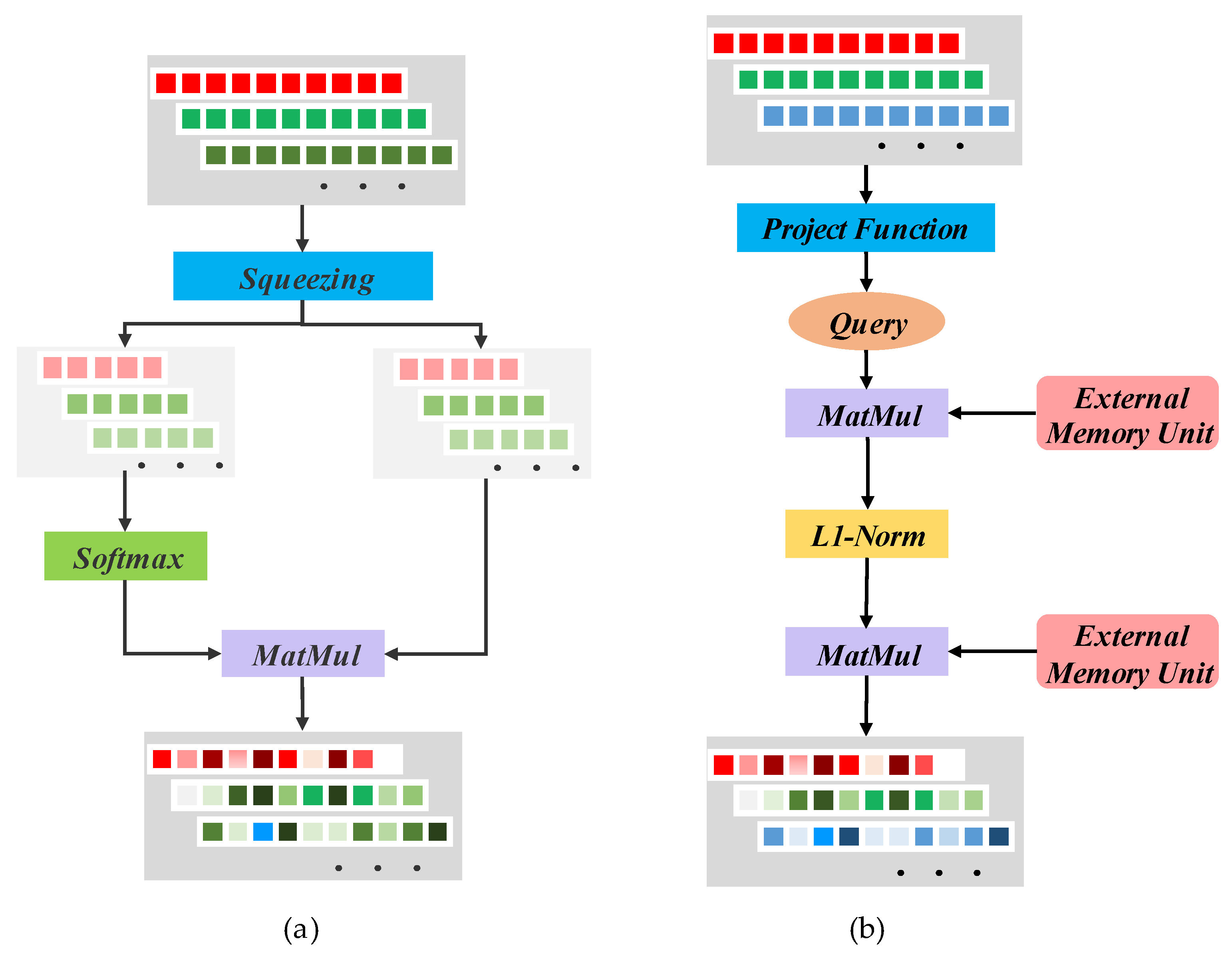
Two self-attention mechanisms, Squeeze-Attention and External-Attention, are proposed for extracting vibration signals. This work will also discuss the affinity of features in the temporal direction that can be obtained, as well as the subject of refining the features by fusing the two methods.

(2)

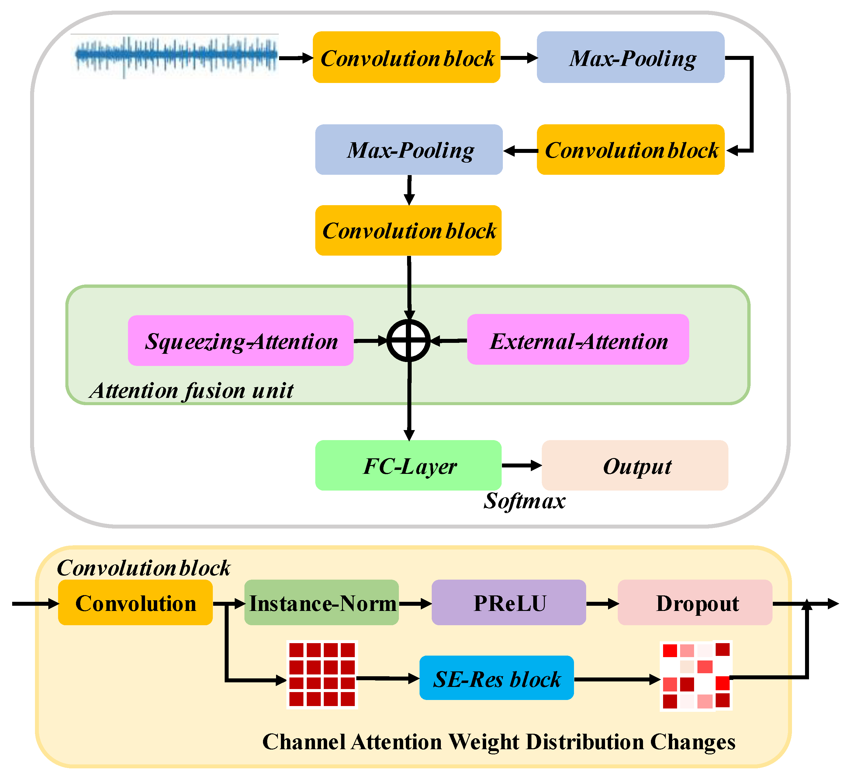
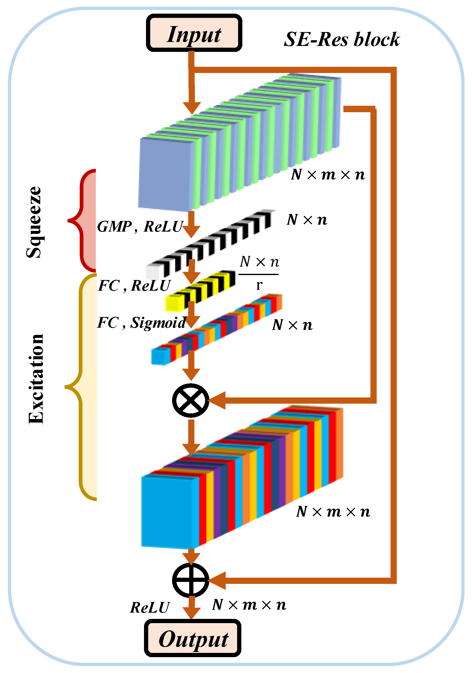
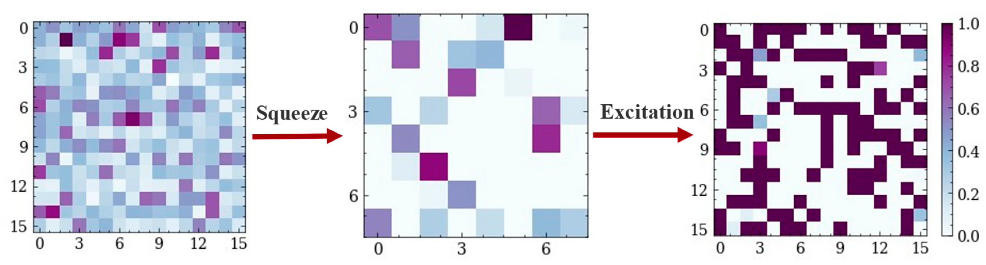
The adaptability of the model to the length of the data is preserved from noise using the convolution block. The feature extraction stage introduces a Squeeze-Excitation one-dimensional residual block (SE-Res block), which removes redundant features contained in the residual connections and captures the nonlinear interactions between channels. This is achieved through the multi-level linkage of attention, focusing on the relationship between feature maps with high fault correlation and channels.

(3)

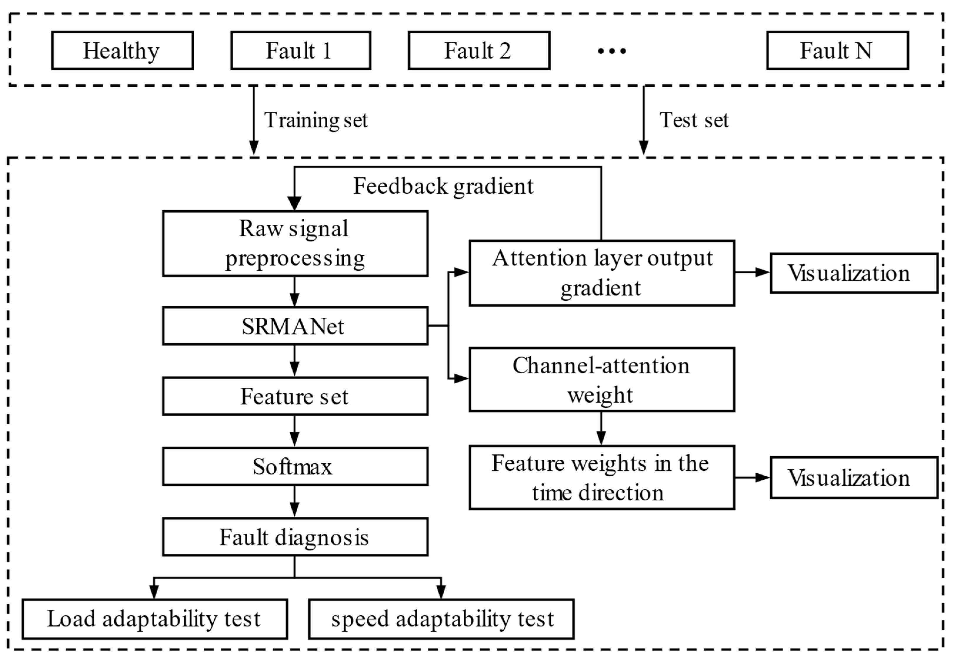
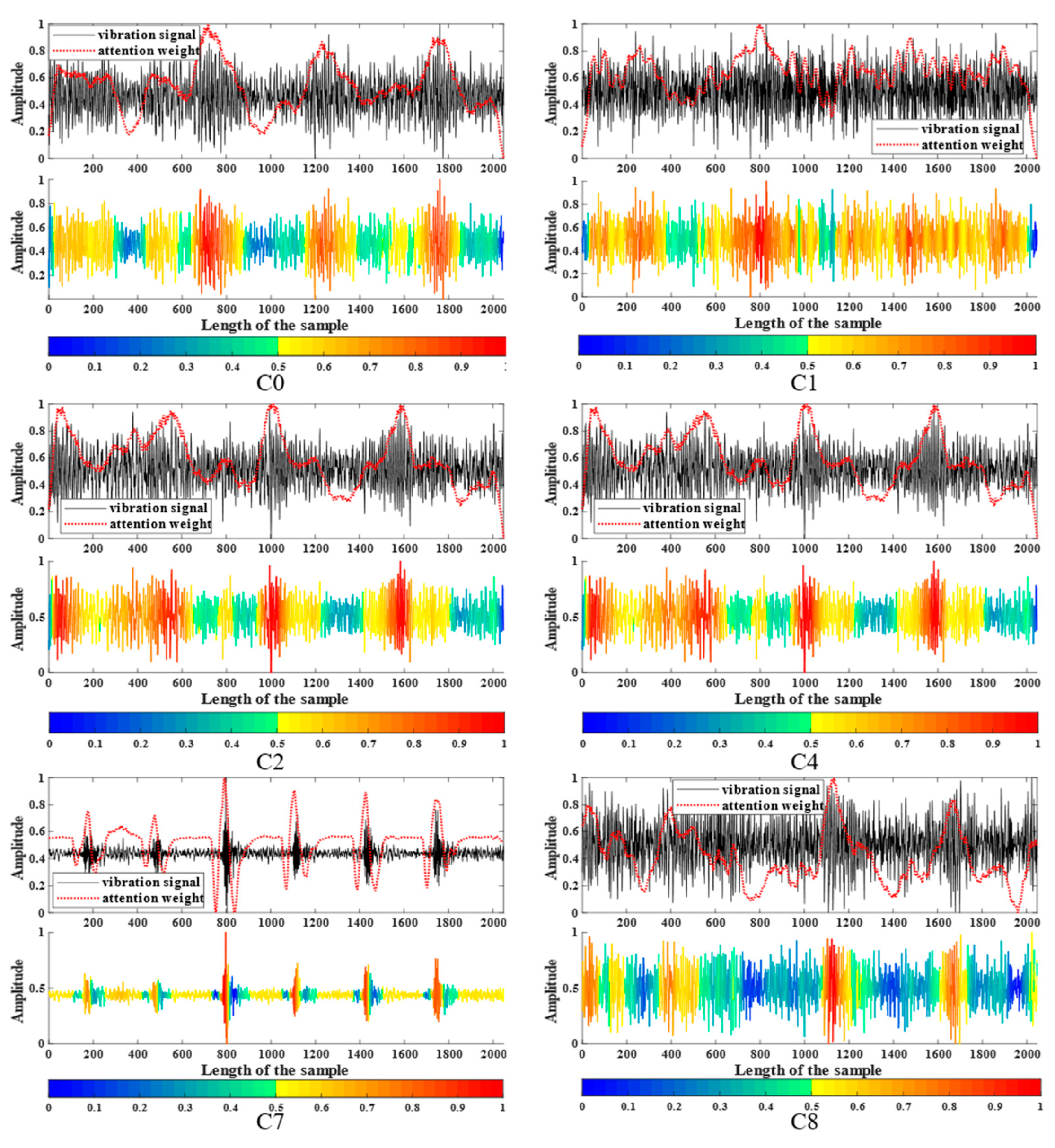
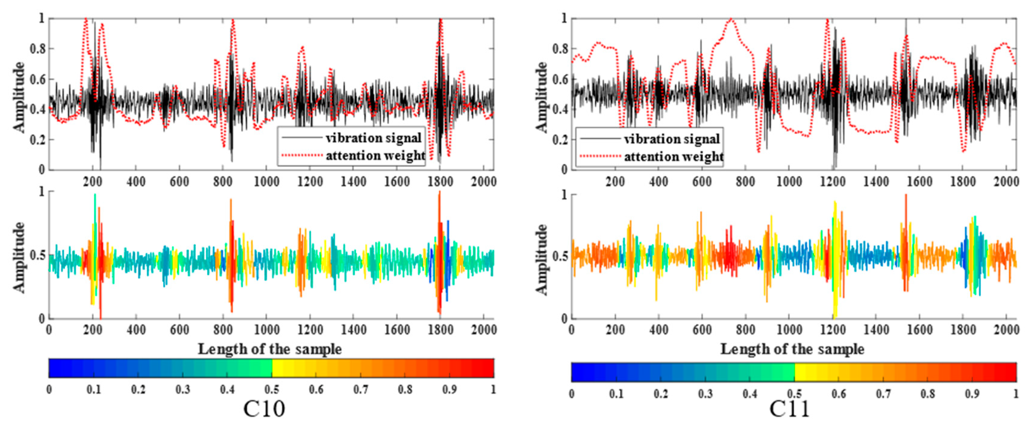
Visualizing arbitrary layer attention weights on input signals using reverse gradients makes the model interpretable. According to the results, it is found that the attention mechanism can assign higher weights to the impulse components of the time-domain signal and lower weights to the fault-independent feature components.

(4)

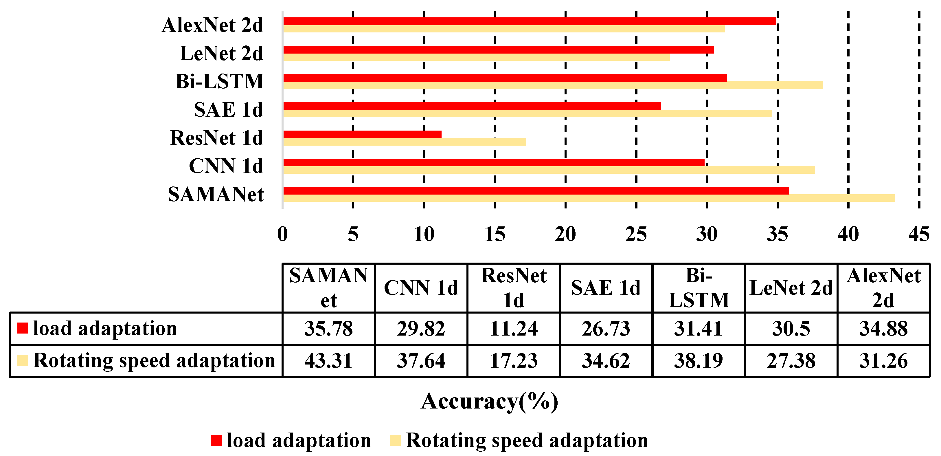
Laboratory planetary gearbox compound faults and single faults of different levels are effectively identified. SRMANet has also been shown in adaptive experiments to be more robust when the load/speed changes.

Section 2 gives details about the SRMANet approach and explores the relevance of CNN to traditional signal processing; Section 3 conducts a validity assessment and interpretability analysis of the proposed method on the planetary gearbox dataset; finally, conclusions and outlooks are provided in Section 4.

2. Stacked Residual Multi-Attention Network Framework

The overall network design of SRMANet is shown in Figure 1, where the convolution block is used to extract representative features of the input signal. The convolution block is composed of a 1D convolution layer, an instance normalization layer, a PReLU layer and a Dropout layer, and residual connection operation is added. Max-Pooling reduces the amount of feature computation and increases the perceptual field of the convolution kernel, embedding squeeze-excitation operations in skip connections to provide high-quality additive features. This process eliminates the problem of model performance degradation due to feature redundancy and learns more sparse features. This training technique highlights the impulse response characteristics in the feature maps.

The attention fusion unit provides an independent attention component for each convolutional kernel output, enhancing the interpretability of SRMANet. The Squeeze-Attention and External-Attention mechanisms are designed to connect directly with the convolutional block. The External-Attention mechanism inserts learnable and shared memory units to enhance the correlation between different features with lower computational complexity. Specific details are provided in the following subsections.

2.1. Convolutional Operations and Interpretability Explored

Vibration signals are typically nonlinear, nonstationary time series. The convolution kernel is able to extract the local features of the signal on a finite time scale, allowing the non-stationary signal to remain locally stable, and is therefore well suited for processing vibration signals. For the input signal, the output of the convolution operation $O_i(c)$ of the $i{\mathrm{th}}^{}$ convolution kernel can be expressed as:

$$O_i(c)=f({\displaystyle \sum x\times k_i(c)}+b_i(c))$$

(1)

× denotes the convolution operation, $c$ is the number of channels, $k$ is the convolution kernel, and $b$ is the bias term.

The essence of a neural network is to learn to approximate a set of functions that map from one feature space to another, a process that is very similar to the properties of the Fourier transform [39]. The Fourier transform (FT) can be viewed as a narrowly defined neural network whose approximation process uses multiple sinusoidal functions to approximate the different intrinsic frequencies of the signal. FT can be expressed as follows:

$$FT[x(t)]={\displaystyle {\int }_{-\infty }^{\infty }x}(t)e^{-i\mathrm{\Omega }t}dt$$

(2)

$x(t)$ is the input signal, $\mathrm{\Omega }=2\pi f$, $f$ is the frequency.

However, FT processes are all univariate transformations, and therefore it is difficult to approximate a mechanical signal, which is a non-stationary signal with time-varying characteristics [40]. The size of the filter corresponds to the scale-transform property in the Fourier transform, and filters of different sizes have different abilities to capture time-domain and frequency-domain features. A time-domain mechanical signal with a complete operating period has fault characteristics that contain both higher-order and lower-order frequency features, which places a requirement on the filter scale.

Higher-order frequency components are generally shorter in duration, while lower-order frequency components are generally longer. A small convolution kernel ensures the ability to extract higher-order frequency features at the expense of the ability to identify lower-order frequency components, while a large convolution kernel does the opposite. Therefore, the DNN design process should include the joint use of filters of different sizes, thus ensuring the time-frequency resolution of the network.

The step length and the number of convolution kernels determine the filter sliding displacement and the number of samples, so the convolution process can be referred to as a multi-granularity scan, i.e., the cyclic overlapping sampling of sample features. The upper layer input information is coarsely granularized using the convolution operator, and the extracted features contain time-shifted and deflated features at multiple scales so that the state information at different moments of the non-stationary time-varying signal can be preserved. This capability—i.e., the ability to localize time and frequency—is not available with many traditional signal analysis methods.

For signal analysis tasks, the engineer expects to complete adequate quantitative and qualitative analysis of the monitoring data. For example, the need to determine which frequencies correspond to a signal at a given moment or which frequencies are contained in a signal at a given moment, and to determine the degree of failure and the location of the failure of a device based on the differences in the components at different moments, coincides with the strengths of DNN. The depth of DNN affects the model complexity and uses kernel functions of different scales to obtain frequency features of different orders, which have stronger approximation and representation capabilities for complex non-stationary signals.

2.2. Instance Normalization Layer

The instantiation normalization process is defined as follows:

$$y=\frac{x-E[x]}{\sqrt{Var[x]+\epsilon }}\times \gamma +\beta$$

(3)

where $E[x]$ is the expectation, and $Var[x]$ is the variance.

To ensure the stability of the values, $\epsilon =1\times {10}^{-5}$ is introduced to avoid the case where the variance is zero. Trainable parameters $\gamma$ and $\beta$ are the scaling factor and shift factor, respectively. The normalization layer can avoid the internal covariate bias problem and improve the convergence speed. This is equivalent to updating the mean and variance of all neurons in the feature map corresponding to a single sample, and then normalizing the neurons. The peak domain range of vibration signals is often different for different operating conditions and different levels of failure. Batch normalization tends to suppress the impulsive nature of signals with lower amplitudes and overemphasizes the violent impulse and apparent disturbances contained in the signal. Unlike batch normalization, the instance normalization process only works on individual data fragments, preserving the private characteristics of each fragment independently. Therefore, the method is more suitable for fault diagnosis training models. The convolution process is simplified to the following representation:

$$Conv(x)=w(x)+b$$

(4)

where $w(x)$ is weight. Convolutional operation is merged with the Instance-Norm process, which is described formally as follows:

$$\begin{array}{ll}IN(Conv(x))& =\frac{w(x)+b-E[x]}{\sqrt{Var[x]+\epsilon }}\times \gamma +\beta \\ & =(\frac{w(x)\times \gamma }{\sqrt{Var[x]+\epsilon }})+(\frac{(b-E[x])\times \gamma }{\sqrt{Var[x]+\epsilon }}+\mathsf{\beta })\\ & {=\mathrm{W}}_{\mathrm{fused}}{\left(\mathrm{x}\right)+\mathrm{B}}_{\mathrm{fused}}\end{array}$$

(5)

2.3. Parametric Rectified Linear Unit (PReLU)

To ensure the nonlinear learning capability of the model, an activation function layer must be added to the DNN. The PReLU operation proceeds as follows:

$$\mathrm{PReLU}\left(x_i\right)=\{\begin{array}{ll}{x}_i\hfill & \mathrm{if} x_i>0\hfill \\ a_i{x}_i\hfill & \mathrm{if} x_i\le 0\hfill \end{array}$$

(6)

where $a_i$ is an updateable parameter.

Compared to the commonly used ReLU, PReLU adds an adaptive slope in the negative direction, allowing the network to take into account both positive and negative responses. This process preserves the low-level features of the signal and fits well with the reciprocal fluctuating nature of the vibration signal.

2.4. Dropout

Dropout is able to randomly freeze neural units with a certain probability during DNN training, which makes each weight update not dependent on a fixed unit [41]. This training technique eliminates the dependencies between neural units and forces the model to learn more robust features.

2.5. SE-Res Block

The structure of the proposed SE-Res block for a one-dimensional vibration signal is shown in Figure 2, with the feature map at the input. $\mathrm{N}$ denotes batch size, $\mathrm{m}$ is the number of feature map dimensions and $n$ is the number of channels. The module’s dynamic selection process for channels is divided into two parts: squeezing and excitation. Referring to SENet [30], where the squeezing operation is implemented by a global average pooling layer (GMP), the process is able to aggregate feature maps to form a global distribution of embedded channel-wise features. The squeezing process is defined as follows:

$$z_n=F_{sq}(u_n)=\frac{1}{L}{\displaystyle \sum _{i=1}^L{u}_n}[i]$$

(7)

$u_n\in {ℝ}^{m\times n}$ denotes the feature map of the input, and $L$ is the length of the feature map for a single channel.

The excitation operation is implemented through the fully connected layer (FC) and is designed to capture the dependencies between channels. This relationship is not a simple one-hot vector pattern, but is nonlinear or nonreciprocal. The end is implemented by the Sigmoid activation function for the adaptive acquisition of modulation weights. The introduction of $r$ in the figure adds a gating mechanism to the excitation process, reducing the complexity and enhancing the robustness of the residual module. The process is defined as follows:

$$w=F_{ex}(z,W)=\sigma (g(z,W))=\sigma \left(W_2\sigma \left(W_{1}z\right)\right)$$

(8)

$${\tilde{u}}_n=w_n\times u_n$$

(9)

where $W_1\in {ℝ}^{\frac{n}{r}\times n}$ and $W_2\in {ℝ}^{\frac{n}{r}\times n}$ represent the weight matrices of the two FC. In this article r was set to 4. $\sigma$ is the ReLU function, ${\tilde{u}}_n$ is the result of rescaling the Sigmoid activation function.

The above process is capable of adaptively assigning weights to different feature maps and explicitly constructing interdependencies between channels by weighting. The pattern integration of the dynamic channel selection process and the residual connection allows for obtaining additive features with lower redundancy and reinforcing feature maps with higher correlation. The SE-Res block can finally be represented as:

$$y=u_n+w\times u_n$$

(10)

2.6. Attention Fusion Unit

Inspired by [42], for time series analysis, this study proposes two temporally oriented attention mechanisms, Squeeze-Attention and External-Attention. The specific process is shown in Figure 3, and both methods ensure that the inputs and outputs are consistent, in line with the generic properties of the model. Squeeze-Attention (Figure 3a) is a simplified version of self-attention. “Squeezing” and “Expanding” refer to the linear down-sampling transformation of the input feature map and the up-sampling of the attention output matrix, respectively. It can be found that Squeeze-Attention is able to add a gating mechanism in the time direction at the input, which can ensure that the input and output remain consistent. The method can be expressed as follows:

$$\begin{array}{l}soft\max \left(x_i\right)=\frac{e^{x_i}}{{\displaystyle {\sum }_j{e}^{x_j}}}\\ A={(\alpha )}_{i,j}=soft\max \left(F_{tr}{(u_n)}_1\right)\\ F_{out}=F_{\exp }(A\times F_{tr}{(u_n)}_2)\end{array}$$

(11)

where ${(\alpha )}_{i,j}$ denotes the affinity matrix in the time direction, $F_{tr}$ denotes a linear transformation, and $F_{\exp }$ is the up-sampling process.

However, Squeeze-Attention’s focus is on the filtering results of a single filter in the time direction. To this end, this study incorporates the advantages of External-Attention (Figure 3b). External-Attention introduces learnable external memory units capable of expanding attention to all channels and retaining previous training memories. L1-Norm eliminates scale sensitivity of features. The method can be expressed as follows:

$$\begin{array}{l}{\mathrm{F}=\mathrm{f}}_{\mathrm{proj}}{(\mathrm{u}}_{\mathrm{n}})\\ \mathrm{A}=\mathrm{Norm}\left({\mathrm{FM}}_{\mathrm{k}}^{\mathrm{T}}\right)\\ {\mathrm{F}}_{\mathrm{out} }{=\mathrm{AM}}_{\mathrm{v}}\end{array}$$

(12)

where $\mathrm{F}\in {ℝ}^{s\times n}$ is the feature map after linear projection, ${\mathrm{M}}_{\mathrm{k}}\in {ℝ}^{s\times n}$ and ${\mathrm{M}}_{\mathrm{v}}\in {ℝ}^{s\times n}$ are external memory units. s is the hyperparameter of the memory unit, capable of controlling the memory unit size. To ensure consistent input and output, the same up-sampling strategy needs to be added at the end of the method. The complete training process of the model is summarized in Algorithm 1. The methodology flow chart is provided in Figure 4.

Algorithm 1: SRMANet training process

Input:$n$ single channel training data of any cut length $X={\left\{x^i\right\}}_{i=1}^n$, corresponding labels $Y={\left\{y^i\right\}}_{i=1}^n$ and position set of visualization layer $p\subseteq \{1,2\cdots \max \{L\left\}\right\}$, where $L$ indicates the model depth Parameters: learning rate $\gamma$, epoch $T_{\max }$, SRMANet model parameter ${\theta }_M$, class number K, Gating ratio $r$ in Equation (8) and hyperparameter of the memory unit $s$ in Equation (12) Output: SRMANet model M and Gradient set ofvisualization layer $\{▽f\}$ 1: Initialize ${\theta }_M$ and shuffle the train set $\{X,Y\}$ 2: for $t=1,2\dots \dots T_{\max }$ do 3:    Calculate cross entropy loss $los{s}_{clf}={\{L({\theta }_M),x_k\}}_{k=1}^K$ 4:    Calculate $P_{th}$ model gradient $grad\{{\theta }_M,X,p\}=\{▽f\}=\{\partial {\theta }_M^p/\partial {\left\{x^i\right\}}_{i=1}^n\}$ 5:    update ${\theta }_M={\theta }_M+\gamma ▽los{s}_{clf}$ 6:    if $t\%10==0$ then 7:    return model parameter ${\theta }_M$ and $\{▽f\}$ 8:    end if 9: end for

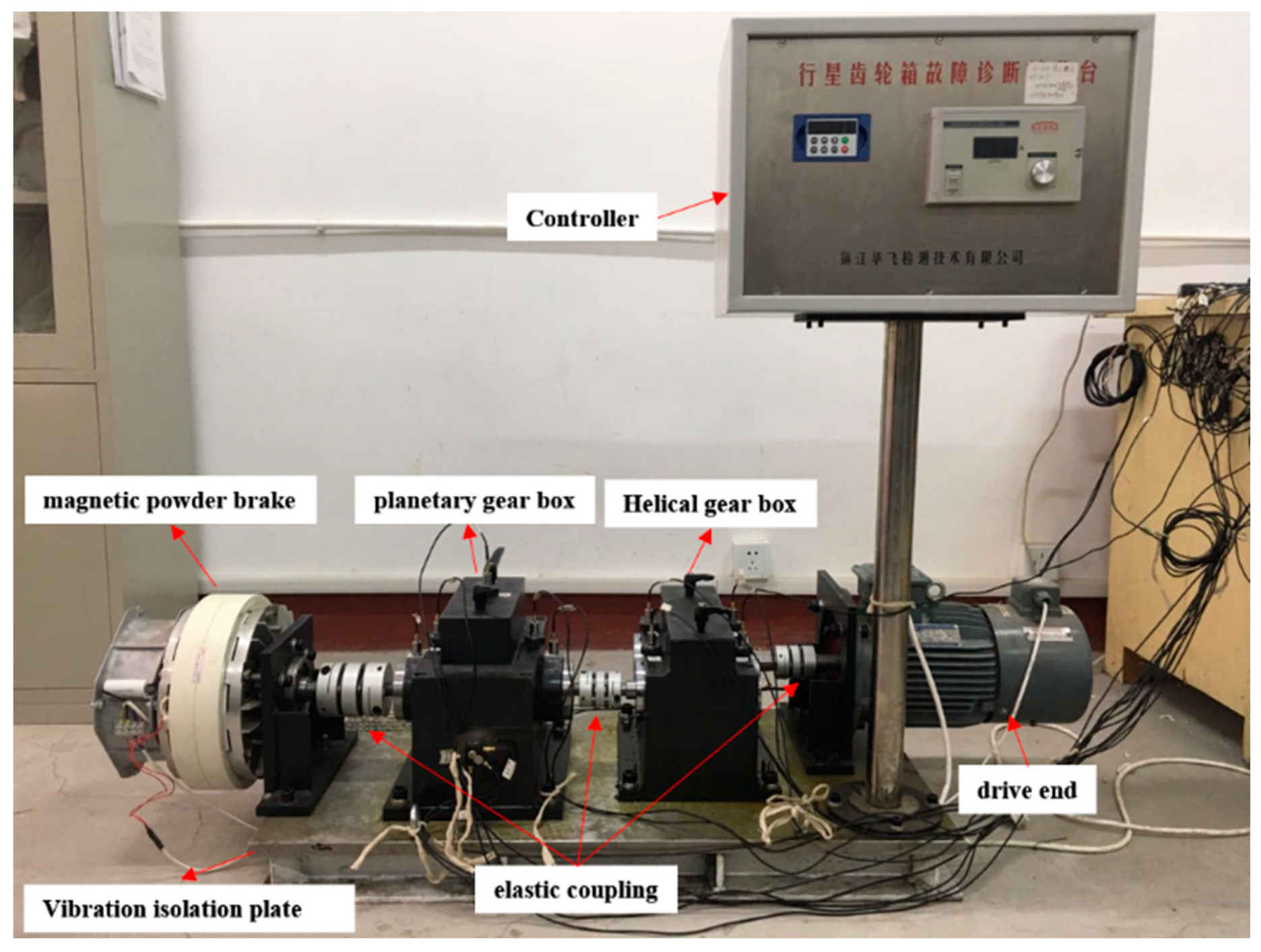
3. Experimental Verification

To verify the performance of SRMANet in fault recognition, a planetary gearbox dataset that was measured in the laboratory was used for fault diagnosis experiments. In this study, all experiments were performed using Tensorflow 2.5.0 on python 3.8.3. The computer has a Core i7-8750 CPU@2.20 GHz processor and works on a Windows 64-bit operating system. To improve the training speed, a GPU (GTX1660Ti) with 6 GB memory is added.

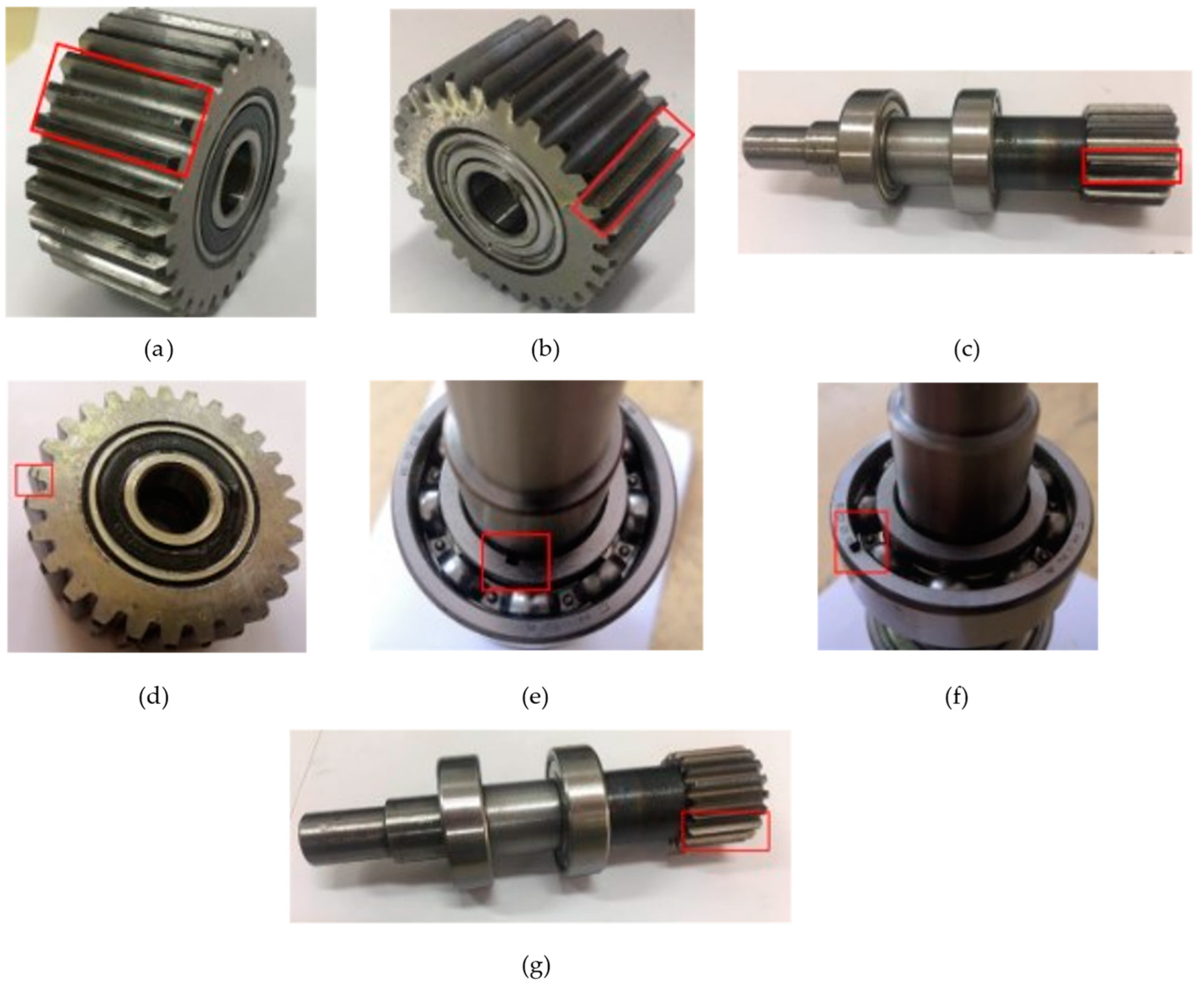
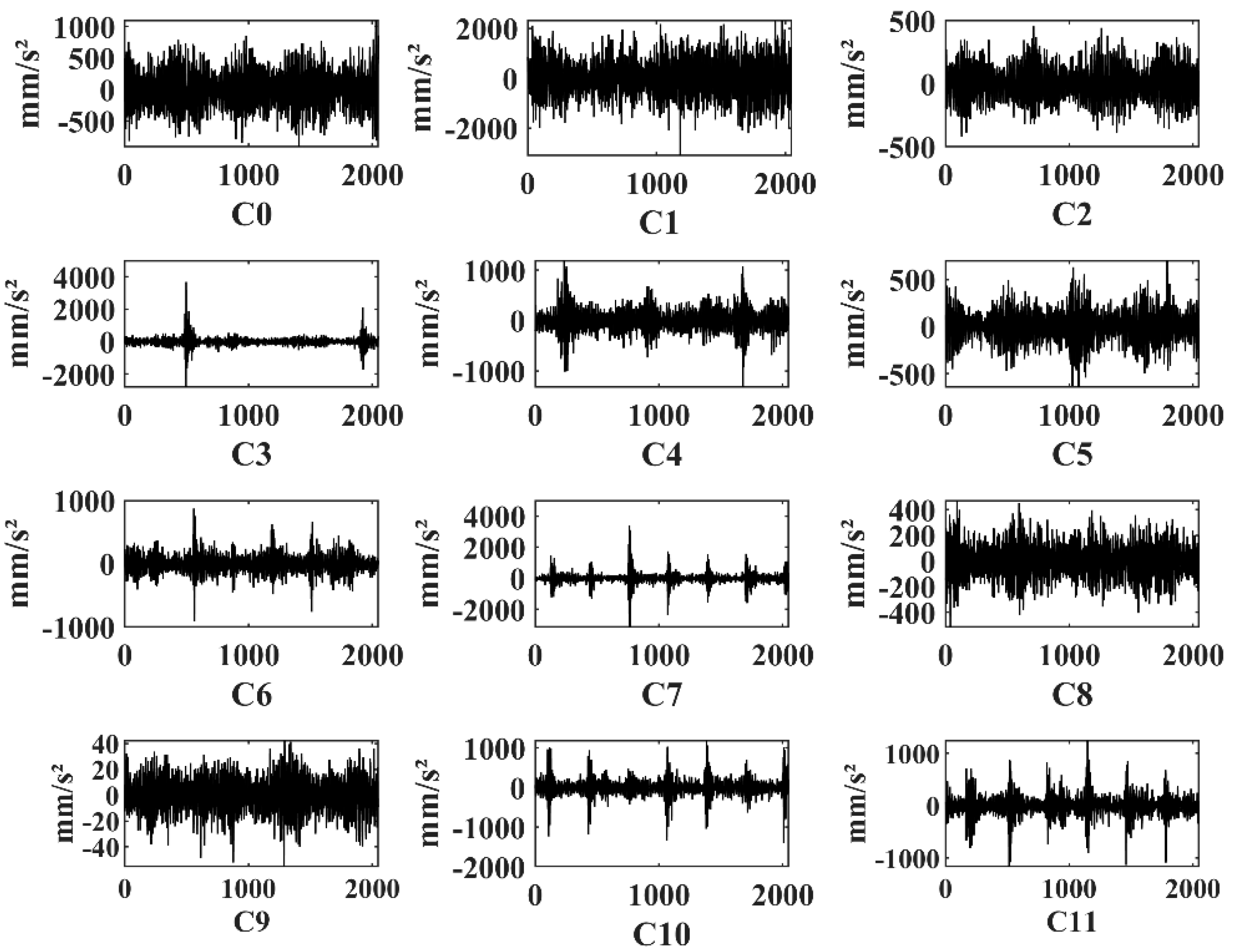
3.1. Description of the Dataset

The planetary gearbox HFXZ-I dataset from the laboratory was applied to the study of fault diagnosis methods in this paper. The experimental platform is shown in Figure 5 and mainly consists of a variable speed drive motor, a coupling, a helical gearbox, a planetary gearbox, a magnetic powder brake, a variable speed drive controller and a load controller. The relevant base parameters are shown in

Table 1. Basic parameters of the planetary gearbox.

Parameters	Ring Gear Teeth (Nr)	Planetary Gear Teeth (Np)	Sun Gear Teeth (Ns)	Planet Gears	Type of Planetary Gear Box
numbers	72	27	18	3	single

. The data source selects the vibration signal measured by the acceleration sensor mounted on top of the planetary gearbox. The vibration signal was sampled continuously for one minute at three motor speeds (approx. 1200 r/min, 900 r/min, 600 r/min) and three loads (1 A, 0.5 A, 0.3 A) according to the 10,240 Hz sampling frequency.

This experiment starts from the planetary gearbox system, which contains typical failures common inside a planetary gearbox, including gear pitting, gear wear, sun gear broken teeth, sun gear wear, gear cracks, inner race defects, and outer race defects. The details of the faults are shown in Figure 6. To further enhance the adaptability of the method to the degree of failure, the experiments were carried out for each of the different failure modes to further test the generality of the method as well as its ability to determine the level of failure. Experiments were performed thirty-six times, corresponding to the twelve types of failures under three load and speed operating conditions.

It is worth mentioning that this experimental dataset mixes single and compound faults and single faults of different fault levels, which can further demonstrate the decoupling capability of the method for faults and the generality of the extracted features. Another advantage that the model proposed in this method possesses is that the input data are variable in length. For this reason, data of different cut lengths are provided in the data pre-processing stage. The proportion of the training set is 30% of the total data. The details of the experimentally acquired data are shown in

Table 2. Details about the dataset.

Pattern Label	Gearbox	Rotating Speed (Hz) + Load (A)	Length of Samples	Training Ratio
C0	Normal	40 + 1/30 + 0.5/20 + 0.3	1024/2048/4096	30%
C1	Gear pitting	40 + 1/30 + 0.5/20 + 0.3	1024/2048/4096	30%
C2	Gear crack	40 + 1/30 + 0.5/20 + 0.3	1024/2048/4096	30%
C3	Gear wear (level 1)	40 + 1/30 + 0.5/20 + 0.3	1024/2048/4096	30%
C4	Gear wear (level 2)	40 + 1/30 + 0.5/20 + 0.3	1024/2048/4096	30%
C5	Gear wear (level 3)	40 + 1/30 + 0.5/20 + 0.3	1024/2048/4096	30%
C6	Sun gear broken teeth (level 1)	40 + 1/30 + 0.5/20 + 0.3	1024/2048/4096	30%
C7	Sun gear broken teeth (level 2)	40 + 1/30 + 0.5/20 + 0.3	1024/2048/4096	30%
C8	Inner race defect	40 + 1/30 + 0.5/20 + 0.3	1024/2048/4096	30%
C9	Outer race defect	40 + 1/30 + 0.5/20 + 0.3	1024/2048/4096	30%
C10	Sun gear wear + C1	40 + 1/30 + 0.5/20 + 0.3	1024/2048/4096	30%
C11	Sun gear wear + C4	40 + 1/30 + 0.5/20 + 0.3	1024/2048/4096	30%

. The vibration signals corresponding to different pattern labels are shown in Figure 7. It should be emphasized that the signal amplifier multipliers in the experiments are different for different operating conditions, and thus the vibration acceleration values are in different ranges. Data is normalized when used.

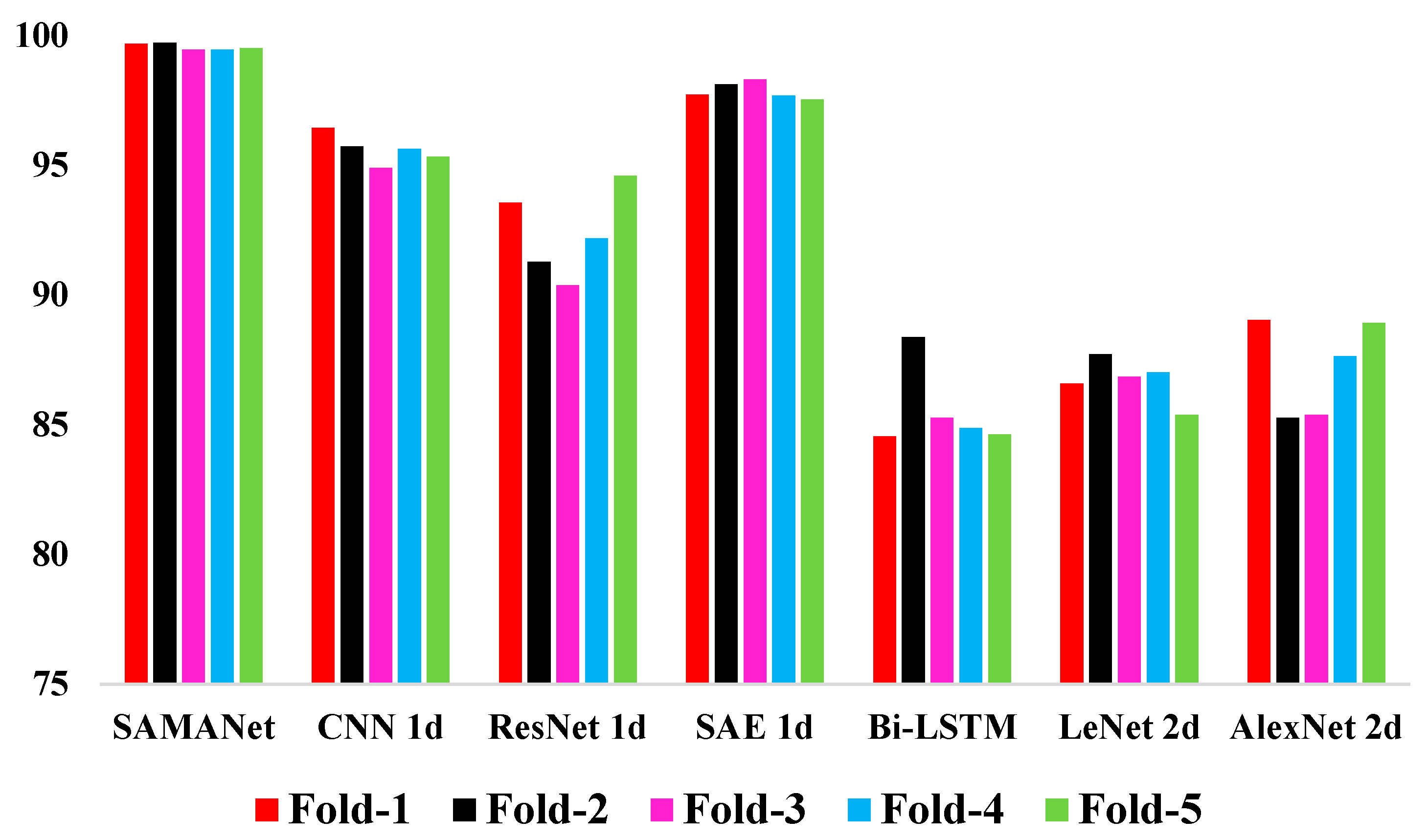
3.2. Experimental Results and Analysis

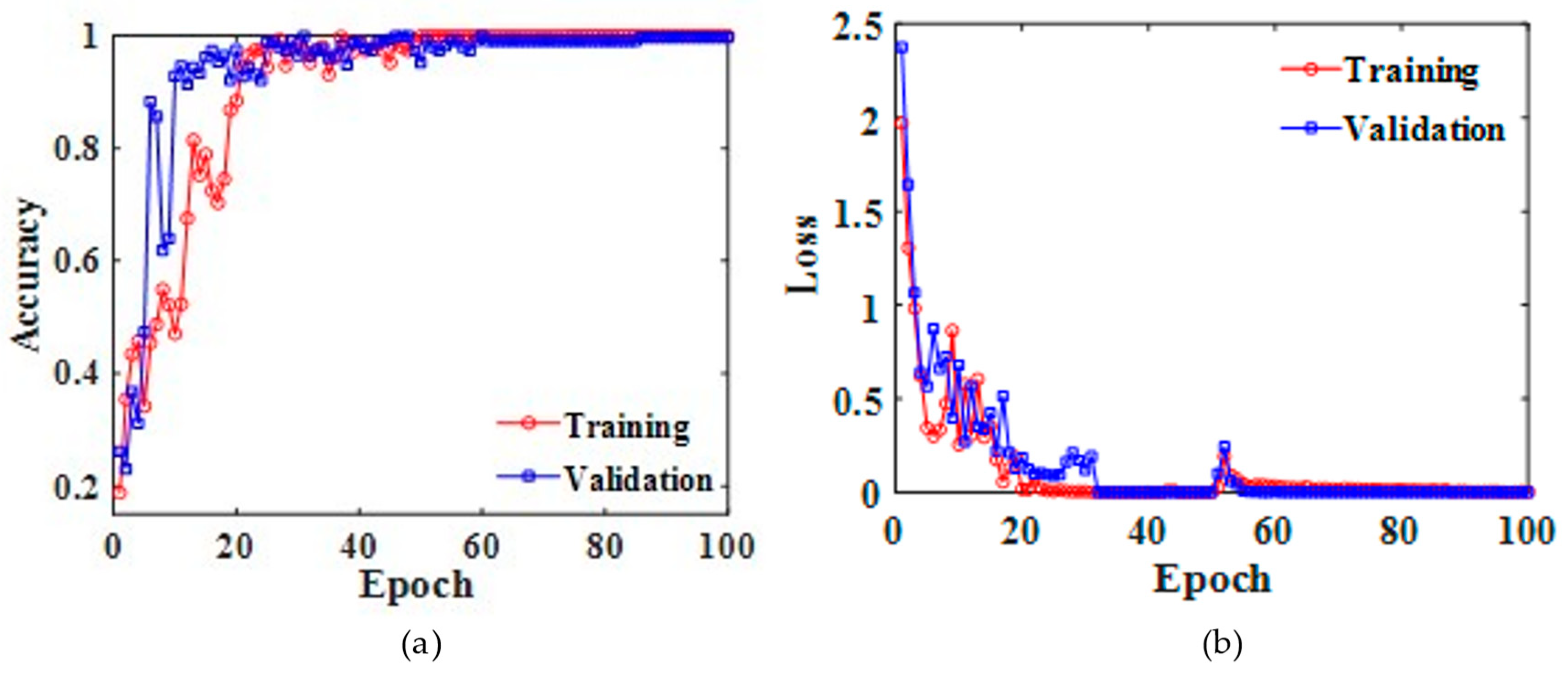
3.2.1. Parameter Settings and Training Process

According to the Figure 1 in Section 2, the network structure and parameter setup of SRMANet are presented in

Table 3. Structure parameters and hyper-parameters setup of SRMANet.

Structure	Parameters	Outputs Size
Input	vibration signal	[1024 × 1]/[2048 × 1]/[4096 × 1]
Convolution block 1	F = 128; KS = 5; S = 1; DR = 0.5; r = 4	[128@1024 × 1]/[128@2048 × 1]/[128@4096 × 1]
Max-Pooling	Pool size = 2	[128@512 × 1]/[128@1024 × 1]/[128@2048 × 1]
Convolution block 2	F = 256; KS = 11; S = 1; DR = 0.5; r = 4	[256@512 × 1]/[256@1024 × 1]/[256@2048 × 1]
Max-Pooling	Pool size = 2	[256@256 × 1]/[256@512 × 1]/[256@1024 × 1]
Convolution block 2	F = 512; KS = 11; S = 1; DR = 0.5; r = 4	[512@256 × 1]/ [512@512 × 1]/[512@1024 × 1]
Attention fusion unit	SR = 0.5; GS = 64	[256@256 × 1]/[256@512 × 1]/[256@1024 × 1]
FC (linear Projection)	Hidden Nodes = 32; activation = Sigmoid	[32@256 × 1]/[32@512 × 1]/[32@1024 × 1]
Flatten	None	8192/16384/24576
FC	Hidden Nodes = 12; activation = Softmax	[12 × 1]
hyper-parameters	Loss: cross entropy loss; Batch size = 16; Validation ratio = 0.1; Optimizer: Adam; Learning rate = 0.0003

, where F represents the number of filters; KS represents filter width; DR represents the dropout rate; and R represents the gating size in the SE-Res block. SR is the compression ratio of Squeeze-Attention; GS is the gating size of External-Attention, which controls the computational complexity. The [32@256 × 1] denotes the 32 feature maps of size 256 × 1. It should be pointed out that the SE-Res block enhances the training stability, which is used together with dropout to reduce the risk of overfitting.

The data with 40 Hz speed, 1 A load and 2048 sample length were selected as the benchmark dataset and the following part of the study was carried out using this benchmark dataset. The training process of SRMANet is presented in Figure 8. We found that SRMANet converges quite rapidly. After testing, it was found that SRMANet could identify almost all samples at an epoch of about 60 times. This illustrated SRMANet’s capacity to identify universal features from vibration signals.

3.2.2. Visualization Analysis of SE-Res Block

DNNs have always been subject to the stereotype that they are unreliable in the field of device health management because their internal training process is not visible to the users. In this section, we focus on visualizing the Squeeze-Excitation operation in the SE-Res block to show the effectiveness of SRMANet.

The intermediate process is visualized with planetary gearbox data, as shown in Figure 9. The product of the horizontal and vertical coordinates plus one is the corresponding number of channels, i.e., the three intermediate layers in Figure 9 contain 256, 64 and 25 channels, respectively. Obviously, the convolution kernel extracts a set of feature maps corresponding to the more haphazard distribution of channel attention weights. Each channel is only concerned with local features at each time step of the convolution kernel, lacking an understanding of global information and thus containing more redundant information.

After the Squeeze-Excitation operation, the distribution of weights among different feature maps is more discrete. A large number of fault-independent feature maps are adaptively and dynamically eliminated, preserving the information dependencies between different channels. After the excitation operation, the relationship between channels has stronger sparsity and redundant information is effectively removed.

3.2.3. Attention Fusion Unit Visualization

Based on the gradient at the output of the attention fusion unit, which is fed back to the original signal, the attention weights corresponding to the signal can be obtained. Figure 10 shows SRMANet’s attention weights for partial single-fault conditions. Figure 11 visualizes the attention weights for compound fault conditions.

The color bars at the bottom of the figure show the colors corresponding to the different attention weight sizes after normalization. A similar approach was used in [37] to visualize the bearings in question. This study is somewhat different, however, as the planetary gearbox signal is more complex and has more internal disturbances. To better illustrate the representative features learned by SRMANet, the output features of the attention fusion unit are further extended and refined in this study.

According to the results of this study, SRMANet’s ability to learn the features and characteristics of what we think of as a rule of thumb is not consistent. As in the case of planetary gear wear (Figure 10—C4) and sun wheel broken tooth failure (Figure 10—C7), SRMANet does not assign a high learning weight to some of the large impulses. Most of the segments of gear wear faults were assigned high weights. Moreover, by comparing different degrees of sun wheel broken tooth faults (Figure 10—C7,C8), it can be found that SRMANet is relatively weak at capturing weak fault features. Finally, for compound faults, SRMANet is able to effectively localize faults to the impulse characteristics in the time domain.

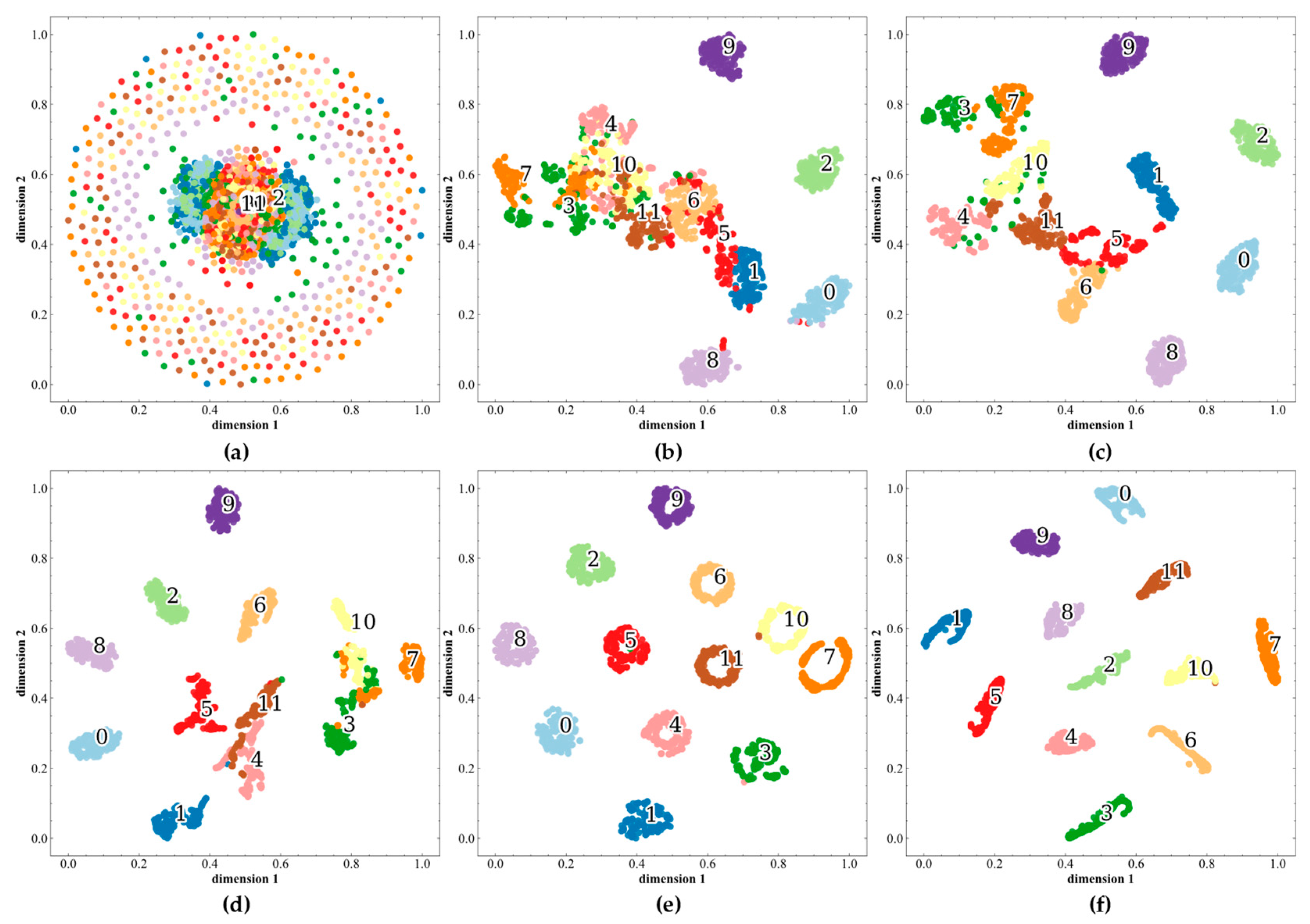
3.2.4. Network Middle Layer Visualization

To further validate SRMANet’s excellent ability to recognize signals containing complex components and to explain SRMANet’s learning process, this subsection presents the visualization of SRMANet’s middle layer. Figure 12 shows the distribution of features in two dimensions for the different intermediate layers. The tensor features of the interlayer output are projected onto the low-dimensional space via t-distributed random neighborhood embedding (t-SNE). The figure contains the numbers from 0 to 11, corresponding to the different operating conditions from C0 to C11 of the planetary gearbox.

Obviously, the distribution of features of the original signal is highly aggregated. As the SRMANet network deepens, the samples of different working conditions are gradually separated and the distance of samples of the same working condition keeps decreasing. When the final layer of SRMANet is reached, the twelve types of operating conditions of the planetary gearbox can be precisely identified.

3.3. Discussion

In this section, SRMANet is compared with other deep learning methods to demonstrate its superiority in learning representative features. To ensure the validity of the results, the validation experiments were compared using the code open-source benchmark model [43].

The models compared include one-dimensional convolutional neural networks (CNN 1d), one-dimensional residual neural networks (ResNet 1d), one-dimensional stacked self-encoders (SAE 1d), bi-directional long and short-term memory networks (Bi-LSTM), and the classic LeNet and AlexNet. The two-dimensional DNN model uses time-domain images as validation data.

Figure 13 shows the recognition performance of different DNN models based on five-fold cross-validation.

Table 4. Fold-1 accuracy (%) of different DNN models.

	SRMANet	CNN 1d	ResNet 1d	SAE 1d	Bi-LSTM	Lenet 2d	Alexnet 2d
C0	99.98	97.53	94.76	98.71	79.93	81.37	90.42
C1	99.70	98.41	96.13	99.93	84.71	84.72	90.75
C2	99.03	97.16	95.28	98.32	91.77	94.37	88.71
C3	99.64	94.32	93.26	96.52	92.19	87.50	84.37
C4	99.50	95.01	92.50	94.37	82.73	92.71	89.22
C5	99.49	96.71	91.59	95.92	82.37	85.37	80.07
C6	100.00	96.47	97.12	97.87	78.56	82.54	83.94
C7	99.90	94.73	94.93	98.12	74.37	93.78	94.36
C8	99.70	95.32	93.42	98.37	88.70	78.54	92.51
C9	99.67	96.50	89.71	99.24	78.92	77.32	85.63
C10	99.46	96.31	91.73	97.52	89.75	88.64	93.65
C11	100.00	98.72	92.14	99.80	90.42	92.21	94.77
Average	99.67	96.43	93.55	97.72	84.54	86.59	89.03

shows the accuracy of all DNN methods in Fold-1, where SRMANet achieves an impressive 100% accuracy in the C6 and C11 recognition tasks. It is easy to see that SRMANet performs better in the analysis of complex data, such as those related to planetary gearboxes.

Datasets with different sample lengths are selected separately for validation without changing the model structure and parameters. According to

Table 5. Average accuracy (%) of SRMANet for different conditions.

Rotating Speed (Hz) + Load (A)	Sample Length 1024	Sample Length 2048	Sample Length 4096
40 Hz + 1 A	98.92 ± 0.42	99.67 ± 0.07	99.92 ± 0.01
30 Hz + 0.5 A	99.14 ± 0.24	99.84 ± 0.11	99.91 ± 0.03
20 Hz + 0.3 A	98.64 ± 0.17	99.86 ± 0.02	99.95 ± 0.01

, the sensitivity of SRMANet to changes in sample lengths is found to be low, indicating that it is able to perform well in a number of generic fault diagnosis tasks.

On the other hand, the accuracy of validation under the same dataset still lacks reliability, so tests of model generalization capabilities need to be carried out. The generalization ability of the model is still one of the problems that are difficult to overcome at the moment, and transfer learning provides us with ideas. However, it was found through validation that this type of transfer method only performs well with fewer working conditions and distinct data characteristics. Therefore, transfer learning should be enhanced from another perspective, i.e., by designing models that extract representative features

Learning representative features requires models with stronger generalization capabilities and adaptability to secondary factors. Load and speed, as typical secondary factors, are very likely to interfere with the diagnosis results in fault diagnosis tasks, which is one of the reasons why transfer learning is currently a hot topic. Here we mainly consider the robustness of the model. Large differences were found in the distribution of the data for the same fault at different speeds and loads.

We performed a load adaptation analysis (

Table 6. Load adaptability test results.

Length/Rotating Speed	1 A→0.5 A	1 A→0.3 A	0.5 A→0.3 A	0.3 A→0.5 A	0.3 A→1 A	0.5 A→1 A	Average
1024/30 Hz	44.71	37.63	34.26	32.61	29.71	27.24	34.36
2048/30 Hz	46.27	39.92	34.18	34.50	31.24	25.32	35.24
4096/30 Hz	49.10	40.33	38.77	36.67	32.22	29.36	37.74
Average	46.69	39.29	35.74	34.59	31.06	27.31	35.78

) and a speed adaptation analysis (

Table 7. Rotating speed adaptability test results.

Length/Load	40 Hz→30 Hz	40 Hz→20 Hz	30 Hz→20 Hz	20 Hz→30 Hz	20 Hz→40 Hz	30 Hz→40 Hz	Average
1024/1 A	41.37	39.28	46.36	38.14	33.44	36.10	39.12
2048/1 A	48.93	44.88	51.21	39.62	43.27	39.19	44.52
4096/1 A	54.31	49.37	42.53	43.20	45.12	43.18	46.29
Average	48.20	44.51	46.70	40.32	40.61	39.49	43.31

) by means of a model-based transfer learning approach. The arrows indicate the transfer process of the model between different working conditions. It can be seen that the performance of SRMANet decreased significantly under changing loads and speeds, which is due to the change in data distribution.

Figure 14 compares the results against those of other models, and shows that the adaptability of the proposed SRMANet model still maintains a slight advantage. This indicates that SRMANet as a feature extractor is more representative and general in the features it obtains.

4. Conclusions

In this paper, SRMANet, a fault diagnosis model incorporating multiple attention mechanisms, is proposed, and can visualize the training process and improve model interpretability. The model proved to be effective in identifying compound faults in planetary gearboxes. The results of this paper are summarized as: (1) component changes to the standard CNN model provide physical meaning while enhancing the ability of the model to extract representative features; (2) the SE-Res block is designed so that the feature channels being weighted are more sparse; (3) Squeeze-Attention and External-Attention are proposed, and the gradient of their fused output is fed back to the original signal, further demonstrating the ability of the attention mechanism to capture impulse components and fault-related components. The experimental results show that SRMANet is interpretable and maintains a good level of robustness and self-adaptability when the load and speed change.

References

1. Elbi, M.D.; Kizilkaya, A. Multicomponent signal analysis: Interwoven Fourier decomposition method. Digit. Signal Processing 2020, 104, 102771. [Google Scholar] [CrossRef]
2. Cheng, J.; Yang, Y.; Shao, H.; Pan, H.; Zheng, J.; Cheng, J. Enhanced periodic mode decomposition and its application to composite fault diagnosis of rolling bearings. ISA Trans. 2022, 125, 474–491. [Google Scholar] [CrossRef] [PubMed]
3. Zhou, W.; Feng, Z.; Xu, Y.F.; Wang, X.; Lv, H. Empirical Fourier Decomposition: An Accurate Adaptive Signal Decomposition Method. arXiv 2020, arXiv:2009.08047. [Google Scholar]
4. Liu, Y.; Han, J.; Zhao, S.; Meng, Q.; Shi, T.; Ma, H. Study on the Dynamic Problems of Double-Disk Rotor System Supported by Deep Groove Ball Bearing. Shock. Vib. 2019, 2019, 8120569. [Google Scholar] [CrossRef]
5. Luo, Z.; Wang, J.; Tang, R.; Wang, D. Research on vibration performance of the nonlinear combined support-flexible rotor system. Nonlinear Dyn. 2019, 98, 113–128. [Google Scholar] [CrossRef]
6. Singh, P.; Joshi, S.D.; Patney, R.K.; Saha, K. The Fourier decomposition method for nonlinear and non-stationary time series analysis. Proc. R. Soc. A 2017, 473, 20160871. [Google Scholar] [CrossRef] [Green Version]
7. Wang, B.; Lei, Y.; Li, N.; Yan, T. Deep separable convolutional network for remaining useful life prediction of machinery. Mech. Syst. Signal Processing 2019, 134, 106330. [Google Scholar] [CrossRef]
8. Luo, J.; Huang, J.; Li, H. A Case study of conditional deep convolutional generative adversarial networks in machine fault diagnosis. J. Intell. Manuf. 2021, 32, 407–425. [Google Scholar] [CrossRef]
9. Zhang, Y.; Li, X.; Gao, L.; Chen, W.; Li, P. Ensemble deep contractive auto-encoders for intelligent fault diagnosis of machines under noisy environment. Knowl. -Based Syst. 2020, 196, 105764. [Google Scholar] [CrossRef]
10. Xiang, S.; Qin, Y.; Zhu, C.; Wang, Y.; Chen, H. Long short-term memory neural network with weight amplification and its application into gear remaining useful life prediction. Eng. Appl. Artif. Intell. 2020, 91, 103587. [Google Scholar] [CrossRef]
11. Jin, Y.; Qin, C.; Huang, Y.; Liu, C. Actual bearing compound fault diagnosis based on active learning and decoupling attentional residual network. Measurement 2021, 173, 108500. [Google Scholar] [CrossRef]
12. Ma, P.; Zhang, H.; Fan, W.; Wang, C. A diagnosis framework based on domain adaptation for bearing fault diagnosis across diverse domains. ISA Trans. 2020, 99, 465–478. [Google Scholar] [CrossRef] [PubMed]
13. He, K.; Zhang, X.; Ren, S.; Sun, J. Deep Residual Learning for Image Recognition. In Proceedings of the 2016 IEEE Conference on Computer Vision and Pattern Recognition (CVPR), Las Vegas, NV, USA, 27–30 June 2016; pp. 770–778. [Google Scholar] [CrossRef] [Green Version]
14. Chen, Y.; Peng, G.; Xie, C.; Zhang, W.; Li, C.; Liu, S. ACDIN: Bridging the gap between artificial and real bearing damages for bearing fault diagnosis. Neurocomputing 2018, 294, 61–71. [Google Scholar] [CrossRef]
15. Ma, S.; Chu, F.; Han, Q. Deep residual learning with demodulated time-frequency features for fault diagnosis of planetary gearbox under nonstationary running conditions. Mech. Syst. Signal Processing 2019, 127, 190–201. [Google Scholar] [CrossRef]
16. Zhang, W.; Li, X.; Ding, Q. Deep residual learning-based fault diagnosis method for rotating machinery. ISA Trans. 2019, 95, 295–305. [Google Scholar] [CrossRef]
17. Zhao, M.; Zhong, S.; Fu, X.; Tang, B.; Dong, S.; Pecht, M. Deep Residual Networks With Adaptively Parametric Rectifier Linear Units for Fault Diagnosis. IEEE Trans. Ind. Electron. 2021, 68, 2587–2597. [Google Scholar] [CrossRef]
18. Zhao, M.; Tang, B.; Deng, L.; Pecht, M. multiple wavelet regularized deep residual networks for fault diagnosis. Measurement 2020, 152, 107331. [Google Scholar] [CrossRef]
19. He, M.; He, D. A new hybrid deep signal processing approach for bearing fault diagnosis using vibration signals. Neurocomputing 2020, 396, 542–555. [Google Scholar] [CrossRef]
20. Zhang, Z.; Li, S.; Wang, J.; Xin, Y.; An, Z.; Jiang, X. Enhanced sparse filtering with strong noise adaptability and its application on rotating machinery fault diagnosis. Neurocomputing 2020, 398, 31–44. [Google Scholar] [CrossRef]
21. Zhang, D.; Chen, Y.; Guo, F.; Karimi, H.R.; Dong, H.; Xuan, Q. A New Interpretable Learning Method for Fault Diagnosis of Rolling Bearings. IEEE Trans. Instrum. Meas. 2021, 70, 3507010. [Google Scholar] [CrossRef]
22. Wang, H.; Liu, C.; Jiang, D.; Jiang, Z. Collaborative deep learning framework for fault diagnosis in distributed complex systems. Mech. Syst. Signal Processing 2021, 156, 107650. [Google Scholar] [CrossRef]
23. Grezmak, J.; Zhang, J.; Wang, P.; Loparo, K.A.; Gao, R.X. Interpretable Convolutional Neural Network Through Layer-wise Relevance Propagation for Machine Fault Diagnosis. IEEE Sensors J. 2020, 20, 3172–3181. [Google Scholar] [CrossRef]
24. Chang, X.; Tang, B.; Tan, Q.; Deng, L.; Zhang, F. One-dimensional fully decoupled networks for fault diagnosis of planetary gearboxes. Mech. Syst. Signal Processing 2020, 141, 106482. [Google Scholar] [CrossRef]
25. Abid, F.B.; Sallem, M.; Braham, A. Robust Interpretable Deep Learning for Intelligent Fault Diagnosis of Induction Motors. IEEE Trans. Instrum. Meas. 2020, 69, 3506–3515. [Google Scholar] [CrossRef]
26. Liu, C.; Qin, C.; Shi, X.; Wang, Z.; Zhang, G.; Han, Y. TScatNet: An Interpretable Cross-Domain Intelligent Diagnosis Model with Antinoise and Few-Shot Learning Capability. IEEE Trans. Instrum. Meas. 2021, 70, 3506110. [Google Scholar] [CrossRef]
27. Li, T.; Zhao, Z.; Sun, C.; Cheng, L.; Chen, X.; Yan, R.; Gao, R.X. WaveletKernelNet: An Interpretable Deep Neural Network for Industrial Intelligent Diagnosis. IEEE Trans. Syst. Man Cybern Syst. 2021, 52, 2302–2312. [Google Scholar] [CrossRef]
28. Yin, J.; Yan, X. Stacked sparse autoencoders monitoring model based on fault-related variable selection. Soft Comput. 2021, 25, 3531–3543. [Google Scholar] [CrossRef]
29. Vaswani, A.; Shazeer, N.; Parmar, N.; Uszkoreit, J.; Jones, L.; Gomez, A.N.; Kaiser, Ł.; Polosukhin, I. Attention Is All You Need. In Proceedings of the Advances in Neural Information Processing Systems 30 (NIPS 2017), Long Beach, CA, USA, 4–7 December 2017. [Google Scholar]
30. Hu, J.; Shen, L.; Albanie, S.; Sun, G.; Wu, E. Squeeze-and-Excitation Networks. IEEE Trans. Pattern Anal. Mach. Intell. 2020, 42, 2011–2023. [Google Scholar] [CrossRef] [Green Version]
31. Miao, M.; Liu, C.; Yu, J. Adaptive Densely Connected Convolutional Auto-Encoder-Based Feature Learning of Gearbox Vibration Signals. IEEE Trans. Instrum. Meas. 2021, 70, 3505511. [Google Scholar] [CrossRef]
32. Plakias, S.; Boutalis, Y.S. Fault detection and identification of rolling element bearings with attentive dense CNN. Neurocomputing 2020, 405, 208–217. [Google Scholar] [CrossRef]
33. Ye, Z.; Yu, J. AKRNet: A novel convolutional neural network with attentive kernel residual learning for feature learning of gearbox vibration signals. Neurocomputing 2021, 447, 23–37. [Google Scholar] [CrossRef]
34. Xu, Z.; Li, C.; Yang, Y. Fault diagnosis of rolling bearings using an improved multi-scale convolutional neural network with feature attention mechanism. ISA Trans. 2021, 110, 379–393. [Google Scholar] [CrossRef] [PubMed]
35. Wang, H.; Xu, J.; Yan, R.; Sun, C.; Chen, X. Intelligent Bearing Fault Diagnosis Using Multi-Head Attention-Based CNN. Procedia Manufacturing 2020, 49, 112–118. [Google Scholar] [CrossRef]
36. Fang, H.; Deng, J.; Zhao, B.; Shi, Y.; Zhou, J.; Shao, S. LEFE-Net: A Lightweight Efficient Feature Extraction Network With Strong Robustness for Bearing Fault Diagnosis. IEEE Trans. Instrum. Meas. 2021, 70, 3513311. [Google Scholar] [CrossRef]
37. Yang, Z.; Zhang, J.; Zhao, Z.; Zhai, Z.; Chen, X. Interpreting network knowledge with attention mechanism for bearing fault diagnosis. Appl. Soft Comput. 2020, 97, 106829. [Google Scholar] [CrossRef]
38. Li, X.; Zhang, W.; Ding, Q. Understanding and improving deep learning-based rolling bearing fault diagnosis with attention mechanism. Signal Processing 2019, 161, 136–154. [Google Scholar] [CrossRef]
39. Decherchi, S.; Parodi, M.; Ridella, S. Learning the mean: A neural network approach. Neurocomputing 2012, 77, 129–143. [Google Scholar] [CrossRef]
40. Lin, H.-C.; Ye, Y.-C. Reviews of bearing vibration measurement using fast fourier transform and enhanced fast fourier transform algorithms. Adv. Mech. Eng. 2019, 11, 168781401881675. [Google Scholar] [CrossRef]
41. Srivastava, N.; Hinton, G.; Krizhevsky, A.; Sutskever, I.; Salakhutdinov, R. Dropout: A Simple Way to Prevent Neural Networks from Overfitting. J. Mach. Learn. Res. 2014, 15, 1929–1958. [Google Scholar]
42. Guo, M.-H.; Liu, Z.-N.; Mu, T.-J.; Hu, S.-M. Beyond Self-Attention: External Attention Using Two Linear Layers for Visual Tasks. arXiv 2021, arXiv:2105.02358. [Google Scholar]
43. Zhao, Z.; Li, T.; Wu, J.; Sun, C.; Wang, S.; Yan, R.; Chen, X. Deep learning algorithms for rotating machinery intelligent diagnosis: An open source benchmark study. ISA Trans. 2020, 107, 224–255. [Google Scholar] [CrossRef] [PubMed]
Figure 1. SRMANet.
Applsci 12 08388 g001
Figure 2. SE-Res block.
Applsci 12 08388 g002
Figure 3. Attention Fusion Unit. (a) Squeeze-Attention. (b) External-Attention.
Applsci 12 08388 g003
Figure 4. Flow chart of methodology.
Applsci 12 08388 g004
Figure 5. Planetary gearbox experiment platform.
Applsci 12 08388 g005
Figure 6. Gears and bearings with different defects. (a) Gear pitting (b) Gear wear (c) Sun gear broken teeth (d) Gear crack (e) Inner race defect (f) Outer race defect (g) Sun gear wear.
Applsci 12 08388 g006
Figure 7. Gears and bearings with different defects.
Applsci 12 08388 g007
Figure 8. Training process of SRMANet. (a) Cross-entropy Loss, (b) Accuracy.
Applsci 12 08388 g008
Figure 9. Visualization of the SE-Res block channel attention distribution.
Applsci 12 08388 g009
Figure 10. Visualization of partial single-fault attention weights. C0–C8 corresponds to the Pattern Label in Table 2.
Applsci 12 08388 g010
Figure 11. Visualization of attention weights for compound faults. C10, C11 correspond to the Pattern Label in Table 2.
Applsci 12 08388 g011
Figure 12. SRMANet Middle Layer Visualization. (a) Input layer (b) Conv block1 output (c) Conv block2 output (d) Conv block3 output (e) Attention unit output (f) The last layer.
Applsci 12 08388 g012
Figure 13. DNNs recognition result (%) 5-fold cross validation comparison.
Applsci 12 08388 g013
Figure 14. Comparative analysis of DNNs adaptability.
Applsci 12 08388 g014