Article

Research on Side-Channel Analysis Based on Deep Learning with Different Sample Data

1
College of Cryptographic Engineering, Engineering University of PAP, Xi’an 710086, China
2
Key Laboratory of Network and Information Security of PAP, Xi’an 710086, China
*
Author to whom correspondence should be addressed.
Appl. Sci. 2022, 12(16), 8246; https://doi.org/10.3390/app12168246
Submission received: 23 June 2022 / Revised: 2 August 2022 / Accepted: 7 August 2022 / Published: 18 August 2022

Abstract

:
With the in-depth integration of deep learning and side-channel analysis (SCA) technology, the security threats faced by embedded devices based on the Internet of Things (IoT) have become increasingly prominent. By building a neural network model as a discriminator, the correlation between the side information leaked by the cryptographic device, the key of the cryptographic algorithm, and other sensitive data can be explored. Then, the security of cryptographic products can be evaluated and analyzed. For the AES-128 cryptographic algorithm, combined with the CW308T-STM32F3 demo board on the ChipWhisperer experimental platform, a Correlation Power Analysis (CPA) is performed using the four most common deep learning methods: the multilayer perceptron (MLP), the convolutional neural network (CNN), the recurrent neural network (RNN), and the long short-term memory network (LSTM) model. The performance of each model is analyzed in turn when the samples are small data sets, sufficient data sets, and data sets of different scales. Finally, each model is comprehensively evaluated by indicators such as classifier accuracy, network loss, training time, and rank of side-channel attacks. The experimental results show that the convolutional neural network CNN classifier has higher accuracy, lower loss, better robustness, stronger generalization ability, and shorter training time. The rank value is 2, that is, only two traces can recover the correct key byte information. The comprehensive performance effect is better.

1. Introduction

With the rapid development of the Internet of Things, the necessity of maintaining information security has become increasingly prominent. The evaluation and analysis of embedded devices such as FPGA and smart cards based on the Internet of Things have been widely studied. In chip evaluation, intrusive, semi-intrusive, and non-invasive methods are generally used. Among them, non-invasive analysis is represented by side-channel attacks. In running cryptographic algorithms, cryptographic equipment will inevitably leak side information such as power consumption, running time, and electromagnetic radiation. Monitoring or analysing this physically leaked information can be used to speculate on the operations performed inside the device and explore the risk of key and other sensitive data leakages.
Side-channel analysis (SCA) was first proposed by Kocher [1] in 1996 to recover the key by analysing the time series. Subsequently, algorithms such as the support vector machine (SVM) [2] and the random forest (RF) [3] were widely used in the initial machine learning algorithms, which promoted research on side-channel attacks based on machine learning [4,5,6]. Whether the attacker has the same experimental equipment as the attack target, the side-channel attack based on machine learning can be divided into supervised and unsupervised, corresponding to profiling attack [7] and non-profiling attack [8], respectively. For non-profiling attacks, simple energy analysis SPA, differential energy analysis DPA [9], correlation energy analysis CPA [10], and mutual information analysis MIA [11] have been proposed successively. Unlike non-profiling attacks, profiling attacks such as template attacks [12] and random attacks [13] include two stages: analysis and learning of the training set and attack testing. By learning the statistical model, we can test the generalization ability of the analysis model. In recent years, there has been a rapid development of deep learning [14], a branch of machine learning that takes neural networks as its basic architecture, which can be used as a universal tool for data representation learning. At the same time, it is also a representative technology leading the third revival of artificial intelligence. Maghrebi et al. [15] combined deep learning with SCA for the first time and studied the application of deep learning models such as MLP and CNN in SCA. Then, the research on SCA based on deep learning became a research hotspot [16,17,18].
Wang et al. [19] applied a dendrite net to SCA and proposed a side-channel hardware encryption analysis method based on the dendrite net, which has a better analysis effect than MLP, CNN, and RNN. It is of great significance to study the impact of different models on attack results and the exact relationship between power traces and median values. Ou et al. [20] proposed a Template Analysis Pre-trained DL Classification model named TAPDC based on convolutional neural networks and autoencoders. The TAPDC model completes the conversion of power traces to the intermediate value by detecting the periodicity of the power traces and mines deeper features through a multi-layer convolutional network. Using the same dataset to train the three network models of MLP, CNN, and TAPDC respectively, the results show that TAPDC greatly improves the efficiency of energy consumption attacks. Liu et al. [21] proposed a side-channel analysis method based on a combination of embedded and LSTM by first using word embeddings to replace points of interest (POIs) and dimensionality reduction, and the power traces are transformed into a sensitivity vector by vectorizing the power values. Second, the sensitive vectors are combined with long short-term memory (LSTM) to perform SCA based on FPGA cryptographic implementation. By comparison with a traditional template attack (TA), MLP, and CNN, the results show that this model helps to improve training accuracy and attack effect, but its training time and attack time are much higher than other models. Aiming at the inability of deep learning models to effectively learn the internal features of the data when the size of the training set is limited, Hu et al. [22] proposed a cross-subkey training method for enhancing power traces, using multiple subkeys to construct a model with a better fit. The accuracy of the subkey combination training model is 28.20% higher than that of the single subkey training model. At the same time, the number of power traces that need to be captured when training the neural network model is greatly reduced.
However, the existing research lacks the quantitative research and experimentation of each deep learning model in SCA, so it cannot deeply evaluate the effectiveness of various deep learning models. In this paper, the CW308T-STM demo board is used on the ChipWhisperer experimental platform [23] to convert the extracted power trace during the encryption process of the unmasked AES-128 cipher algorithm into an experimental data set. It analyses the data set in combination with Correlation Power Analysis. After determining the interesting interval, the established MLP, CNN, RNN, and LSTM models are used to train and test small data sets, sufficient data sets, and samples of different scales. Finally, the side-channel attack capability of each model is evaluated through the indicators of classifier accuracy, network loss, training time, and rank of the side-channel attack. This paper only focuses on the AES-128 algorithm and studies the experiments under the condition of balanced samples and good data signal-to-noise ratio, and it lacks validation on public datasets and protected datasets. The actual test environment will have low signal-to-noise ratio datasets or other more complex interference situations.
The remainder of this paper is divided into five sections. Section 2 describes the four deep learning models built in the experiments, including multilayer perceptions, convolutional neural networks, recurrent neural networks, and long short-term memory networks. In Section 3, we introduce the relevant information on the AES-128 target encryption algorithm. Section 4 studies the CPA side channel analysis based on deep learning, including CPA-related principles, the CPA experimental environment configuration, and the CPA experimental analysis process. The specific experimental process and the model evaluation is provided Section 5.

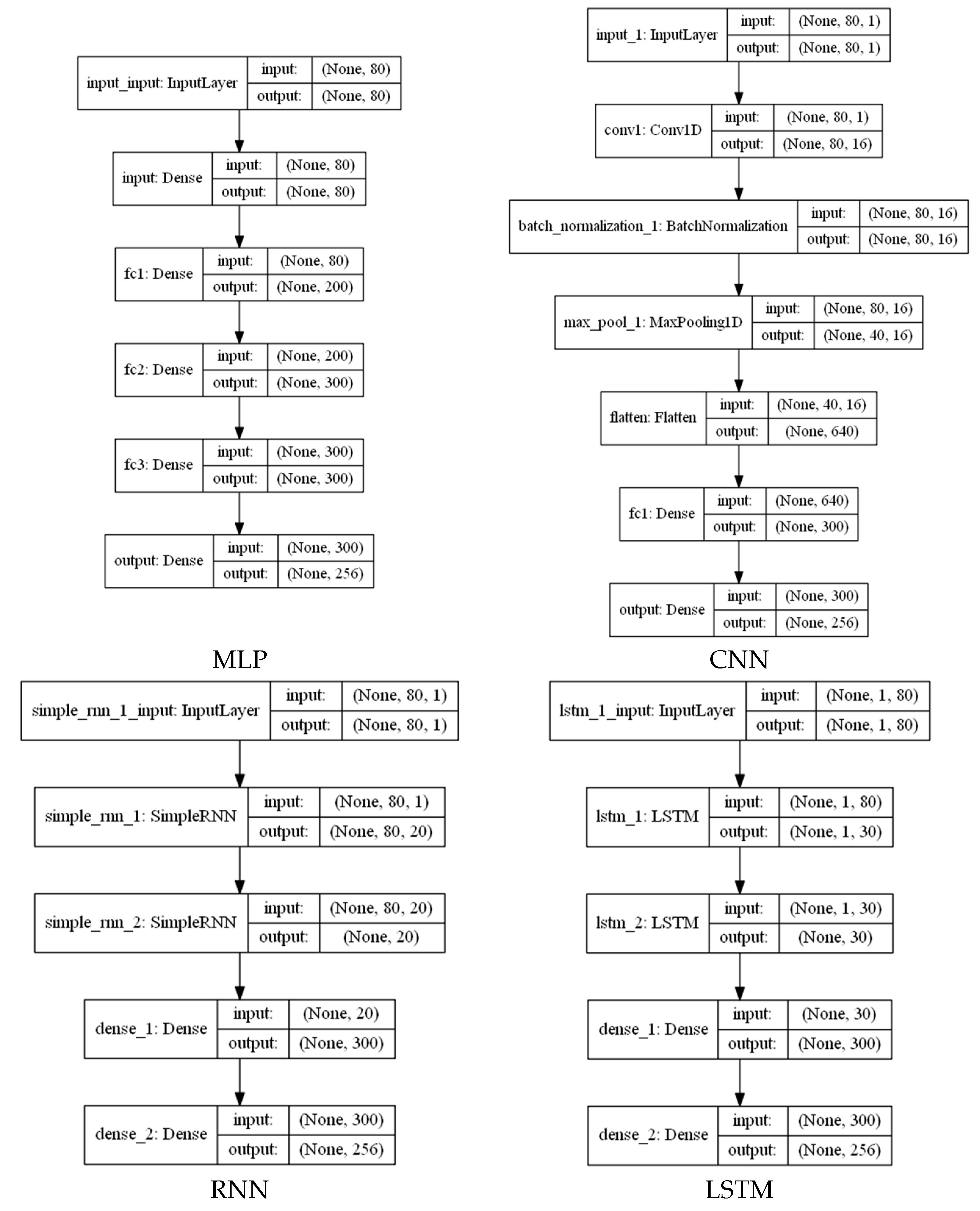
2. Four Deep Learning Models

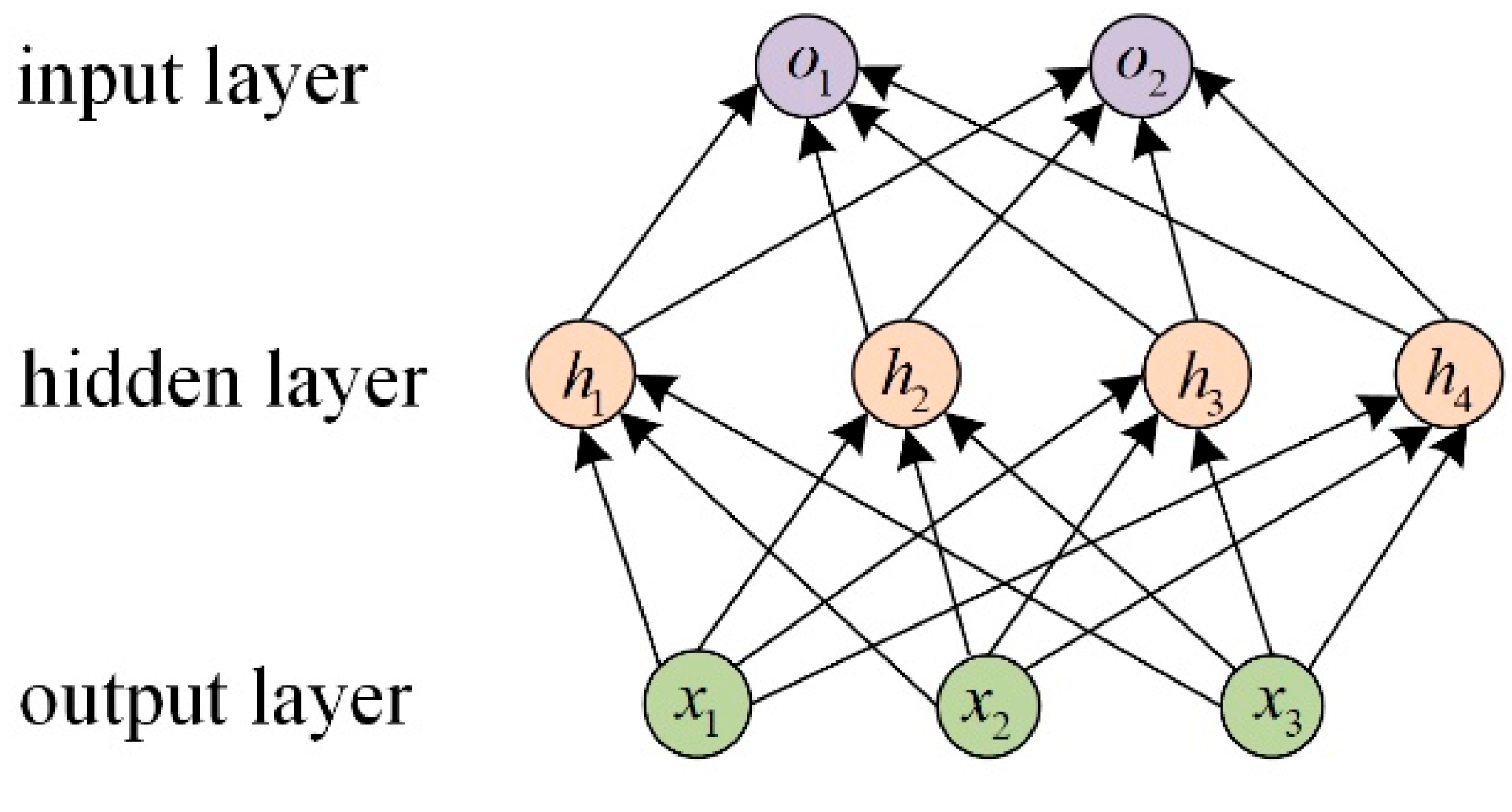
2.1. Multilayer Perceptron

The multilayer perceptron (MLP) is a fully connected neural network composed of multiple perceptron units [24]. Its input and output layers contain at least one hidden layer transformed by the ReLU function or the sigmoid function. It can deal with nonlinear separable problems and has very powerful adaptive and self-learning functions. However, it is difficult to select the number of hidden nodes in the network. Moreover, it is widely used in image recognition, speech recognition, machine translation, and other fields. If s is the operation of the softmax function, λ n is the full connection layer, and σ i is the activation function, then the MLP can be composed of a series of linear functions and nonlinear activation functions, and the function F is expressed as:
F ( x ) = s λ n σ n 1 λ n 1 λ 1 ( x ) = y
Each layer of the MLP is connected to the neurons of adjacent layers, and multiple input data sets are mapped to a single output data set. Let each neuron in the network have a bias value b and an activation function f; the neuron connection weight value between adjacent layers is wi, and i { 1 , , m } ; m is the number of connection layers, and xi represents the input of layer i. Then, the output of each neuron can be expressed as:
o = f ( i = 1 m w i x i + b )
The MLP shown in Figure 1 consists of an input layer, an output layer, and a hidden layer. The number of inputs and outputs is three and two, respectively, and the hidden layer in the middle contains four hidden units.

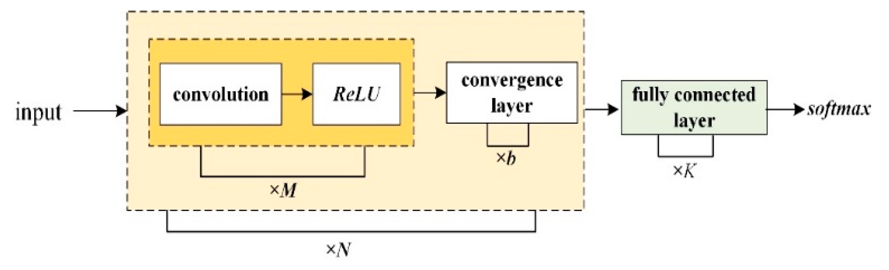
2.2. Convolutional Neural Network

A convolutional neural network (CNN or convnet) is a deep feedforward neural network composed of a convolution layer, a convergence layer, and a full connection layer [25]. It has local connection characteristics and weight sharing and can fit any continuous function. It is a neural network specially used to process data with a similar network structure. CNN-designed neurons have three dimensions: width, height, and depth. However, the scale of parameters will increase sharply with the increase in the number of hidden-layer neurons, which makes the training efficiency of the whole neural network very low and prone to overfitting. Secondly, because the fully connected feedforward network is difficult for extracting the local invariance features of objects, data enhancement methods are needed to improve the performance. The output of the feedforward neural network only depends on the current input, that is, the input is independent, which requires the input and output of data with fixed dimensions. It is difficult to process video, voice, and other timing data. The CNN has a wide range of speech recognition, language detection, document analysis, and image recognition applications. The commonly used structure of the convolution network is shown in Figure 2 below.
A convolutional network stacks N consecutive convolutional blocks and connects K fully connected layers. A convolution block contains consecutive M convolution layers and b pooling layers. Generally, the value range of N is large, and 0 ≤ K ≤ 2, 2 ≤ M ≤ 5; b = 0 or 1:
R e L U ( x ) = m a x ( 0 , 1 ) = 0 , x 0 x , x > 0
The model’s accuracy is obtained by activating the input feature data through the Softmax activation function of the output layer. The number of output values is equal to the number of label categories, which is a single-layer neural network. The loss function corresponding to the activation function is the multiclass Cross-Entropy Loss Function.

2.2.1. Softmax Function

For K scalar x 1 , , x K , the Softmax function can be defined as:
z k = s o f t m a x ( x k ) = exp ( x k ) i = 1 K exp ( x i )
When a K-dimensional vector represents the input of the Softmax function x = x 1 ; ; x K , the Softmax function can be abbreviated as:
z ˜ = s o f t m a x ( x ) = 1 k = 1 K exp ( x k ) exp ( x 1 ) exp ( x K ) = exp ( x ) k = 1 K exp ( x k ) = exp ( x ) 1 K T exp ( x )

2.2.2. Softmax Regression

Softmax regression makes a linear superposition of input features and weights. The Softmax regression model is also called conditional maximum entropy or a logarithmic linear model. If a linear log model is used to model the conditional probability p ( y | x ) , then
p ( y | x ; θ ) = 1 Z ( x ; θ ) exp ( θ T f ( x , y ) ) = 1 y exp ( θ T f y ( x , y ) ) exp ( θ T f ( x , y ) )
The Softmax operation transforms the output into a legal category prediction distribution. For sample i, construct vector y i q so that the y ( i ) element of the discrete value of sample i category is 1 and the rest is 0. The smaller the difference between the predicted probability distribution y ^ ( i ) and the real label probability distribution y ( i ) , the better. However, to make the prediction classification result correct, it only needs to measure the difference between the two probability distributions when calculating the error on the discrete label. We use the Cross-Entropy Loss Function to measure. If the element not 0 or 1 in the vector y ( i ) is set as y j ( i ) , the definition of cross-entropy is as follows:
H ( y ( i ) , y ^ ( i ) ) = j = 1 q y j ( i ) log y ^ j ( i ) = log y ^ y ( i ) ( i )
Assuming that the number of samples in the training data set is n, the Cross-Entropy Loss Function can be defined as:
( Θ ) = 1 n i = 1 n H ( y ( i ) , y ^ ( i ) )
In the above formula, Θ is the model parameter. When each sample has only one label, the corresponding cross-entropy loss is:
( Θ ) = 1 n i = 1 n log y ^ y ( i ) ( i )

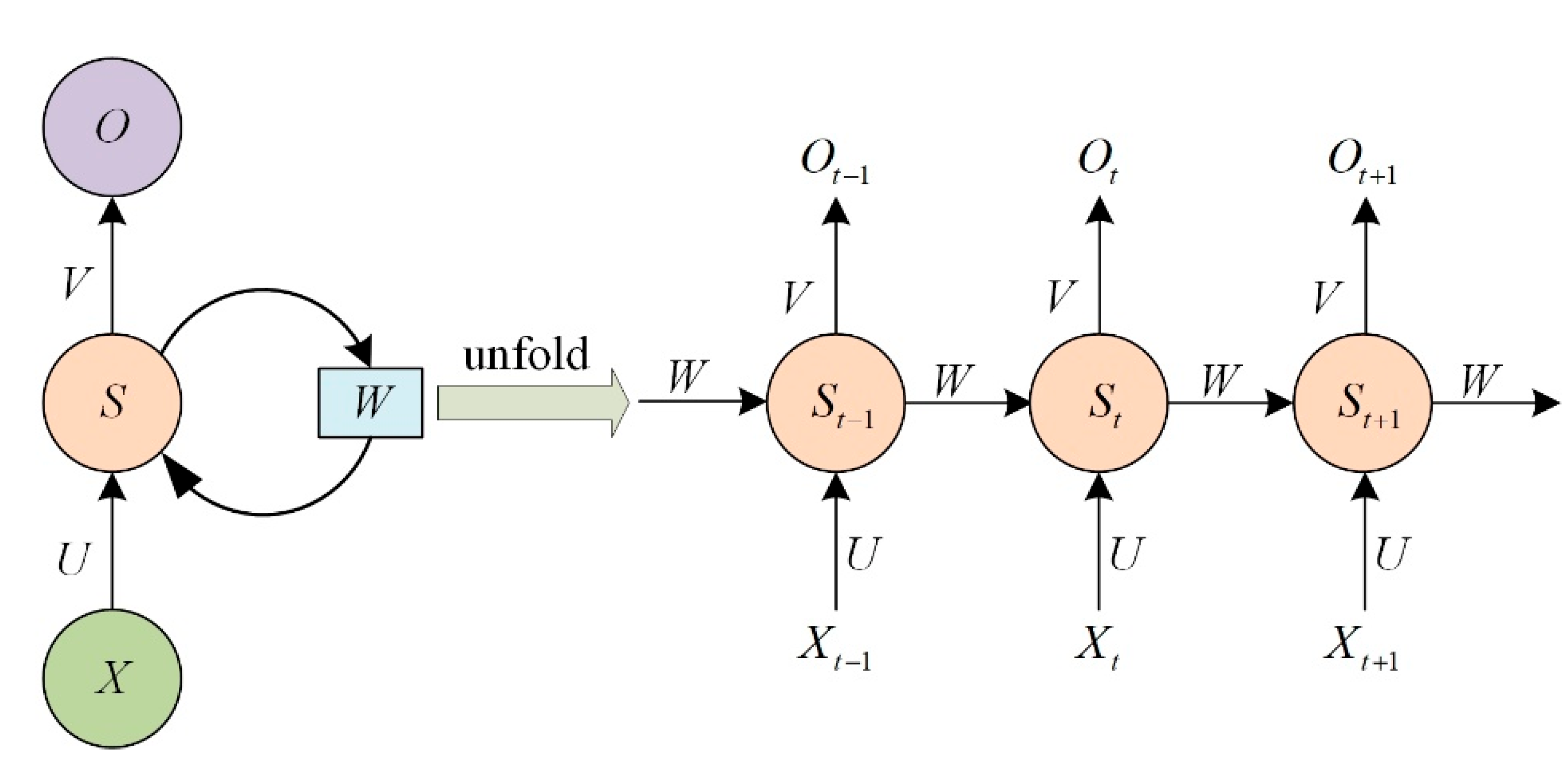
2.3. Recurrent Neural Network

A recurrent neural network (RNN) is a kind of neural network with short-term memory capability that can simulate any program and store the information of previous time steps through a hidden state [26]. Using the neuron with self-feedback, it can process any length of time series data and can be used to mine the time series and semantic information in the data. One time, the back-propagation algorithm is used to learn the parameters, but when the input sequence is too long, the gradient explosion and disappearance problem may occur. Therefore, the gating mechanism is introduced to solve this long-range dependence problem. It can be extended to the recursive neural network (recNN) and the graph neural network (GNN). The RNN is widely used in video processing, speech recognition, text generation, image processing, and other fields. If Xt represents the input of time t, Ot represents the output of time t, and St represents the memory of time t, the cyclic neural network structure diagram is shown in Figure 3 below.
The corresponding expression is:
O t = g ( V S t )
S t = f ( U X t + W S t 1 )

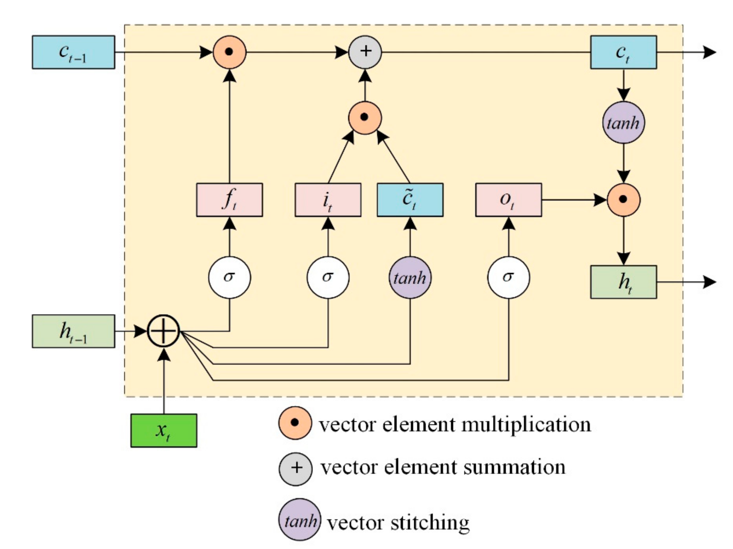
2.4. Long Short-Term Memory Network

To improve the gradient explosion or gradient disappearance problem of the simple recurrent neural network, the Long Short-Term Memory Network (LSTM) based on gating is introduced, which is a variant of a cyclic neural network [27,28] and is widely used in speech recognition, text generation, machine translation, image description, and video marking. Due to its complex structure, it has high computational complexity and is difficult to carry out in-depth learning. To control the path of information transmission, the three gates in the gating mechanism introduced by the LSTM network are the input gate it, the forgetting gate ft, and the output gate ot. The input gate controls the amount of information to be stored in the candidate state c ˜ t at the current time, the output gate determines the amount of information transmitted from the internal state ct at the current time to the external state ht, and the forgetting gate controls whether the internal state ct−1 information at the previous time is retained or discarded. The expression is as follows:
i t = σ ( W i x t + U i h t 1 + b i ) f t = σ ( W f x t + U f h t 1 + b f ) o t = σ ( W o x t + U o h t 1 + b o )
Among them, the input of the current time is xt, σ ( ) is the logistic function, and the corresponding interval of the value range is (0, 1). The recurrent cell structure of the LSTM network is shown in Figure 4 below.
The timing dependency of the LSTM network can be expressed by the following formula:
c ˜ t o t i t f t = t a n h σ σ σ W x t h t 1 + b
c t = f t c t 1 + i t c ˜ t
h t = o t t a n h ( c t )

3. AES-128 Algorithm

On 15 April 1997, the National Institute of Standard Technology (NIST) launched the activity of soliciting AES (Advanced Encryption Standard), which aims to replace the DES (Data Encryption Standard) cryptographic algorithm and determine a new data encryption standard, with a message block length of 128 bits and a key length of 128/192/256 bits or 16/24/32 bytes, faster than triple DES and at least as secure as triple DES. Until 2 October 2000, NIST announced the Rijndael algorithm proposed by Belgian scholars Joan Daemen and Vincent Rijmen as the new AES [29]. The Rijndael block cipher algorithm integrates security, high performance, and adaptability. According to the different key lengths, it is recorded as AES-128, AES-192, and AES-256, respectively. This paper takes the most widely used AES-128 algorithm as the research object and carries out security analysis combined with deep learning and SCA technology.
The state of the AES-128 algorithm corresponds to a 4 × 4 = 16 byte matrix, and the encryption process needs to go through 10 rounds of function iteration operations. Except for the 10th round, every other round needs to go through SubByte, ShiftRow, MixColumn, and AddRoundKey. The tenth round does not include MixColumn. Among them, SubByte is the only nonlinear transformation in the AES algorithm, which constitutes the nonlinear substitution layer of the AES algorithm, that is, the S box. The ShiftRow and MixColumn transformation constitute the linear mixing layer of the AES algorithm, that is, the P box. Therefore, the AES algorithm is a typical SP (substitute-permutation) structure. In this paper, for the 16-bytes data blocks of the AES algorithm state, the “divide and conquer” strategy is adopted to analyze and crack each byte one by one and to finally realize the recovery of all keys. The pseudocode of the AES algorithm is shown in Algorithm 1 below.
Algorithm 1: Preudocode of the AES-128 algorithm
//AES-128 Cipher
//in: 128 bits (plaintext)
//out: 128 bits (ciphertext)
//Nr: number of rounds, Nr = 10
//Nb: number of columns in state, Nb = 4
//w: expanded key K, Nb * (Nr + 1) = 44 words, (1 word = Nb bytes)
state = in;
AddRoundKey (state, w [0, Nb − 1]);
for round = 1 step 1 to Nr − 1 do
 SubBytes (state); // Attack Point, at round 1.
 ShiftRows (state);
 MixColumns (state);
 AddRoundKey (state, w [round * Nb, (round + 1) * Nb − 1]);
end for
SubBytes (state);
ShiftRows (state);
AddRoundKey (state, w [Nr * Nb, (Nr + 1) * Nb − 1]);
out = state;

4. CPA Side-Channel Analysis Based on Deep Learning

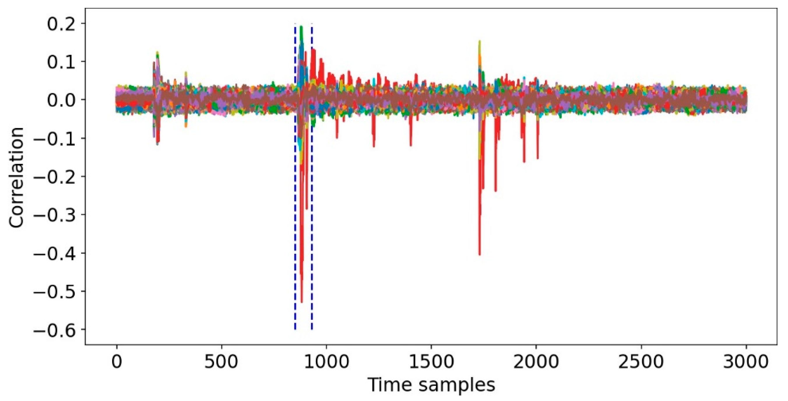
4.1. CPA-Related Principles

The principle of CPA is that the instantaneous energy consumed by electronic equipment during encryption and decryption operations is related to the data written in the register and the operation. Usually, the correlation between the Hamming weight and the voltage of the processed data is studied. The weight of Hamming is introduced as follows:
r ( H , V ) = 1 N i = 1 N ( z H ) i ( z V ) i
In an m-bit microprocessor, binary data are encoded as D = j = 0 m 1 d j 2 j , where bit dj = 0 or 1, and its Hamming weight refers to the number of nonzero symbols in the string, which can be expressed as H ( D ) = j = 0 m 1 d j . In this paper, the Hamming weight model is defined as:
T = a H ( D ) + b + r
In the above formula, a and b are constants, H(D) is the Hamming weight, and r is random noise. The basic idea of CPA is as follows:
(1) The selection of the attack position of the algorithm. The attack point needs to be selected after the key is used. For the AES algorithm, the target attack point is generally selected after the S-box or MixColumn. This paper selects the output position of the first round S-box of the AES-128 cipher algorithm as the target attack point.
(2) Measure of relevance. The Hamming weight and voltage are regarded as two random variables H and V. Through analysis, an expression similar to V i = α H i + β can be obtained to solve the correlation coefficient between them. In this paper, the Pearson correlation coefficient [30] describes the correlation between the Hamming weight and the voltage. The Pearson correlation coefficient is expressed as follows:
r ( H , V ) = 1 N i = 1 N ( z H ) i ( z V ) i
In the above formula z x = x x ¯ σ x , N is the total number of samples selected, and z is the result of the standardization of random variables.
(3) The specific attack process:
Step 1: Randomly select plaintext bytes P 1 , , P N , and input them into the encryption unit of the target cipher algorithm to perform the encryption operation. Then, the power trace in the encryption process, the voltage V is collected, and each power trace contains M sampling points. The power trace refers to the information leaked by different plaintexts in the encryption process under the correct key. In the experiment, the power trace at the same sampling point is selected as the N sample values of the variable V.
Step 2: Generate the corresponding intermediate value by guessing the key and calculating the assumed energy consumption D according to the Hamming weight leakage of the intermediate value.
Step 3: Calculate the correlation coefficient between the assumed energy consumption trace and the measured value. The pseudocode of the attack process is shown in Algorithm 2 below.
Algorithm 2: Randomly select plaintext P 1 , , P N and collect a power trace; each power trace has M sampling points
For byte = 1:16
 For k = 0:255
H = HammingWeight(Sbox(Pbytek)) // Pbyte: The byte-th byte of each Pn
 For m = 1:M
  V = vm // vm: The m-th sampling point of each power trace v
 Corr (k) = r(V,H)
rightkeybyte = find(max{Corr})
When distinguishing whether the key guessed is correct, it is not necessary to find when the attack point is executed, but only to solve the correlation coefficient of all positions and find the maximum value. The point with the greatest correlation corresponds to the correctly guessed key, so the correct key and the output position of the S-box are determined.

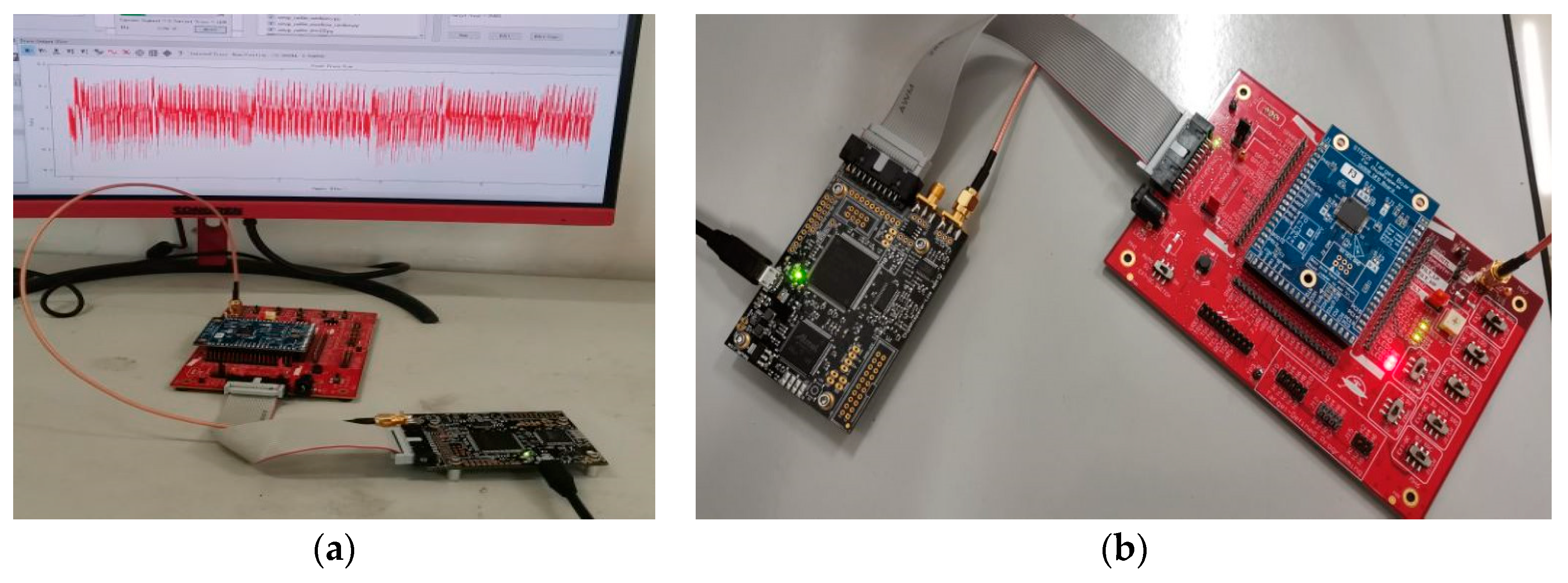
4.2. CPA Experimental Environment Configuration

The computer hardware configuration used in the experiment is Intel® CoreTM i7-7700HQ CPU @ 2.80 GHz and an NVIDIA GeForce GTX 1060 6 GB GPU, combined with the ChipWhisperer physical chip attack platform and the CW308T-STM32F3 demo board running AES-128 cryptographic algorithm, the energy consumption data is sampled at 40 MHz. Combined with the keras2.3.1 [31] and tensorflow2.1.0 [32] deep learning framework, using an open-source package and environment manager python3.6 to compile and execute on the Anaconda Jupiter notebook, after completing the construction, training, and testing of the four models, all experiments are finally completed. The experimental equipment is shown in Figure 5 below.

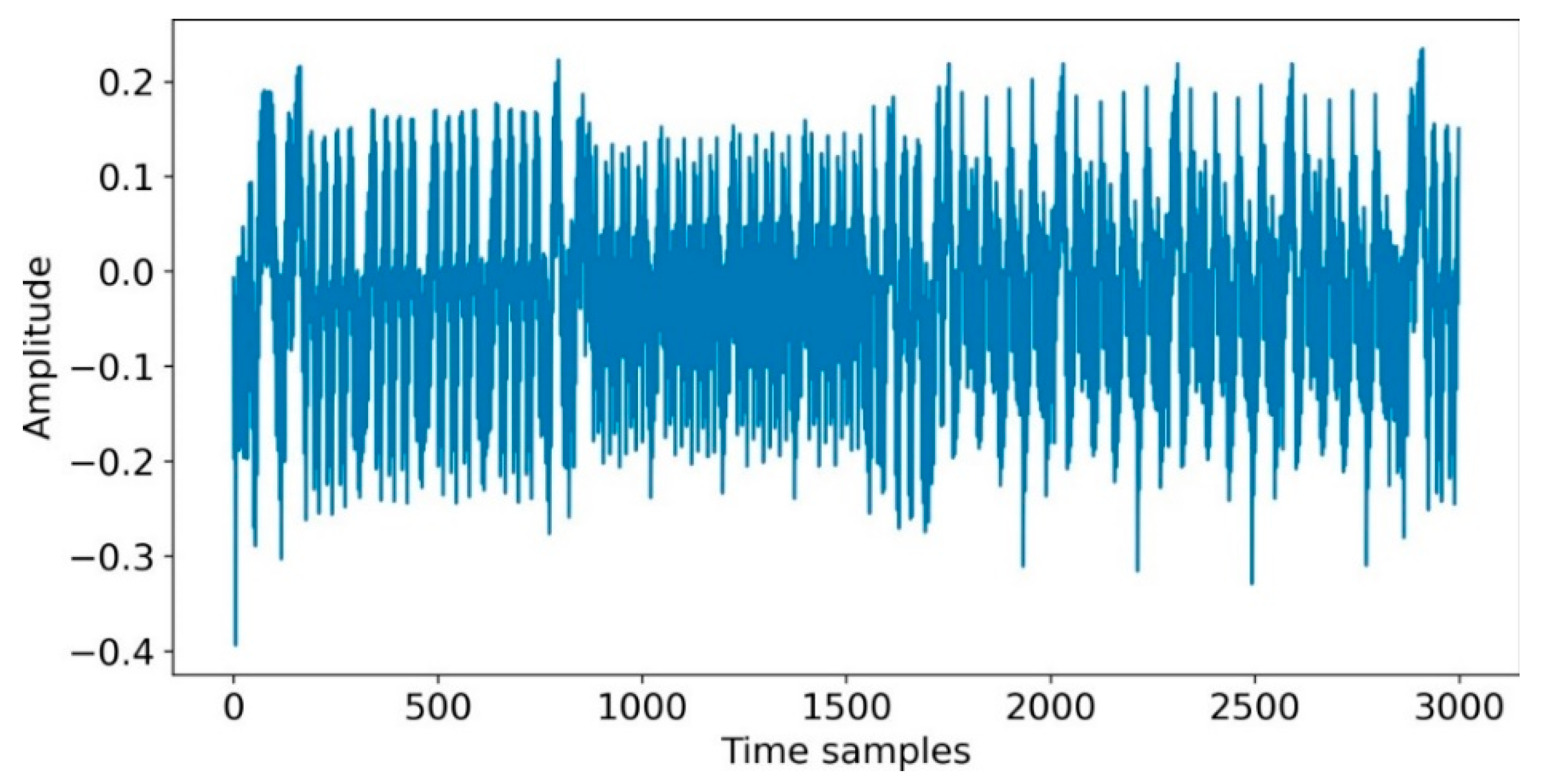
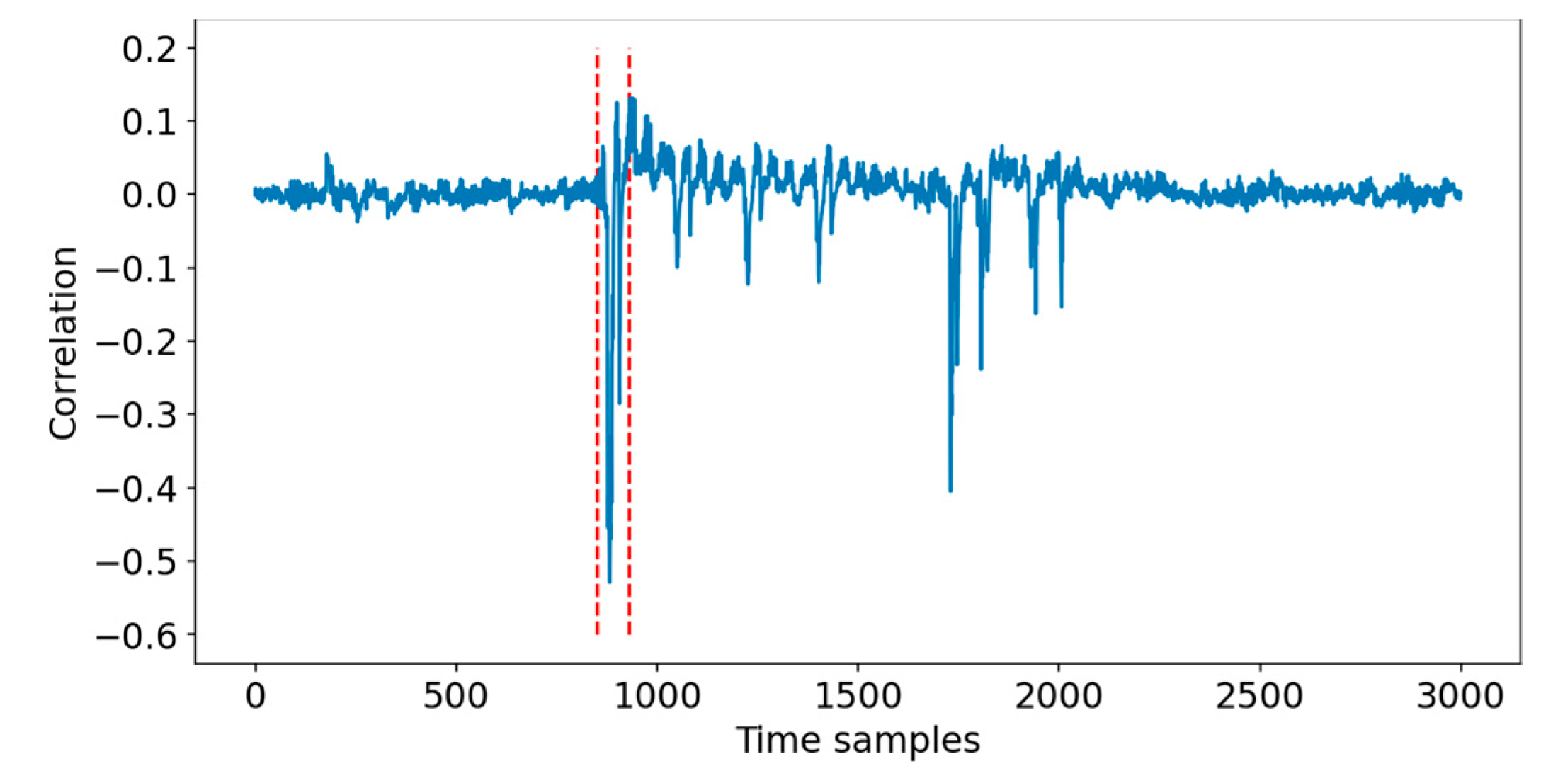
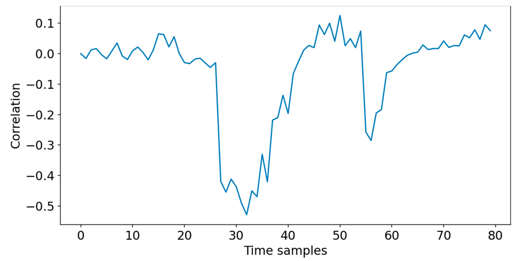
4.3. CPA Experimental Analysis Process

(1) Collection and pre-processing of side-channel data. This experiment uses the ChipWhisperer platform to perform SCA on the AES-128 cryptographic algorithm through the CW308T-STM32F3 demo board. When pre-processing the side channel data, it must first be aligned. Since the ChipWhisperer platform in the experiment has automatically aligned all collected data, this operation can be ignored. When the data are unstable, the variance or the degree of dispersion is large; it is necessary to normalize the data. The sample diagram of the power trace collected in the experiment is shown in Figure 6 below, and each trace contains 3000 data points.
(2) Determine the location of the target attack point. The target attack point in the experiment is the output position of the first round S-box of the AES-128 cryptographic algorithm, and its output state can be expressed as s t a t e 0 = S b o x ( p 0 k 0 ) , where subscript 0 represents the attack on the first byte of the key stream, S-box represents the byte substitution operation in the S-box, and p and k represent the input random plaintext and random key information, respectively. Thus, the first byte K[0] of the key of the first round is recovered.
(3) CPA attack on the power trace to find the data interest interval. The point of interest is the interval range of the encryption operation corresponding to the location of the attack point in a complete power trace, that is, the interesting interval. The detailed steps of CPA are as follows:
Firstly, the power trace matrix T of the original side-channel data is established. A total of 50,000 energy consumption tracks were collected in this experiment, with 3000 sampling points on each track. Therefore, the energy consumption trajectory matrix T can be established, and its dimension is 50,000 × 3000.
Secondly, construct the output state matrix S. For an 8-bit key byte, the value of the key space ranges from 0 to 255, with a total of 256 possibilities. For all possible key values, obtain the output state matrix S of all target positions, and the matrix dimension is 50,000 × 256.
Finally, using the Pearson correlation coefficient [30] calculation method, the correlation between the power trace matrix T and the output state matrix S is calculated, and the final correlation coefficient matrix R is obtained with a dimension of 3000 × 256, which represents the correlation coefficients of all possible key operations at all timing sampling points. Thus, the data point’s position with the greatest correlation with the key in the power race is determined. The value range of the final interest interval is [850:930], with a total of 80 sampling points. Figure 7 shows the waveform of power trace information related to the first round of the encryption operation in the CPA of a single power trace. Figure 8 is the amplification result of the corresponding interest interval in the CPA, that is, it contains the energy consumption information of the first round of the S-box byte substitution operation.
(4) According to the position of the determined interest interval, the original side-channel data are subjected to dimensionality reduction processing. In this experiment, the range of interest intervals is 850~930, that is, the original 3000-time series sampling points are reduced to 80, which greatly reduces the computational complexity of the deep learning model and improves the computational efficiency. For the power consumption data of the CW308T-STM32F3 demo board, the correlation curve of all possible keys analyzed by CPA technology is shown in Figure 9 below. The range within the dotted line in the figure is the corresponding interval of the target byte in the experiment.
(5) After processing all side-channel data, the entire dataset is divided into training and test sets. The detailed results of this experiment can be found in Section 5.
(6) Building deep learning models. Under the Keras framework, the four deep learning models of MLP, CNN, RNN, and LSTM are built, and the model structure, parameter scale, and hyperparameters of each model under different scale data are the same. Model example diagrams are shown in Figure 10 below. The RNN model has the smallest parameter scale, with only 84,616 parameters, and the CNN model has the largest parameter scale, with 269,484 parameters. In addition, the parameters of MLP and LSTM are 250,336 and 106,996, respectively.
The hyperparameter settings corresponding to each model in all experiments in this paper are shown in Table 1 below.
(7) Train and test each model. All models are trained and tested using datasets of different sizes. The model accuracy is obtained by activating the input feature data through the Softmax activation function of the last layer, that is, the output layer, which is used to characterize and evaluate the classification ability of the model. To describe the degree of deviation between the predicted value of each model and the actual value, that is, to test the robustness of each model, the multicategory cross-entropy loss function is used in this experiment to calculate the loss value of the model. The Adam optimizer [33] is used for each model.
(8) Recover key byte information. This experiment uses the rank function to calculate the key recovery ability of each deep learning model. Using the training model to predict the test set and get a score vector D, each test data corresponds to a vector D. Then, multiply the D results of multiple data, and sort the data in the matrix according to the multiplied results (in descending order) until the position of the correct key is ranked at the highest position. The corresponding position number is 0, and the rank can be calculated to be 0. The number N of test data used in this process indicates the minimum number of power traces for the model to successfully recover the correct key.

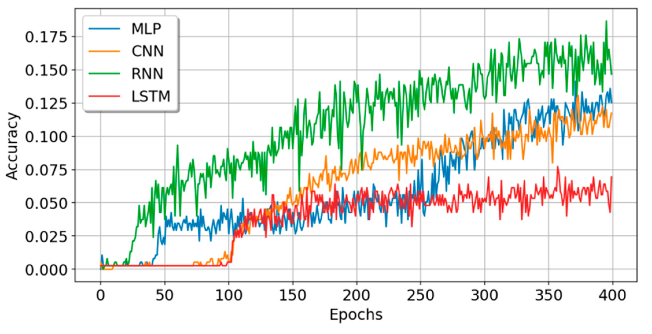
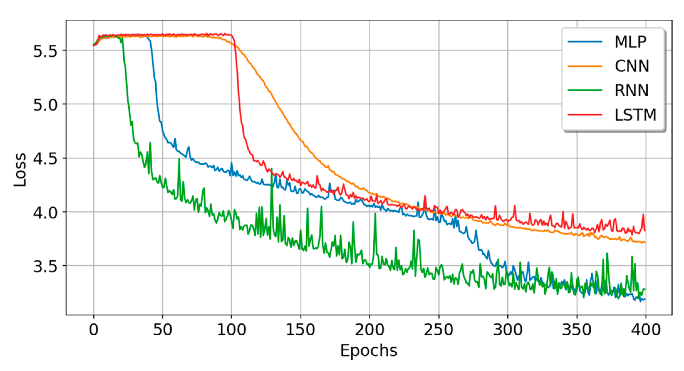
5. Experiment and Model Evaluation

5.1. Experiment A: Small Sample Data Experiment

Under the small data set sample, the experiment uses 1500 random key data sets and randomly divides 1200 training sets and 300 test sets, accounting for 4:1, respectively. The training set is used for model learning and training, and the testing set is used to characterize the generalization ability of the model. To describe the experimental results more accurately, the results recorded in all experiments in this paper are the average results with epochs between 350 and 400. Four deep learning models are used to conduct side-channel analysis experiments on the demo board. The final experimental results of each model classification are shown in Figure 11, Figure 12, Figure 13 and Figure 14, which represent the training accuracy, training loss value, training time, and training rank value of each model when the epochs are 400 and are analyzed in detail.
From the experimental performance of each model on the demo board, it can be seen that in the training of the first 50 epochs, with the increase in the number of iterations, the RNN and MLP models converge rapidly. The accuracy rose to 0.0373 and 0.0187, respectively, and the loss dropped to 4.2227 and 4.7532, respectively. During this period, the training accuracy and loss value curves of the CNN and LSTM models hardly fluctuated. At the 50th epoch, the accuracy of both on the training set was 0.0027, and the loss values were 5.6303 and 5.6518, respectively. After the 100th epoch, the training accuracy and loss values of the CNN and LSTM models did not change significantly. For example, at the 150th epoch, the training accuracies of the RNN, CNN, MLP, and LSTM models reached 0.0907, 0.0480, 0.0427, and 0.0347, respectively, and the model loss values were 3.8305, 4.6636, 4.2096, and 4.2431, respectively. With the increase in the number of iterations, the training accuracy and loss value curves of each model gradually converge smoothly and become stable. When the training reaches the 400th epoch, each model achieves the optimal effect. Between the 350th and 400th epochs, the average training accuracies of the RNN, CNN, MLP, and LSTM are 0.2471, 0.1438, 0.1399, and 0.0676, respectively, the training loss values are 2.5843, 3.4043, 3.0573, and 3.6028, the test accuracies are 0.1300, 0.0940, 0.1180, 0.0600, and the test loss values are 3.4500, 3.6542, 3.1467, and 3.8582, respectively. There is no overfitting phenomenon in each model. On the whole, the RNN model has the highest training accuracy and the smallest loss value, but the volatility is too large. The accuracy of the MLP model is comparable to the CNN model, but the MLP model has a slower convergence speed and the CNN model is more stable. The LSTM model has the least volatility and is smooth and stable, but the accuracy is too low.
Figure 13 shows the training time of each model when the epoch is 400. The training time of MLP is the shortest, which is the same as that of the CNN model, saving 34% and 81% compared to the RNN and LSTM models, respectively. It can be seen from Figure 14 that with the increase in the number of power traces, the rank value of each model gradually decreases to be flat, and the RNN model has the most obvious change. The rank values of the final MLP, CNN, RNN, and LSTM models are 3, 2, 3, and 4, respectively. The CNN model has the smallest rank value, and only two traces are needed to recover the correct key bytes.
The specific parameters and experimental results of each model in Experiment A are shown in Table 2 below.

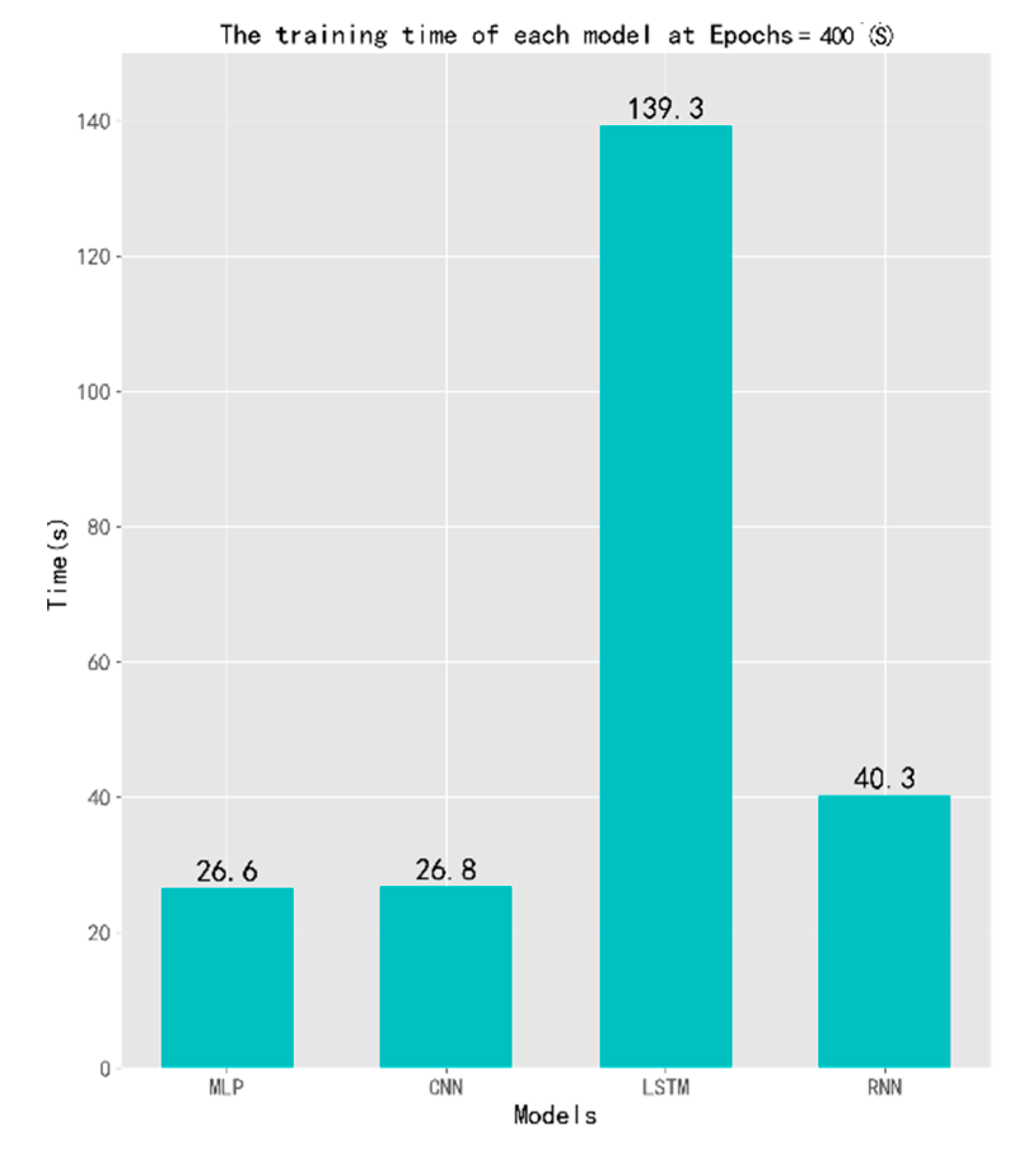
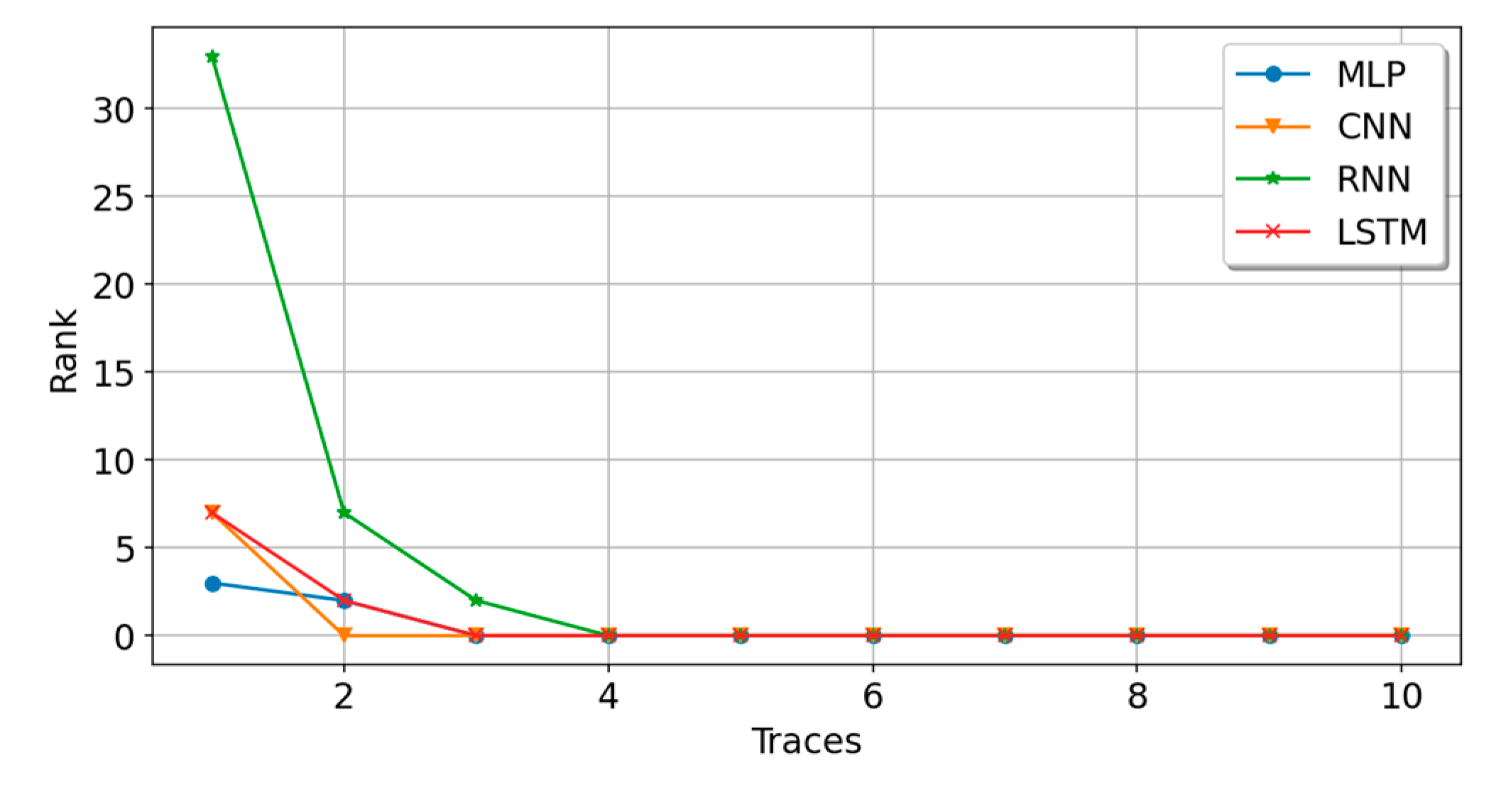
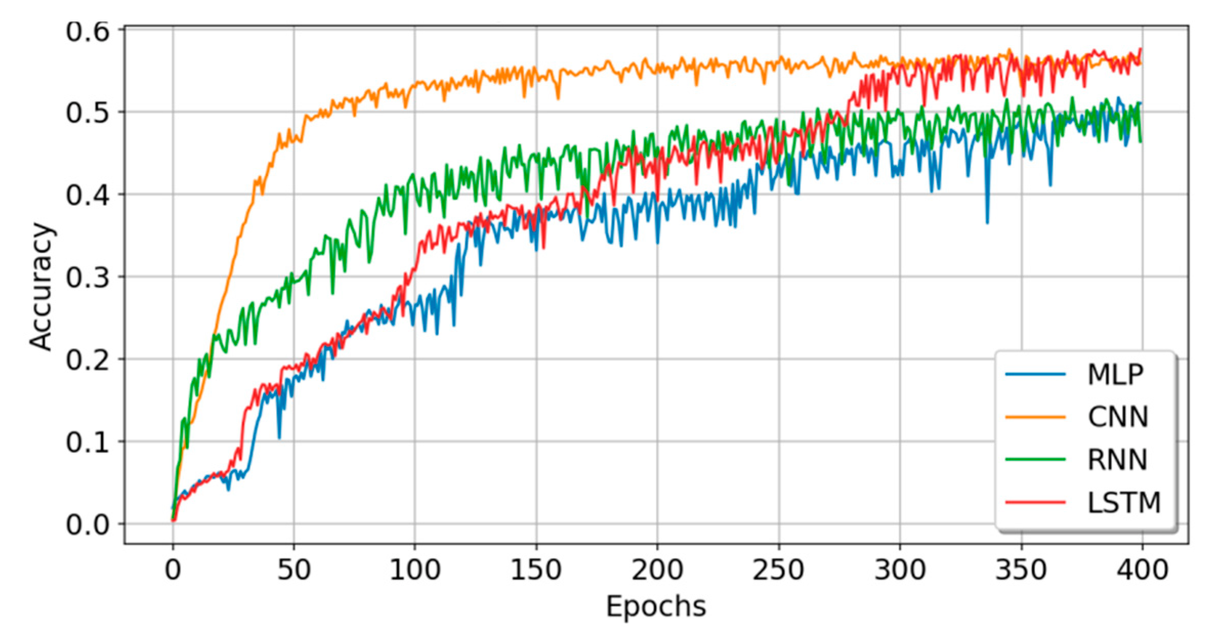
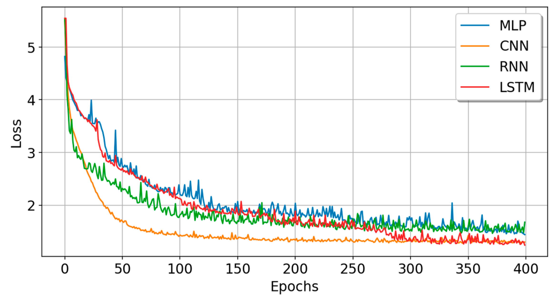
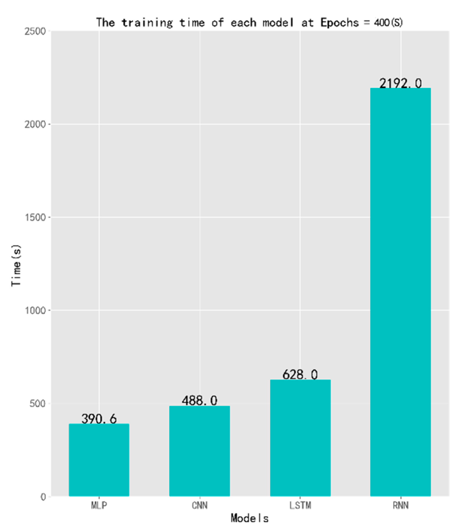
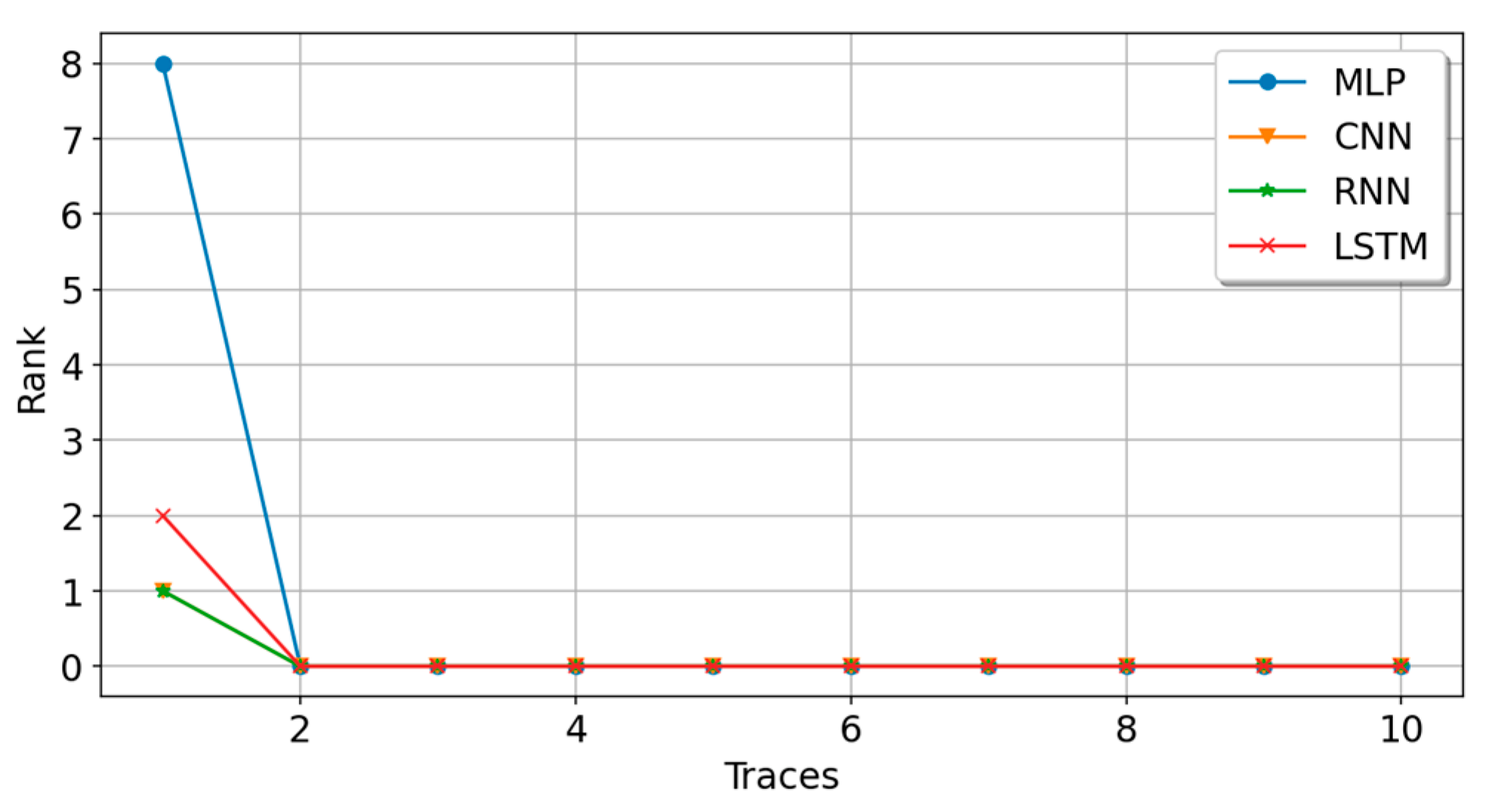
5.2. Experiment B: Sufficient Sample Data Experiment

With sufficient data set samples, the experiment uses 50,000 random key data sets and randomly divides 45,000 training sets and 5000 test sets, accounting for 9:1, respectively. Four deep learning models are used to conduct side-channel analysis experiments on the encrypted board. The final experimental results of each model classification are shown in Figure 15, Figure 16, Figure 17 and Figure 18, which represent the training accuracy, training loss value, training time, and training rank value of each model when the epoch is 400 and analyzed in detail.
It can be seen from the experimental performance of each model on the demo board that in the training of the first 50 epochs, with the increase in the number of iterations, the four models of CNN, RNN, LSTM, and MLP converge rapidly. At the 50th epoch, the accuracy of the model on the training set rose to 0.4637, 0.2922, 0.1879, and 0.1772, and the loss dropped to 0.5292, 0.4116, 0.3071, and 0.2656, respectively. After the 50th epoch, the CNN model converged at a slow speed. After the 300th epoch, with the increase in the number of iterations, the training accuracy and loss value curves of each model gradually converged smoothly and tended to be stable. At 400 epochs, each model achieves the optimal effect. Between the 350th and 400th epochs, the average training accuracies of the CNN, LSTM, RNN, and MLP are 0.5745, 0.5666, 0.5128, and 0.4944, respectively, the training loss values are 1.2589, 1.2700, 1.4618, and 1.4880, the test accuracies are 0.5496, 0.5680, 0.4550, 0.5084, and the test loss values are 1.3214, 1.2813, 1.6926, and 1.4599, respectively. The MLP and LSTM models show a slight overfitting phenomenon. Overall, the CNN model has the highest training accuracy and the smallest loss value, and the model has the strongest model stability. The accuracy of the RNN and MLP models ranks second, and the convergence speed is also faster, but the training loss value is higher. Although the training loss value of the LSTM is low, the convergence speed is slow and the stability is not very good.
Figure 17 shows the training time of each model when the epoch is 400. The MLP has the shortest training time, saving 20%, 38%, and 82%, respectively, compared with the CNN, LSTM, and RNN models. As can be seen from Figure 18, with the increase in the number of power traces, the rank value of each model gradually decreases to a flat level, among which the change of the MLP model is the most obvious. Finally, the rank values of the MLP, CNN, RNN, and LSTM are all 2.
The specific parameters and experimental results of each model in Experiment B are shown in Table 3 below.

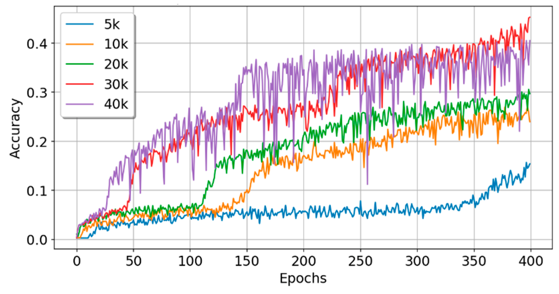
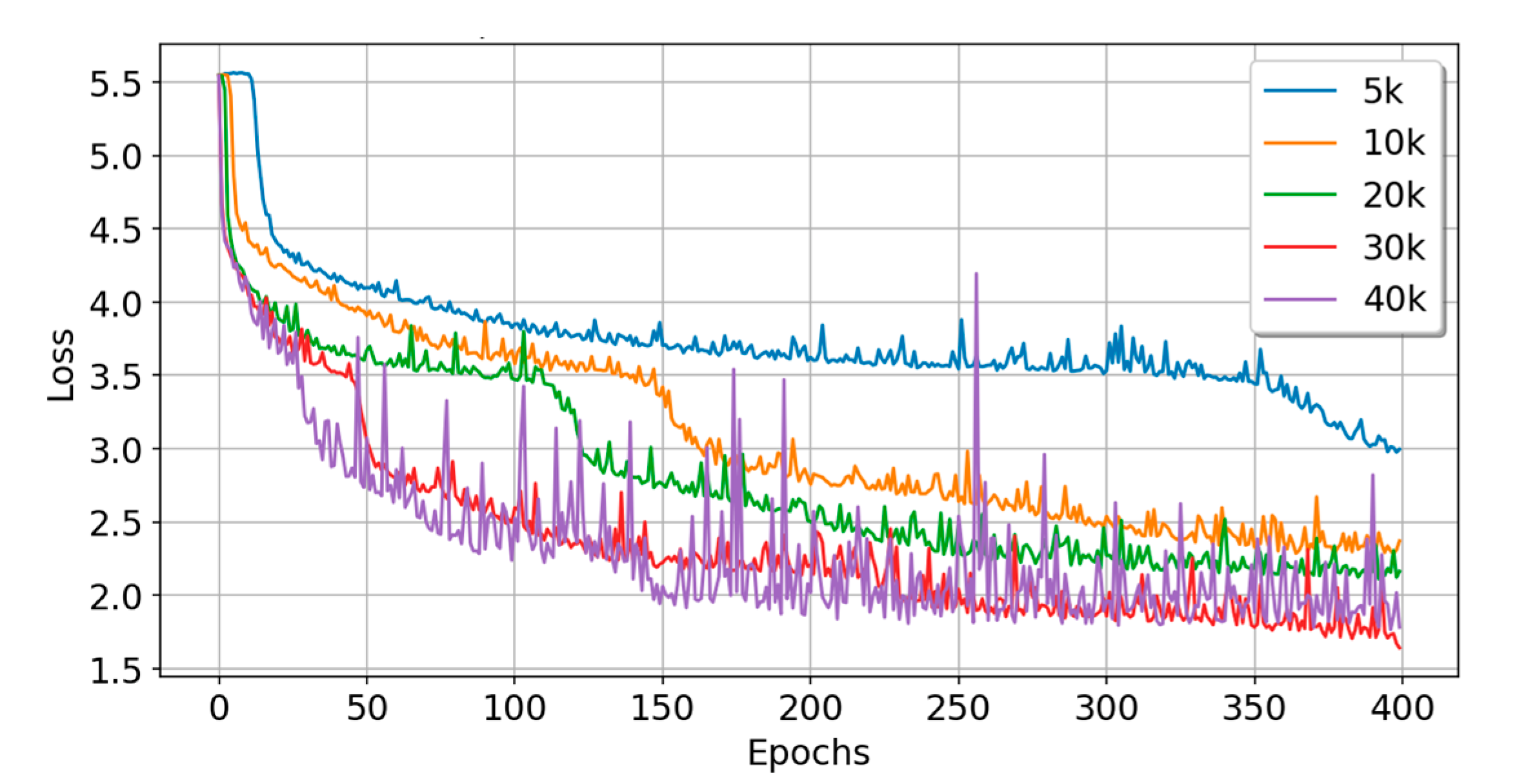
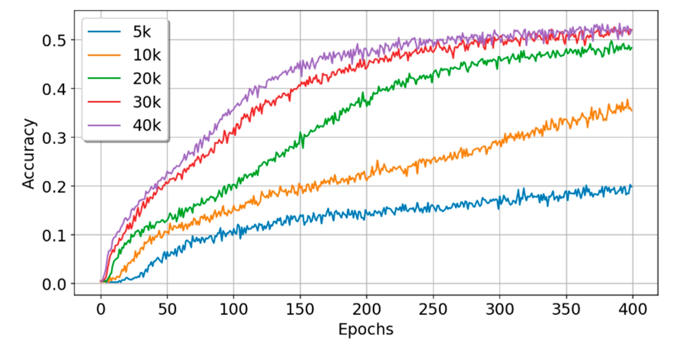
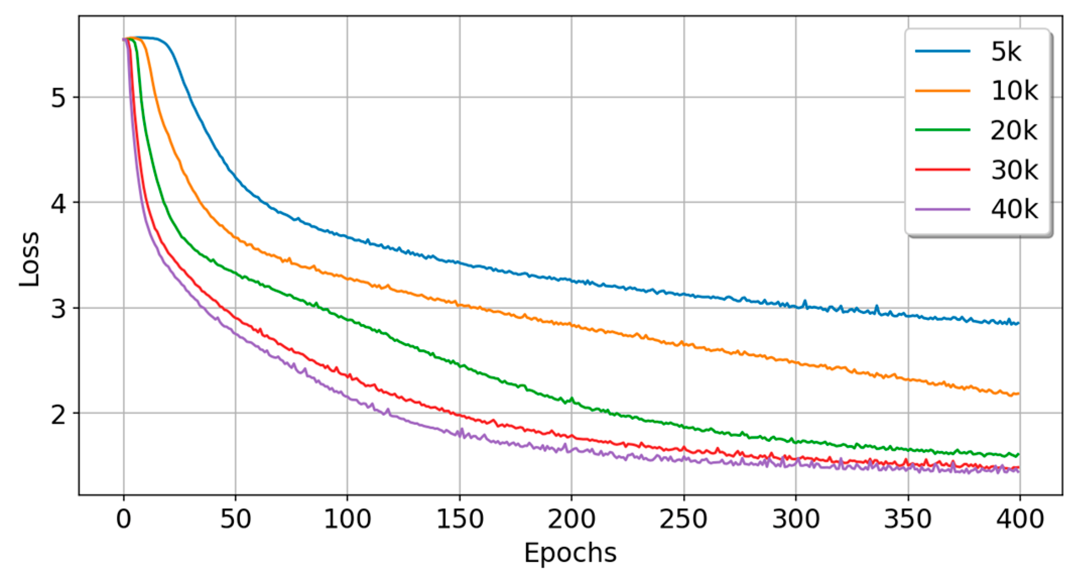
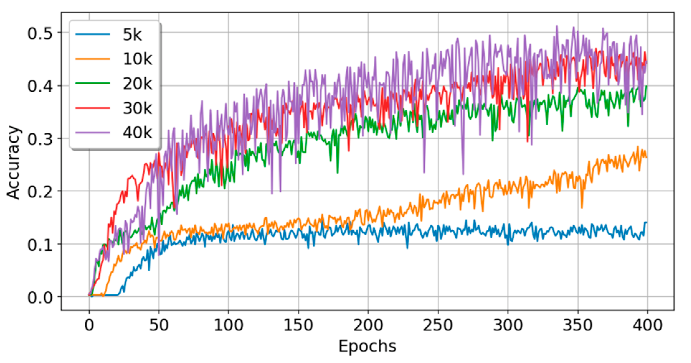
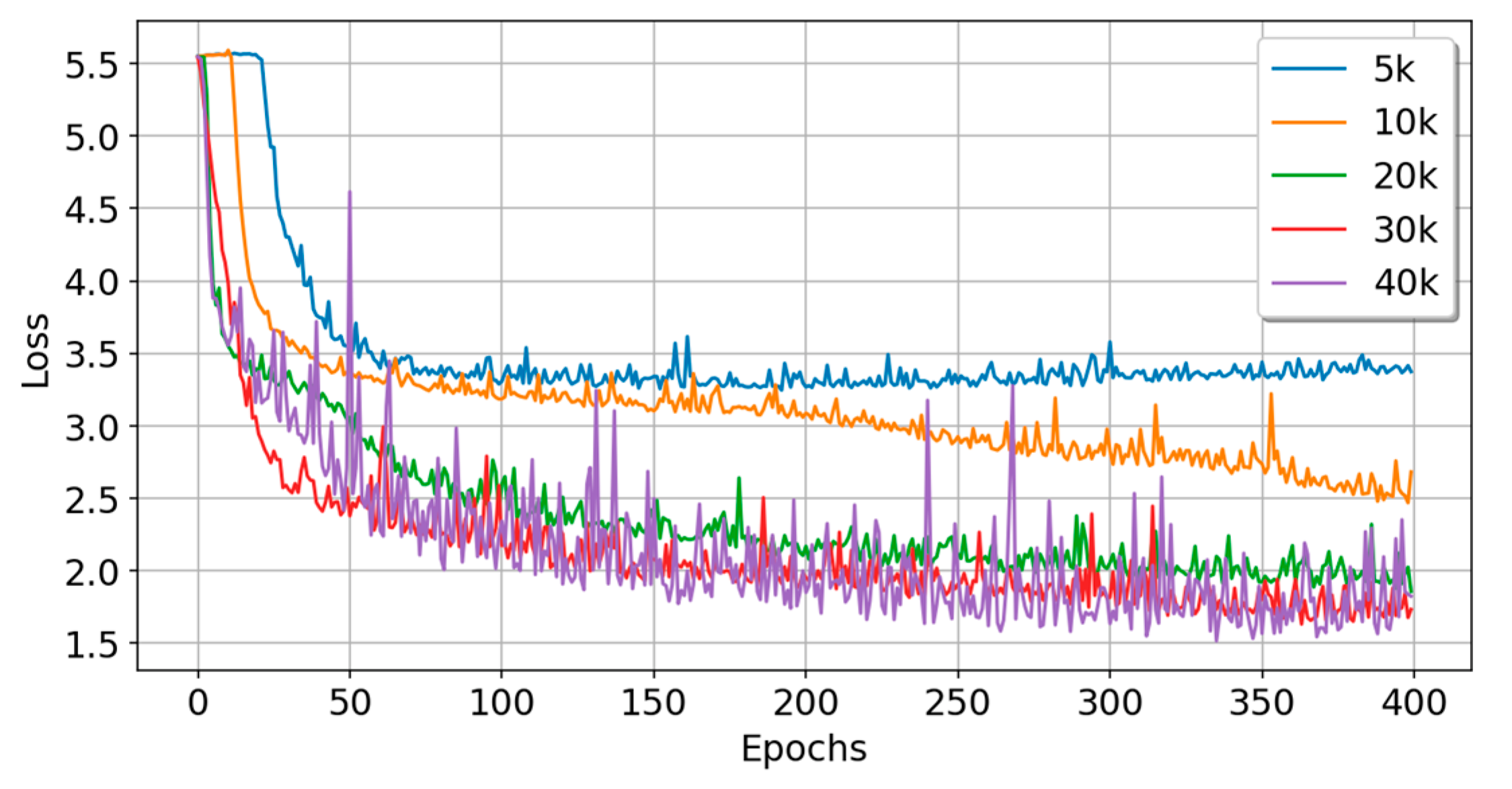
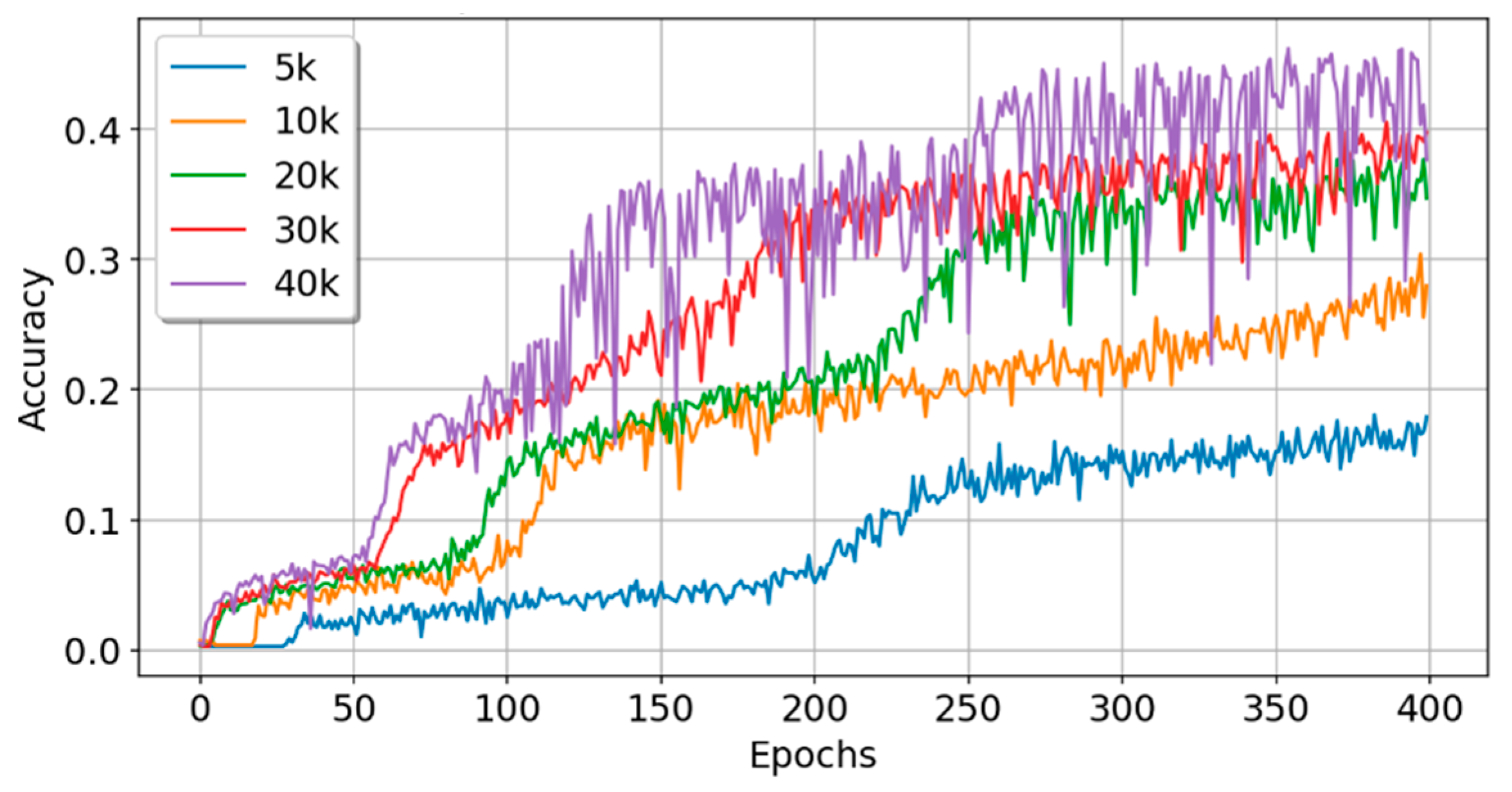
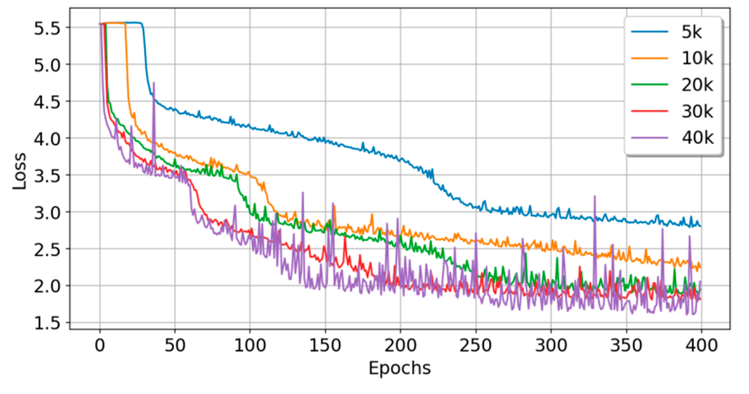
5.3. Experiment C: Experiments with Sample Data of Different Scales

In Experiment C, five data sets of different sizes were used, and each data set was randomly divided into training and test sets on a 9:1 scale. Four in-depth learning models are used to perform side-channel analysis experiments on the demo board. The final experimental results of each model classification are as follows and analyzed in detail. Figure 19 and Figure 20 show the performance of MLP for different size data and MLP loss values under different scales of data, respectively.
For the MLP model, in the training of the first 50 epochs, with the increase in the number of iterations, the model converges rapidly under the number of 40k and 30k data. At the 100th epoch, the accuracy of the model under the amount of 40k, 30k, 20k, and 10k data increases to 0.2028, 0.2082, 0.0626, and 0.0585 respectively, and the loss value decreases to 2.5285, 2.5969, 3.4728 and 3.5789, respectively. After the 100th epoch, the training accuracy of the MLP model changes significantly under each scale data. With the increase in iteration time, the training accuracy and loss value curve of the MLP model under different scale data gradually converge smoothly and tend to be stable. Between 350 and 400 epochs, the average training accuracy of the MLP under 5k, 10k, 20k, 30k, and 40k data volume are 0.1358, 0.2606, 0.2884, 0.4164, and 0.4023, respectively, the training loss values are 3.0848, 2.2648, 2.1439, 1.7370, and 1.7705, respectively, the test accuracy rates are 0.1480, 0.2470, 0.3055, 0.4350, and 0.4145, respectively, and the test loss values are 2.9956, 2.3530, 2.1393, 1.6421, and 1.7597, respectively. There is no fitting phenomenon in MLP under 10k data volume. The rank value under this data volume is 3, and the rank value under other data volumes is 2. For the MLP model, in the training of the first 50 epochs, with the increase in the number of iterations, the model converges quickly under the data volume of 40k and 30k, and at the 100th epochs, the model is under the data volume of 40k, 30k, 20k, and 10k. The accuracies rose to 0.2028, 0.2082, 0.0626, and 0.0585, respectively, and the loss values dropped to 2.5285, 2.5969, 3.4728, and 3.5789, respectively. After the 100th epoch, the training accuracy of the MLP model under various scales of data has changed significantly. With the increase in the number of iterations, the training accuracy and loss curve of the MLP model under different scales of data gradually converge smoothly and tend to be stable. Between the 350th and 400th epochs, the average training accuracy of the MLP under 5k, 10k, 20k, 30k, and 40k data volumes is 0.1358, 0.2606, 0.2884, 0.4164, 0.4023, the training loss values are 3.0848, 2.2648, 2.1439, 1.7370, 1.7705, the test accuracy rates are 0.1480, 0.2470, 0.3055, 0.4350, 0.4145, respectively, the test loss values are 2.9956, 2.3530, 2.1393, 1.6421, 1.7597, and there is no overfitting phenomenon in MLP only under 10k data volume. The rank value of the data volume is 3, and the rank value of the rest of the data volume is 2.
The specific parameters and experimental results of the MLP model are shown in Table 4 below.
Figure 21 and Figure 22 show the performance of CNN for different size data and CNN loss values under different scales of data, respectively. For the CNN model, during the training of the first 100 epochs, the model fluctuated significantly with the increase in the number of iterations. At the 100th epoch, the accuracy of the model under 40k, 30k, 20k, 10k, and 5k data increased to 0.3197, 0.3197, 0.2033, 0.1599, and 0.1125, respectively, and the loss value decreased to 2.3388, 2.3388, 2.8812, 3.2683, and 3.6635, respectively. With the increase in the number of iterations, after the 300th epoch, the training accuracy and loss value curve of the MLP model under different scale data gradually converge smoothly and tend to be stable. Between 350 and 400 epochs, the average training accuracy of the MLP under 5k, 10k, 20k, 30k, and 40k data volume is 0.3045, 0.3826, 0.5258, 0.5352, and 0.5441, respectively, the training loss values are 2.4804, 2.1234, 1.4856, 1.4234, and 1.3806, respectively, and the test accuracy rates are 0.2180, 0.3450, 0.4820, 0.5133, and 0.5265, respectively. The test loss values are 2.8696, 2.2371, 1.6300, 1.4520, and 1.4232, respectively. There is no fitting phenomenon of MLP under each data volume, and the rank value is 2.
The specific parameters and experimental results of the CNN model are shown in Table 5 below.
Figure 23 and Figure 24 show the performance of RNN for different size data and RNN loss values under different scales of data, respectively. For the RNN model, during the training of the first 100 epochs, the model converges rapidly with the increase in the number of iterations. At the 100th epoch, the accuracy of the model under the data of 40k, 30k, 20k, 10k, and 5k increases to 0.3067, 0.3229, 0.2267, 0.1393, and 0.1245, respectively, and the loss value decreases to 2.3427, 2.1726, 2.5977, 3.1857, and 3.3066, respectively. With the increase in iteration time, the training accuracy and loss value curve of the MLP model under different scale data gradually converge smoothly and tend to be stable. Between 350 and 400 epochs, the average training accuracy of the MLP under 5k, 10k, 20k, 30k, and 40k data volume is 0.2025, 02809, 0.4281, 0.4818, and 0.5237, respectively, the training loss values are 2.7272, 2.3556, 1.7523, 1.5794, and 1.4271, respectively, and the test accuracy rates are 0.1100, 0.2350, 0.4105, 0.4390, and 0.4265, respectively. The test loss values are 3.5471, 2.7587, 1.8600, 1.7173, and 1.8233, respectively. There is no fitting phenomenon of RNN under each data volume. The rank value under 5k data volume is 3, and the rank value under other data volumes is 2.
The specific parameters and experimental results of the RNN model are shown in Table 6 below.
Figure 25 and Figure 26 show the performance of LSTM for different size data and LSTM loss values under different scales of data, respectively. For the LSTM model, during the training of the first 100 epochs, with the number of iterations, the model has no obvious fluctuation under the amount of 5k data. At the 100th epoch, the accuracy of the model under the number of 40k, 30k, 20k, 10k, and 5k data increased to 0.1922, 0.1825, 0.1448, 0.0837, and 0.0252, respectively, and the loss value decreased to 2.6289, 2.6858, 2.9755, 3.4882, and 4.1442, respectively. With the increase in iteration time, the training accuracy and loss value curve of the MLP model under different scale data gradually converge smoothly and tend to be stable. Between 350 and 400 epochs, the average training accuracy of MLP under 5k, 10k, 20k, 30k, and 40k data volume is 0.1932, 0.2820, 0.3826, 0.3954, and 0.4671, respectively, the training loss values are 2.6546, 2.2234, 1.8559, 1.7949, and 1.5768, respectively, and the test accuracy rates are 0.1780, 0.2770, 0.3695, 0.3863, and 0.3718, respectively. The test loss values are 2.8335, 2.2410, 1.9201, 1.8032, and 2.0258, respectively. There is no fitting phenomenon of the LSTM under each data volume. The rank value under 5k and 20k data volumes are 3, and the rank value under other data volumes is 2.
The specific parameters and experimental results of the LSTM model are shown in Table 7 below.
Overall, the model accuracy does not necessarily have a linear relationship with the amount of training data. Except for the MLP model, the other three models have no overfitting phenomenon. In terms of training time and accuracy, under different sample data, the CNN model has the highest training accuracy, small training loss value, the shortest time consumption, and the lowest model construction cost, but its parameter scale is the largest, and its structure is complex. The RNN model has the smallest parameter scale and relatively high model accuracy, but the training takes the longest time and requires a lot of time and resources. With the increase in sample data, the accuracy of the LSTM model increases the fastest, which is more suitable for data processing in the case of large-scale samples. However, at this time, the stability of the model is slightly poor, the volatility is large, and the convergence speed is slow.

6. Conclusions

Since deep learning can learn data directly from raw power trajectories, there is no need to rely on artificially designed features or assumptions. Further, the side-channel analysis based on deep learning can directly predict the target intermediate value through the training data set, further simplifying the attack design and reducing the requirements for professional knowledge in specific fields. Based on the above two points, deep learning technology can study the SCA.
By combining the ChipWhisperer experimental platform with the CW308T-STM demo board, this paper extracts the power trace in the encryption process of the unmasked AES-128 cryptographic algorithm and takes it as the experimental data set. Using the established MLP, CNN, RNN, and LSTM models, this paper trains and tests from small data set samples to sufficient data sets and data samples of different scales, and the quantitative experiments of each deep learning model in SCA are deeply studied to evaluate the effectiveness of each deep learning model for subsequent improvement. The experimental results show that the CNN model has better comprehensive performance among all models under the existing data set. From the visualization results of model accuracy and loss, it can be fully demonstrated that the accuracy of its classifier is very high, the loss is very low, and the stability of the model is better. During the whole training process, the experimental curve of the CNN model is smooth, and there is no violent jitter, which means it has stronger robustness. The training time is also short, and the rank value of the side-channel attack is very low. Only two tracks are needed to recover the correct key byte information.
However, compared to the ChipWhisperer experimental platform, the actual test environment has low signal-to-noise ratio data sets or other more complex interference situations. Therefore, to improve the security protection capability of cryptographic equipment, it is necessary to further study the data sets with less obvious information characteristics, and to thus analyze and evaluate the comprehensive performance of each deep learning model in SCA. At the same time, given the complexity of the attack process and implementation details in the SCA experiment, the research direction of the future should investigate the possibility of using statistical testing, computing information entropy, and other formal methods to automatically analyze and evaluate the strength of the encryption system against a side-channel attack.

Author Contributions

Conceptualization, L.C. and Y.W.; methodology, L.C.; validation, L.C. and Y.W.; formal analysis, L.C. and S.H.; investigation, X.P.; resources, Y.W.; data curation, X.P.; writing—original draft preparation, L.C. and S.H.; writing—review and editing, L.C. and Y.W.; supervision, X.P.; project administration, Y.W.; funding acquisition, Y.W. All authors have read and agreed to the published version of the manuscript.

Funding

This research was funded by Research on the Security of AES and Related Cryptographic Algorithms in the General Project of the Shaanxi Provincial Foundation Fund (2021JM-254).

Informed Consent Statement

Not applicable.

Data Availability Statement

Not applicable.

Conflicts of Interest

The authors declare no conflict of interest.

References

  1. Kocher, P.C. Timing attacks on implementations of Diffie-Hellman, RSA, DSS, and other systems. In Annual International Cryptology Conference; Springer: Berlin/Heidelberg, Germany, 1996; pp. 104–113. [Google Scholar]
  2. Cortes, C.; Vapnik, V. Support-vector networks. Mach. Learn. 1995, 20, 273–297. [Google Scholar] [CrossRef]
  3. Rokach, L.; Maimon, O.Z. Data Mining with Decision Trees: Theory and Applications; World Scientific: Hackensack, NJ, USA, 2007. [Google Scholar]
  4. Hospodar, G.; Gierlichs, B.; Mulder, E.D.; Verbauwhede, I.; Vandewalle, J. Machine learning in side-channel analysis: A first study. J. Cryptogr. Eng. 2011, 1, 293–302. [Google Scholar] [CrossRef]
  5. Lerman, L.; Bontempi, G.; Markowitch, O. Side-Channel Attack: An Approach Based on Machine Learning; Center for Advanced Security Research Darmstadt: Darmstadt, Germany, 2011; Volume 29. [Google Scholar]
  6. Picek, S.; Heuser, A.; Jovic, A.; Ludwig, S.A.; Guilley, S.; Jakobovic, D.; Mentens, N. Side-channel analysis and machine learning: A practical perspective. In Proceedings of the 2017 International Joint Conference on Neural Networks (IJCNN), Anchorage, AK, USA, 14–19 May 2017; pp. 4095–4102. [Google Scholar]
  7. Robissout, D.; Bossuet, L.; Habrard, A.; Grosso, V. Improving Deep Learning Networks for Profiled Side-channel Analysis Using Performance Improvement Techniques. ACM J. Emerg. Technol. Comput. Syst. 2021, 17, 1–30. [Google Scholar] [CrossRef]
  8. Timon, B. Non-profiled deep learning-based side-channel attacks with sensitivity analysis. IACR Trans. Cryptogr. Hardw. Embed. Syst. 2019, 107–131. [Google Scholar] [CrossRef]
  9. Kocher, P.; Jaffe, J.; Jun, B. Differential power analysis. In Annual International Cryptology Conference; Springer: Berlin/Heidelberg, Germany, 1999; pp. 388–397. [Google Scholar]
  10. Brier, E.; Clavier, C.; Olivier, F. Correlation power analysis with a leakage model. In International Workshop on Cryptographic Hardware and Embedded Systems; Springer: Berlin/Heidelberg, Germany, 2004; pp. 16–29. [Google Scholar]
  11. Gierlichs, B.; Batina, L.; Tuyls, P.; Preneel, B. Mutual information analysis. In International Workshop on Cryptographic Hardware and Embedded Systems; Springer: Berlin/Heidelberg, Germany, 2008; pp. 426–442. [Google Scholar]
  12. Chari, S.; Rao, J.R.; Rohatgi, P. Template attacks. In International Workshop on Cryptographic Hardware and Embedded Systems; Springer: Berlin/Heidelberg, Germany, 2002; pp. 13–28. [Google Scholar]
  13. Schindler, W.; Lemke, K.; Paar, C. A stochastic model for differential side channel cryptanalysis. In International Workshop on Cryptographic Hardware and Embedded Systems; Springer: Berlin/Heidelberg, Germany, 2005; pp. 30–46. [Google Scholar]
  14. LeCun, Y.; Bengio, Y.; Hinton, G. Deep learning. Nature 2015, 521, 436–444. [Google Scholar] [CrossRef] [PubMed]
  15. Maghrebi, H.; Portigliatti, T.; Prouff, E. Breaking cryptographic implementations using deep learning techniques. In International Conference on Security, Privacy, and Applied Cryptography Engineering; Springer: Cham, Switzerland, 2016; pp. 3–26. [Google Scholar]
  16. Benadjila, R.; Prouff, E.; Strullu, R.; Cagli, E.; Dumas, C. Deep learning for side-channel analysis and introduction to ASCAD database. J. Cryptogr. Eng. 2020, 10, 163–188. [Google Scholar] [CrossRef]
  17. Wang, H.; Forsmark, S.; Brisfors, M.; Dubrova, E. Multi-Source Training Deep-Learning Side-Channel Attacks. In Proceedings of the 2020 IEEE 50th International Symposium on Multiple-Valued Logic (ISMVL), Miyazaki, Japan, 9–11 November 2020; pp. 58–63. [Google Scholar]
  18. Masure, L.; Dumas, C.; Prouff, E. A comprehensive study of deep learning for side-channel analysis. IACR Trans. Cryptogr. Hardw. Embed. Syst. 2020, 348–375. [Google Scholar] [CrossRef]
  19. Wang, J.; Wang, W.; Yu, W.; Hu, F. Side-channel attack based on dendritic network. J. Xiangtan Univ. Nat. Sci. Ed. 2021, 43, 16–30. [Google Scholar]
  20. Ou, Y.; Li, L. Side-channel analysis attacks based on deep learning network. Front. Comput. Sci. 2022, 16, 162303. [Google Scholar] [CrossRef]
  21. Liu, Z.; Wang, Z.; Ling, M. Side-channel Attack Using Word Embedding and Long Short Term Memories. J. Web Eng. 2022, 21, 285–306. [Google Scholar] [CrossRef]
  22. Hu, F.; Wang, H.; Wang, J. Cross subkey side channel analysis based on small samples. Sci. Rep. 2022, 12, 6254. [Google Scholar] [CrossRef] [PubMed]
  23. O’Flynn, C.; Chen, Z.D. Chipwhisperer: An open-source platform for hardware embedded security research. In International Workshop on Constructive Side-Channel Analysis and Secure Design; Springer: Cham, Switzerland, 2014; pp. 243–260. [Google Scholar]
  24. Bishop, C.M. Neural Networks for Pattern Recognition; Oxford University Press: Oxford, UK, 1996. [Google Scholar]
  25. Krizhevsky, A.; Sutskever, I.; Hinton, G.E. Imagenet classification with deep convolutional neural networks. In Proceedings of the Advances in Neural Information Processing Systems 25, Lake Tahoe, NV, USA, 3–6 December 2012. [Google Scholar]
  26. Lipton, Z.C.; Berkowitz, J.; Elkan, C. A critical review of recurrent neural networks for sequence learning. arXiv 2015, arXiv:1506.00019. [Google Scholar]
  27. Hochreiter, S.; Schmidhuber, J. Long short-term memory. Neural Comput. 1997, 9, 1735–1780. [Google Scholar] [CrossRef] [PubMed]
  28. Gers, F.A.; Schmidhuber, J.; Cummins, F. Learning to forget: Continual prediction with LSTM. Neural Comput. 2000, 12, 2451–2471. [Google Scholar] [CrossRef] [PubMed]
  29. Daemen, J.; Rijmen, V. The Design of Rijndael; Springer: New York, NY, USA, 2002. [Google Scholar]
  30. Mangard, S.; Oswald, E.; Popp, T. Power Analysis Attacks: Revealing the Secrets of Smart Cards; Springer: Heidelberg, Germany, 2007. [Google Scholar]
  31. Gulli, A.; Pal, S. Deep Learning with Keras; Packt Publishing Ltd.: Birmingham, UK, 2017. [Google Scholar]
  32. Abadi, M.; Barham, P.; Chen, J.; Chen, Z.; Davis, A.; Dean, J.; Devin, M.; Ghemawat, S.; Irving, G.; Isard, M.; et al. Tensorflow: A system for large-scale machine learning. In Proceedings of the 12th USENIX Symposium on Operating Systems Design and Implementation (OSDI 16), Savannah, GA, USA, 2–4 November 2016; pp. 265–283. [Google Scholar]
  33. Kingma, D.P.; Ba, J. Adam: A method for stochastic optimization. arXiv 2014, arXiv:1412.6980. [Google Scholar]
Figure 1. Multilayer perceptron with hidden layers.
Applsci 12 08246 g001
Figure 2. Structure of the ordinary convolutional network.
Applsci 12 08246 g002
Figure 3. Recurrent neural network structure diagram.
Applsci 12 08246 g003
Figure 4. Recurrent structure of LSTM network.
Applsci 12 08246 g004
Figure 5. (a) Energy consumption data collection equipment; (b) target demo board.
Applsci 12 08246 g005
Figure 6. Single power trace waveform.
Applsci 12 08246 g006
Figure 7. CPA results correspond to the correct key.
Applsci 12 08246 g007
Figure 8. Enlarged result of corresponding interest interval.
Applsci 12 08246 g008
Figure 9. Correlation curves for all possible keys.
Applsci 12 08246 g009
Figure 10. Four model structures.
Applsci 12 08246 g010
Figure 11. Attack accuracy of four models.
Applsci 12 08246 g011
Figure 12. Loss values during training of four models.
Applsci 12 08246 g012
Figure 13. Comparison of training time of each model when epoch is 400.
Applsci 12 08246 g013
Figure 14. The rank of the four models.
Applsci 12 08246 g014
Figure 15. Attack accuracy of the four models.
Applsci 12 08246 g015
Figure 16. Loss values during training of the four models.
Applsci 12 08246 g016
Figure 17. Comparison of training time of each model when epoch is 400.
Applsci 12 08246 g017
Figure 18. The rank of the the four models.
Applsci 12 08246 g018
Figure 19. The performance of MLP for different size data.
Applsci 12 08246 g019
Figure 20. MLP loss values under different scales of data.
Applsci 12 08246 g020
Figure 21. The performance of CNN for different size data.
Applsci 12 08246 g021
Figure 22. CNN loss values under different scales of data.
Applsci 12 08246 g022
Figure 23. The performance of RNN for different size data.
Applsci 12 08246 g023
Figure 24. RNN loss values under different scales of data.
Applsci 12 08246 g024
Figure 25. The performance of LSTM for different size data.
Applsci 12 08246 g025
Figure 26. LSTM loss values under different scales of data.
Applsci 12 08246 g026
Table 1. Corresponding hyperparameter settings.
ModelOptimizerLearning_RateMini_BatchEpochs
MLPAdam0.0005128400
CNNAdam0.0005128400
RNNAdam0.0005128400
LSTMAdam0.0005128400
Table 2. Specific parameters and experimental results of each model.
ModelTrain_AccTrain_LossTest_AccTest_LossTime (s)Param#Rank
MLP0.13993.05730.11803.146726.6250,3363
CNN0.14383.40430.09403.654226.8269,4842
RNN0.24712.58430.13003.4500139.384,6163
LSTM0.06763.60820.06003.858240.3106,9964
Table 3. Specific parameters and experimental results of each model.
ModelTrain_AccTrain_LossTest_AccTest_LossTime (s)Param#Rank
MLP0.49441.48800.50841.4599390.6250,3362
CNN0.57451.25890.54961.3214488.0269,4842
RNN0.51281.46180.45501.69262192.084,6162
LSTM0.56661.27000.56801.2813628.0106,9962
Table 4. Specific parameters and experimental results of the MLP model.
Data SizeTrain_AccTrain_LossTest_AccTest_LossTime (s)Param#Rank
5k0.13583.08480.14802.995640.1250,3362
10k0.26062.26480.24702.353081.7250,3363
20k0.28842.14390.30552.1393156.7250,3362
30k0.41641.73700.43501.6421236.6250,3362
40k0.40231.77050.41451.7597312.1250,3362
Table 5. Specific parameters and experimental results of the CNN model.
Data SizeTrain_AccTrain_LossTest_AccTest_LossTime (s)Param#Rank
5k0.30452.48040.21802.869645.9269,4842
10k0.38262.12340.34502.237184.0269,4842
20k0.52581.48560.48201.6300163.8269,4842
30k0.53521.42340.51331.4520247.8269,4842
40k0.54411.38060.52651.4232328.5269,4842
Table 6. Specific parameters and experimental results of the RNN model.
Data SizeTrain_AccTrain_LossTest_AccTest_LossTime (s)Param#Rank
5k0.20252.72720.11003.5471238.084,6163
10k0.28092.35560.23502.7587464.784,6162
20k0.42811.75230.41051.8600927.384,6162
30k0.48181.57940.43901.71731410.284,6162
40k0.52371.42710.42651.82331895.484,6162
Table 7. Specific parameters and experimental results of the LSTM model.
Data SizeTrain_AccTrain_LossTest_AccTest_LossTime (s)Param#Rank
5k0.19322.65460.17802.833568.0106,9963
10k0.28202.22340.27702.2410128.0106,9962
20k0.38261.85590.36951.9201255.0106,9963
30k0.39541.79490.38631.8032386.0106,9962
40k0.46711.57680.37182.0258511.2106,9962
Publisher’s Note: MDPI stays neutral with regard to jurisdictional claims in published maps and institutional affiliations.

