Article

Population Symmetrization in Genetic Algorithms

1
Centre of Mathematics and Physics, Lodz University of Technology, 11 Politechniki Street, 93-590 Lodz, Poland
2
Institute of Applied Computer Science, Lodz University of Technology, 18 Stefanowskiego Street, 90-537 Lodz, Poland
*
Author to whom correspondence should be addressed.
Appl. Sci. 2022, 12(11), 5426; https://doi.org/10.3390/app12115426
Submission received: 25 April 2022 / Revised: 18 May 2022 / Accepted: 25 May 2022 / Published: 27 May 2022

Abstract

:
The paper presents a memetic modification of the classical genetic algorithm by introducing a cyclic symmetrization of the population, symmetrizing the parental points around the current population leader. Such an operator provides a more spherical distribution of the population around the current leader, which significantly improves exploitation. The proposed algorithm was described, illustrated by examples, and theoretically analyzed. Its effectiveness was examined using a recognized benchmark, which includes the continuous functions test set on a multidimensional cube, to be minimized.

1. Introduction

Global optimization methods can be divided into two main groups [1]: single-solution metaheuristics and population metaheuristics. The first group includes, among others, the simulated annealing [2], tabu search [3], variable neighborhood search [4], guided local search [5], and iterated local search [6]. The second group embraces evolutionary algorithms inspired by the Darwinian theory of evolution and swarm intelligence, which is based on patterns of the social behavior of animal colonies—mainly insects, birds, and bacteria. Evolutionary algorithms are a fairly broad concept encompassing genetic algorithms [7], evolution strategy [8], and genetic programming [9]. This class also includes differential evolution [10] and cultural algorithms [11]. It turns out that the processes governing cultural change are very similar to the processes of biological evolution. The class of swarm intelligence algorithms covers, among others, ant colony optimization [12], particle swarm optimization [13], bee colony optimization [14] or artificial immune systems [15]. In recent years rapid development of machine learning methods can also be observed in terms of metaheuristics design [16].
The authors focus on genetic algorithms (GA), which are nondeterministic population-based metaheuristics widely used in practice. There are three main areas of the effective application of genetic algorithms: operation management, multimedia, and wireless networks [17]. In operation management the scheduling [18], or inventory control [19] are good examples. Multimedia applications are mainly encryption [20], image processing, and medical imaging. In wireless networks, GA is effective at optimizing routing, load balancing, or channel allocation.
Following the no free lunch theorem, there is no one universal optimizer [21]. Despite many advantages of GAs that justify their broad application, they also have disadvantages. These include a slow convergence speed, premature convergence, or difficulty in obtaining high precision of the approximation of global extremes. One way to improve the properties of GAs is to modify the genetic operators.
Many variants of the crossover operator for real-coded GA have been proposed over the past decades, for example, heuristics crossover [22], arithmetical crossover [23], direction based crossover [24], direction-based exponential crossover [25], unimodal normal distribution crossover [26] or Laplace crossover [27]. Some research on new mutations [28,29] and selection operators [30,31] have been carried out.
The second widely used approach, most often in the context of specific applications, is a GA hybridization. In the work [17] a classification of combining GA with other algorithms was made:
  • Enhancing search capability [32,33];
  • Generating feasible solutions [34];
  • Replacing of genetic operators [35];
  • Optimizing control parameters [36].
In our work, real-coded genetic algorithms used in the problem of optimization of continuous functions are of interest. Limiting the global extremum search area to the D dimensional hypercube determines the appropriate selection of genetic operators—they cannot lead GA beyond the established search area. It seems, however, that in the classical genetic algorithm, after a certain number of iterations, the generation of points is distributed in a certain multidimensional convex cone whose vertex is the population leader. Child points obtained by crossing points with such a population still remain in this cone. If the searched point realizing the global minimum of the objective function (more precisely—the target optimization area guaranteeing the assumed error) is outside the cone, it is inaccessible for population points obtained by crossing. Mutations give the chance of leaving the cone in the desired direction, but it is a multi-generational process—the algorithm usually prematurely converges and stops earlier.
To improve the efficiency of GA, a modification of the distribution of the current population points in the exploration area was proposed in the form of an additional symmetrization operator included in the GA framework. This operator is triggered after each genetic step, and its task is to symmetrize the parental points around the current population leader. Population symmetrization provides a more spherical distribution of population points around the current leader, which should significantly improve exploitation. The algorithm obtained in this way was named the genetic algorithm with the population symmetrization operation (GASO). Combining the genetic backbone with the supporting symmetrization technique makes the algorithm fit into the trend of the so-called memetic computing [37].
Section 1 provides an overview of the literature on genetic algorithms and their modification in the context of global optimization. Section 2 introduces the genetic algorithm with population symmetrization, preceded by the necessary context in terms of the adopted notation, the genetic algorithm itself, and memetic algorithms. The symmetrization operator is given formally and graphically illustrated. The method of preserving search space points with or without this operator was also presented. Section 3 briefly describes the comprehensive benchmarking tool used in the article to verify the computational effectiveness of GASO. This section also discusses the results of the GASO numerical tests. A synthetic measure of the algorithm’s effectiveness was also introduced based on the benchmark tools. Section 4 is a summary of the article and the conclusions of the research.

2. Method Description

This section presents the idea and formal definition of the symmetrization operator for GA and some illustrative analysis of its effectiveness. The following symbols have been adopted:
  • D —dimension of the search space
  • K = < a ; a > D D dimensional hypercube
Definition 1 (objective function). 
We will call an objective function any function  f : K that is continuous on a cube  K .
Definition 2 (optimization problem). 
The optimization problem for the objective function  f is the process of finding the point  x o p t K , for which the function  f takes the lowest value  f o p t .
f o p t = min x K f ( x )
What follows is f ( x o p t ) = f o p t .
The point x o p t K is the global minimum of the function f on the cube K .
Usually, extremum of the function f is approximated by x p K . This value x p is determined with a precision of ϵ if f ( x p ) f o p t ϵ .

2.1. Reference Genetic Algorithm

The starting point and, at the same time, the framework in which the introduced symmetrization operator functions, is the genetic algorithm (Algorithm 1) [23,38].
Algorithm 1 Genetic algorithm
1create random initial population: initialPopulatioIndividuals;
2  compute values of objective function: initialPopulatioValues;
3  while stopping criterion is NOT satisfied do
4  [nextPopulationIndividuals, nextPopulationValues] =
  stepGA (initialPopulationIndividuals, initialPopulationValues, …
  optionsOfGA, objectiveFunction);
5
6  initialPopulationIndividuals = nextPopulationIndividuals;
7  initialPopulationValues = nextPopulationValues;
9end
In a single genetic step (Algorithm 2), the population is transformed i.e., the generation of parents becomes the generation of children, after using genetic operators. In the optimization context, the objective function values are calculated for each individual (point in the search space). Based on these values, the adaptation of individuals is assessed. The whole process begins with a random selection of the initial population, randomly distributed in the assumed search area (in our case, in the K cube). Evolution continues until a set stop condition is met.
Algorithm 2 Genetic step
1[nextPopulationIndividuals, nextPopulationValues] =
  stepGA(initialPopulationIndividuals, initialPopulationValues,
   optionsOfGA, objectiveFunction)
2   fitness scaling;
3   choosing parents for the next generation;
4   copying elite individuals (if active;
5   crossover;
6   mutation;
7   forming the next generation of individuals (elite + children + mutants);
8   calculating values of objective function for each individual from the new population;
9end
The implementation of the genetic algorithm from the global optimization toolbox from the Matlab environment was used as the reference algorithm.
Applied settings
  • Representation: real-coded GA
  • Population size: 100 D
  • Fitness scaling: rank function
  • Elitism: 5 % of population
  • Crossover fraction: 80 %
  • Crossover function
    intermediate (default): the children produced are within the hypercube defined by placing the parents at opposite vertices
    arithmetic (segment): the children produced are within the segment defined by the two parents (GASC)
  • Gaussian mutation
  • Stopping criterion: stagnation of the population—change in the value of the objective function for the best individual over 30 generations by less than the adopted precision ϵ = 10 8

2.2. Memetic Algorithms (MA)

Memetic algorithms have their roots in cultural algorithms and the concept of a meme as an elementary unit of human culture [39]. Cultural memes are equivalent to genes in biology and undergo similar processes. In particular, they show similarity to the Lamarck model of evolution, assuming the inheritance of acquired qualities. The rate of evolution understood this way is faster than that of actual biological evolution. Memetic algorithms have not been proposed as recipes for solving a specific problem but as a class of algorithms inspired by the dissemination of ideas (“learning”) and consisting of many existing operators [40].
Definition 3 (Memetic Algorithm—MA). 
A memetic algorithm is a population metaheuristic composed of an evolutionary framework and local search techniques that are triggered within the generational cycle of the outer framework [37].
The general form of the MA pseudocode has been proposed in the paper [41].
Because the local search algorithm is treated as a phase of the improvement of selected population members, it is enough to call it only once in the generation cycle. As such a single cycle has been previously defined as a stepGA, the memetic algorithm can be written in a simplified way (Algorithm 3):
Algorithm 3 Memetic algorithm in GA framework
1create random initial population: initialPopulatioIndividuals;
2compute values of objective function: initialPopulatioValues;
3while stopping criterion is NOT satisfied do
4  [nextPopulationIndividuals, nextPopulationValues] =
  stepGA (initialPopulationIndividuals, initialPopulationValues,…
    optionsOfGA, objectiveFunction);
5
6  [initialPopulationIndividuals, initialPopulatioValues] =
  localSearchAlgorithm (nextPopulationIndividuals,…
    nextPopulationValues, objectiveFunction, otherParameters);
9end

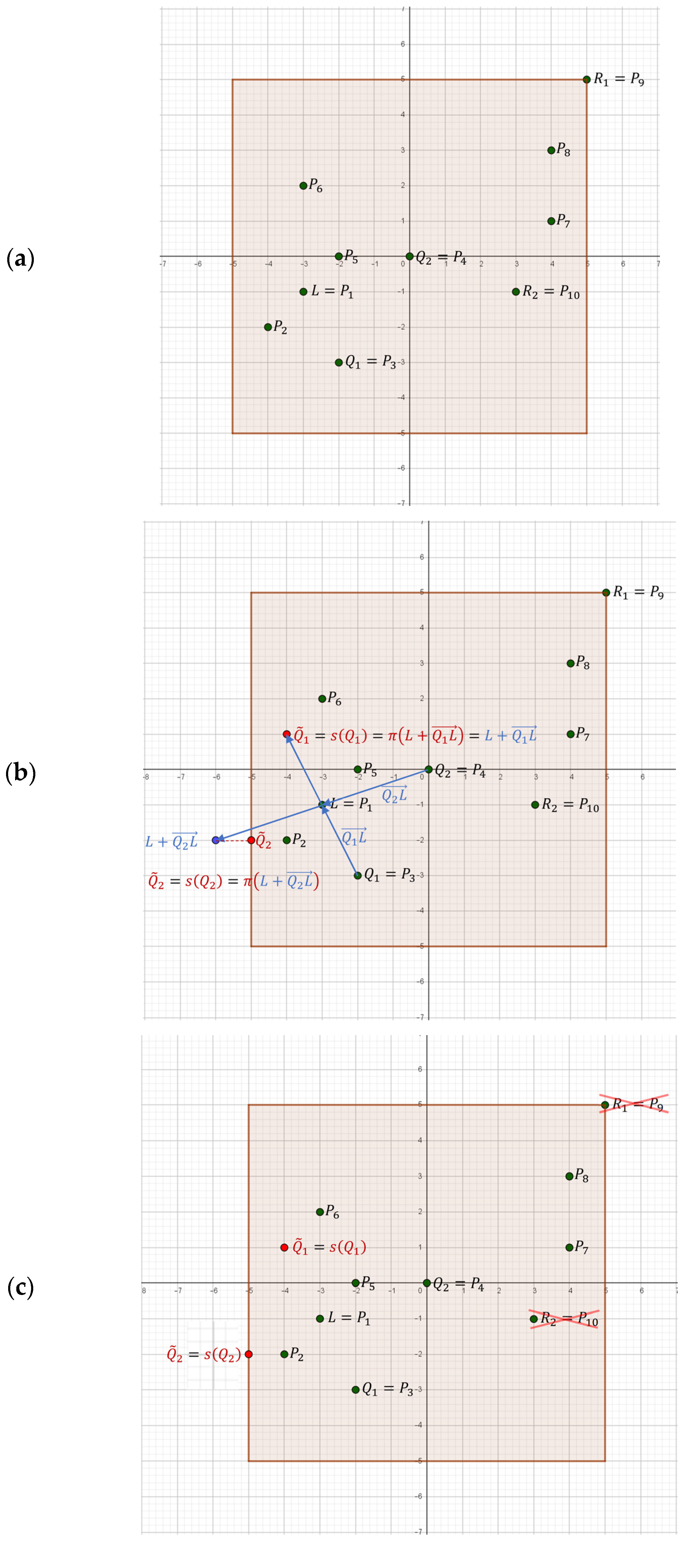
2.3. Genetic Algorithm with Symmetrization Operator (GASO)

The proposed GASO algorithm is a memetic algorithm—some transformation (symmetrization) is performed on the population of points obtained in the genetic step. Then this modified population is transferred to the next iteration of the genetic procedure. Therefore, the structure of the GASO algorithm is as follows (Algorithm 4):
Algorithm 4 Memetic algorithm in GA framework with symmetrization operator
1create random initial population: initialPopulatioIndividuals;
2compute values of objective function: initialPopulatioValues;
3while stopping criterion is NOT satisfied do
4  [nextPopulationIndividuals, nextPopulationValues] =
  stepGA(initialPopulationIndividuals, initialPopulationValues,…
   optionsOfGA, objectiveFunction);
5
6  [initialPopulationIndividuals, initialPopulatioValues] =…
7   symmetrization(nextPopulationIndividuals,…
   nextPopulationValues, objectiveFunction);
8
9end
Let us assume that after the genetic step we obtained population P of K = [ a , a ] D cube points.
P = ( P 1 ,   P 2 ,   ,   P N )
N = 100 D
Let the population P be ordered, i.e.,
f ( P 1 ) f ( P 2 )   f ( P N )
f : K function that undergoes minimization, and L = P 1 is the leader of the population P .
Definition 4 (population collapse index). 
Let
I = { i = 2 ,   3 ,   ,   N : f ( P i ) f ( L ) > ϵ }
c o l ( P ) —the collapse index for the population P is a number defined for each population P as follows
col ( P ) = { min I ,     I N ,     I =
We will call a population the collapsed one when col ( P ) > 20 D ( 20 D = 20 % of the population size). It has been experimentally found that further f symmetrization does not improve the optimization efficiency for the collapsed population. Therefore, if the population collapses, the symmetrization operation is no longer applied and P in an unchanged form is being transferred to the next genetic step.
Let k = col ( P ) 20 D , l = 15 D ( 15 D = 15 % of the population size) and i = 1 ,   2 ,   ,   l
Q i = P k + i 1 ,   R i = P N l + i
Accordingly, the population P takes the form
P = ( P 1 ,   ,   P k 1 ,   Q 1 , ,   Q l ,   P k + l , ,   P N l ,   R 1 , ,   R l )
As a result of the procedure described later, the operation of symmetrization of the population P determines certain points Q ˜ 1 ,   ,   Q ˜ l K , and transforms population to the form:
S ( P ) = ( P 1 ,   ,   P k 1 ,   Q 1 , ,   Q l ,   P k + l ,   P N l ,   Q ˜ 1 ,   ,   Q ˜ l )
This population is then passed on to the following genetic step. It is necessary to describe the method of determining the points Q ˜ 1 ,   ,   Q ˜ l . For this purpose, the τ function has been defined as:
τ ( u ) = { u ,   | u | a a s g n ( u ) ,     | u | > a
For x = ( x 1 ,   ,   x D ) D
π ( x ) = ( τ ( x 1 ) , ,   τ ( x D ) )
The π mapping is then a projection of the D space onto the cube of K .
Definition 5 (symmetry at the cube). 
For any point x K and a fixed point y K , the symmetry in the cube K with respect to the point y is defined as a mapping s y : K K defined by the formula
s y ( x ) = π ( y + x y )
Note that when y is the internal point of the set K , then for points x close enough to y , the transformation s y is simply a central symmetry with respect to the point y .
Let L 0 = L from now on. For i = 1 , ,   l points Q ˜ i were determined as follows
{ Q ˜ i = s L i 1 ( Q i ) L i = { L i 1   ,     i f     f ( Q ˜ i ) > f ( L i 1 ) Q ˜ i ,     i f     f ( Q ˜ i ) f ( L i 1 )
The symmetrization procedure pseudocode has the following form (Algorithm 5):
Algorithm 5 Symmetrization operator
1[nextPopulationIndividuals, nextPopulationValues] =…
  Symmetrization (initialPopulationIndividuals,…
  initialPopulatioValues, objectiveFunction)
2
3  determine the current leader …
   from the population initialPopulationIndividuals;
4  select points for symmetrization; // Q 1 ,…, Q l
5  for each of the selected points
6   within the cube find the image of the point…
    in symmetry with respect to the current leader…
    as defined in (13);
7   if the obtained image is better than the current leader
8    update the current leader
9    else
11    leave the leader unchanged
12    end
13   put the found images in the current population in place…
   of the worst individuals;
14  // Q 1 , , Q l -> R 1 , , R l ; S ( P ) -> nextPopulationIndividuals
15end
The individual phases of the symmetrization operator on an exemplary two-dimensional population consisting of 10 points are presented in Figure 1.
In essence, the symmetrization operation consists of subjecting to the symmetry 15 % of the “best” points of the population, significantly different in terms of the value of the objective function from the population leader. The images of these points replace the 15 % “worst” points of the population. Note that the S ( P ) population is generally not monotonically ordered with respect to the value of the objective function. The value of 15 % was selected based on numerical experiments as approximately optimal.
Two variants of the genetic algorithm with the symmetrization operation were considered, depending on the crossover operator used (similarly to the reference algorithm):
  • GASO—with the default crossover operator (cube crossover);
  • GASOSC—with segment crossover.
As an example the function No. 10 from the BBOB benchmark [42] was used. This is an ellipsoidal function described by the formula:
f 10 ( x ) = i = 1 D 10 6 i 1 D 1 z i 2 + f opt
Its characteristic feature is elongated ellipsoidal contour lines. The 3D plot and the level plot are shown in Figure 2.
The population points over the first few generations, for the reference algorithm with segment crossover (GASC) and for the corresponding algorithm with the symmetrization operator (GASOSC), for the function No. 10 are presented in Figure 3.
It can be noticed in Figure 3b that symmetrization concentrates the population along the lowest contours of the objective function. Moreover, as it is clearly visible for generations 4 and 6, the population in the symmetrization algorithm is more evenly distributed around the leader. This enables a more effective search of the “vicinity” of the best contour lines using the segment crossover operator. Thus, the symmetrization operator in the proposed GASOSC algorithm has the features of a local search algorithm, but its main feature is the cooperation with the main (genetic) algorithm for the effective operation of the crossover operator.
Let us try to justify a bit more formally the meaning of the symmetrization operator in the discussed algorithm. Let us assume that the function f is convex on some convex surroundings of the point where the function f reaches a local (global) minimum. Let A , B be parental points that belong to that environment. For a child point C = α A + ( 1 α ) B , where α   0 ;   1 , the inequality holds:
f ( C ) α f ( A ) + ( 1 α ) f ( B )
It follows that f   ( C )   f   ( A ) or f   ( C )   f   ( B ) , i.e., the child point obtained as a result of segment crossover, is better than at least one of the parents. In the final phase of the program course (exploitation), the best points in the population are generally the points closest to the leader. Applying the symmetrization operator to these points (at the expense of the “worst” points) concentrates the population around the leader. This gives a more precise minimization of the objective function as a result of using the crossover operator after symmetrization. During the initial generations, symmetrization of points remote from the leader located in different attraction pools than the leader supports a global search, along with the crossing operation.

3. Experiments

3.1. Method of Testing the Effectiveness of Optimization Algorithms

The efficiency of the considered algorithms was tested and compared using the benchmarking technique. For this purpose, the BBOB (black box optimization benchmark) was used, which was created and used by the international research community as part of the genetic and evolutionary computation conference (GECCO). The BBOB includes [42]:
  • A set of 24 test functions divided into 5 classes according to their properties
  • Data collection procedures during the optimization process
  • Post-processing procedures that create comparative tables and charts on the basis of collected data
  • Procedure for generating a document template containing generated tables and charts
BBOB is used as a competition resolution tool between conference participants who present their optimization algorithms.
Each of the 24 test functions is parameterized. After providing the parameters, we get the so-called instance of a given function, as part of the performed test procedure D = 2 ,   3 ,   5 . The algorithm is restarted when the algorithm stop condition is met, but the assumed minimum global approximation accuracy has not been achieved. The process repeats until reaching D 10 7 objective function calculations.
As a tool for comparing the effectiveness of algorithms, the empirical cumulative distribution functions of the running time of the considered algorithms obtained in post-processing were used. The probability of optimization of the examined functions (with the ϵ error less than 10 8 ) can be read, depending on the logarithm of the number of calculations of the objective function divided by the dimension of the search space D .

3.2. Numerical Test Results

Figure 4 shows the graphs of the empirical cumulative distribution functions of the measured running time for the discussed four algorithms, averaged over the entire set of 24 BBOB benchmark test functions [42], successively for the dimensions D = 2 ,   3 ,   5 . The detailed statistical data concerning performed numerical experiments are given in Appendix A (Table A1).
Detailed analysis of cumulative distribution charts for the dimension D = 5 was performed in Figure 4.
  • Having a computing budget, e.g., 5 × 10 5 calculations of the objective function, the GA algorithm solves approx. A total of 58 % of problems (finds the global minimum for 58 % of test functions with the assumed accuracy ϵ = 10 8 ). With the same computing budget, the GASO algorithm solves 90 % of problems. So we can conclude that with the above-mentioned calculation budget, GASO is 32 percentage points more effective than GA. Illustration on the chart: green dashed lines.
  • Solving 60 % of the problems needs 5 × 10 3.7 calculations of the objective function for GASO while using GA it requires 5 × 10 5.3 function calculations. GASO requires almost 40 times less computations of the objective function than the reference GA to solve 60% of the optimization problems considered. GASO is therefore 40 times faster than GA in solving 60% of problems. Illustration on the chart: blue dotted lines.
Thus, the graphs show a qualitatively greater efficiency of the algorithm with the symmetrization operation in relation to the standard genetic algorithm. Due to the logarithmic scale in the graphs, a more accurate measurement of the difference in “optimization time” by GASO and GA seems pointless. The same phenomenon occurs in higher dimensions ( D = 10 ,   20 ,   40 ).
Additionally, a synthetic measure of the effectiveness m e of the analyzed algorithm A was introduced as the arithmetic mean of the values of the four cumulative values at the indicated points. In low dimensions ( D = 2 ,   3 ), most of the tested functions are optimized by algorithms with the symmetrization operation in the interval 3 ;   6 (interval on the axis with a logarithmic scale), while in higher dimensions, the number of calculations of the objective function value increases significantly (most of the tested functions are optimized in the interval 4 ;   7 ). Therefore, we adopt the following definition of the algorithm efficiency measure:
m e ( A ) = F ( 3 ) + F ( 4 ) + F ( 5 ) + F ( 6 ) 4 · 100 % , D = 2 , 3 F ( 4 ) + F ( 5 ) + F ( 6 ) + F ( 7 ) 4 · 100 % , D 5
The method of calculating the efficiency measure so defined is illustrated in Figure 5.
The calculated measures of effectiveness for the considered algorithms for all test functions can be found in Figure 6.
The usefulness of the symmetrization operator is especially evident for the function class f10–f14 (functions with high conditioning and unimodal). These are unimodal functions whose levels (in D = 2 ) are approximately very elongated ellipses. Figure 7 shows the measures of efficiency in this class of functions.
Additionally, it is worth noting that the GASOSC algorithm (genetic algorithm with symmetrization and segment crossover) is much more effective than GASO (genetic algorithm with symmetrization and cube crossover). Such a clear advantage of one algorithm over the other occurs only in the discussed class of functions. It also seems that symmetrization improves the exploration of the search space when the objective function has many local minima located near the global minimum (such functions in the benchmark below are the functions f3, 4, 15–19, 24 [43]).
It should be emphasized that the main contribution of this article is the symmetrization operator presented. The GASO and GASOSC algorithms mentioned in the publication constitute only a test context for examining the effectiveness of the proposed operator—therefore, they are compared only with a simple GA. The authors are working on populational metaheuristics based on the GA backbone (let’s call it Algorithm X), where one of the components is the symmetrization operator proposed in the paper. Figure 8 shows the preliminary results of the efficiency of Algorithm X with regard to the GASO and GASOSC mentioned in the work and to best2009. The best2009 algorithm won the competition at the GECCO conference in 2009 and is still a reference system for comparing optimization algorithms within the COCO (comparing continuous optimizers) platform and the related BBOB benchmark. As we can see, the working Algorithm X with a significant computing budget slightly exceeds the best2009 algorithm. GASOSC does not beat best2009, but it turns out to be almost that effective with a large amount of computation.

4. Conclusions

Poor exploitation seems to be a significant disadvantage of the classical genetic algorithm. Even if the population points are in the appropriate local extremum attraction pool, one has to wait many generations before the target subset of the search space is reached, where the minimization is carried out with an assumed error (here a very small one: ϵ = 10 8 ). The article presents the genetic algorithm with the symmetrization operator (GASO), which is a memetic modification of the classical GA, based on the idea of cyclic symmetrization of the population around the current leader. The weakest points in the search space belonging to the current population are replaced by images of some good points at central symmetry relative to the current leader. In this way, the current leader is surrounded “on all sides” with parental points, which influences the effectiveness of the crossover operators specific for optimization with constraints, in particular. The efficiency of this algorithm was tested on a set of 24 continuous functions on a multidimensional cube [43] using the recognized BBOB benchmark [42]. The advantage of the genetic algorithm with the symmetrization operator over the standard genetic algorithm turned out to be particularly visible in the class of test functions referred to in the benchmark as functions with high conditioning and unimodal [42]. These are functions whose 2D contours are very elongated ellipses. The symmetrization operator accelerates the process of grouping the population along the narrow ridge of this type of function plot. The crossover efficiency translates into the efficiency of the entire GASO algorithm. Some other tests point out that, in the case of multimodal functions, whose local minima are close to each other, the algorithm with the symmetrization operation also improves the exploration of the search space, which will be a subject of further research.

Author Contributions

Conceptualization, G.K., A.L. and J.K.; Formal analysis, A.L.; Investigation, G.K.; Project administration, J.K.; Software, G.K.; Visualization, G.K.; Writing—original draft, G.K.; Writing—review & editing, A.L. and J.K. All authors have read and agreed to the published version of the manuscript.

Funding

This research received no external funding.

Institutional Review Board Statement

Not applicable.

Informed Consent Statement

Not applicable.

Conflicts of Interest

The authors declare no conflict of interest.

Appendix A

Table A1. Expected running time (ERT in number of function evaluations) on functions f1, f2, …, f24 in dimension 5 divided by the best ERT measured during BBOB-2009. The ERT and in braces, as dispersion measure, the half difference between 90 and 10% tile of bootstrapped run lengths appear in the second row of each cell, the best ERT in the first. The different target ∆f values are shown in the top row. #succ is the number of trials that reached the (final) target f o p t + 10 8 . The median number of conducted function evaluations is additionally given in italics, if the target in the last column was never reached. Bold entries are more statistically significantly (according to the rank-sum test) compared to the best algorithm in BBOB-2009, with p = 0.05 or p = 10 k when the number k > 1 is following the ↓ symbol, with Bonferroni correction by the number of functions.
fopt1 × 1011 × 1001 × 10−11 × 10−21 × 10−31 × 10−51 × 10−7#Succ
f11112121212121215/15
GA6.5 (20)83 (39)184 (48)321 (83)465 (130)872 (335)2132 (1127)15/15
GASC12 (14)89 (47)225 (120)427 (185)742 (371)1494 (624)1.1 × 10⁴ (6256)15/15
GASO7.1 (5)82 (19)182 (27)274 (24)376 (29)561 (32)756 (40)15/15
GASOSC11 (18)99 (33)177 (54)253 (66)347 (51)527 (71)719 (51)15/15
f28387888990929415/15
GA68 (21)98 (25)128 (31)158 (38)196 (60)302 (58)1258 (176)15/15
GASC93 (27)139 (48)185 (96)237 (90)289 (84)445 (277)6240 (2 × 10⁴)15/15
GASO44 (4)55 (6)68 (6)81 (8)92 (4)117 (7)137 (5)15/15
GASOSC44 (12)56 (8)70 (4)79 (9)92 (6)116 (9)135 (8)15/15
f371616221637164216461650165415/15
GA4.2 (0.9)8.9 (4)11 (5)13 (5)16 (4)23 (7)96 (162)15/15
GASC4.2 (0.9)11 (5)14 (7)17 (4)20 (7)30 (6)535 (977)14/15
GASO4.7 (2)6.6 (3)8.5 (2)9.0 (5)9.5 (3)11 (2)12 (3)15/15
GASOSC4.7 (2)8.0 (2)9.4 (4)10 (4)11 (3)13 (3)15 (5)15/15
f480916331688175818171886190315/15
GA5.7 (1)9 (5)24 (7)25 (8)27 (10)35 (7)2555 (3222)9/15
GASC6.5 (2)19 (4)27 (17)29 (4)31 (7)38 (11)1571 (1730)11/15
GASO5.1 (2)13 (4)25 (16)25 (17)24 (22)25 (14)25 (17)15/15
GASOSC5.2 (0.9)19 (5)29 (9)29 (10)29 (12)29 (16)30 (14)15/15
f51010101010101015/15
GA401 (89)2212 (826)1.9 × 10⁴ (3 × 10⁴)1.0 × 10⁶ (5 × 10⁵)7.2 × 10⁶ (9 × 10⁶) 0/15
GASC400 (178)1531 (601)2566 (475)4370 (812)7246 (4763)2.4 × 10⁵ (4 × 10⁵)3.3 × 10⁶ (5 × 10⁶)2/15
GASO106 (4)125 (30)125 (58)125 (31)125 (31)125 (59)125 (58)15/15
GASOSC112 (27)132 (28)132 (42)132 (57)132 (28)132 (28)132 (57)15/15
f61142142814045801038133215/15
GA13 (5)31 (12)68 (32)99 (53)109 (14)2600 (1752)5.3 × 10⁴ (6 × 10⁴)1/15
GASC14 (4)36 (15)80 (27)114 (56)127 (53)1603 (1401)2.5 × 10⁴ (4 × 10⁴)2/15
GASO13 (6)19 (4)25 (5)26 (4)24 (3)19 (2)20 (1)15/15
GASOSC12 (3)18 (4)35 (41)43 (10)43 (43)54 (41)155 (203)15/15
f7243241171145115721572159715/15
GA28 (11)7.7 (2)12 (18)15 (16)17 (15)17 (26)18 (8)15/15
GASC23 (16)5.6 (3)14 (11)38 (45)44 (66)44 (41)44 (34)15/15
GASO26 (18)5.8 (2)3.0 (0.4)3.5 (0.5)3.5 (0.5)3.5 (0.5)3.9 (0.7)15/15
GASOSC29 (10)5.7 (1)2.8 (1)3.3 (0.4)3.2 (0.5)3.2 (1.0)3.5 (0.7)15/15
f87327333637239141042215/15
GA32 (12)117 (92)554 (164)1.1 × 10⁴ (1 × 10⁴)5.7 × 10⁴ (4 × 10⁴)∞5.0 × 1060/15
GASC30 (4)86 (41)392 (175)6584 (6838)2.0 × 10⁴ (2 × 10⁴)∞5.0 × 1060/15
GASO30 (6)35 (3)39 (23)44 (38)50 (35)63 (7)73 (30)15/15
GASOSC26 (4)23 (15)27 (13)30 (18)32 (6)37 (13)41 (16)15/15
f93512721426330033536915/15
GA67 (8)959 (2533)1.1 × 10⁵ (8 × 10⁴)∞5.0 × 1060/15
GASC58 (10)503 (550)2.2 × 10⁴ (3 × 10⁴)1.4 × 10⁵ (65855)2.5 × 10⁵ (5 × 10⁵)∞5.0 × 1060/15
GASO55 (22)48 (10)49 (14)49 (14)56 (15)70 (14)83 (20)15/15
GASOSC54 (11)55 (62)48 (44)46 (37)45 (17)47 (14)49 (23)15/15
f1034950057460762682988015/15
GA1478 (747)5129 (5387)58957 (59058)1.2 × 10⁵ (1 × 10⁵)∞5.0 × 1060/15
GASC2278 (1784)4693 (573)61284 (84901)1.2 × 10⁵ (1 × 10⁵)∞5.0 × 1060/15
GASO31 (20)37 (16)53 (25)64 (19)80 (21)119 (106)1700 (3161)14/15
GASOSC13 (2)12 (313 (2)14 (1)15 (2014 (2)16 (2)15/15
f1114320276397711771467167315/15
GA494 (1263)5235 (16,771)7703 (11,197)21,366 (24,263)∞5.0 × 1060/15
GASC88 (232)1617 (4927)1597 (738)2490 (2527)10,664 (11340)∞5.0 × 1060/15
GASO27 (20)45 (16)20 (8)21 (6)22 (6)27 (7)108 (222)14/15
GASOSC14 (5)18 (2)6.4 (1)6.3 (1)6.2 (1)6.4 (0.5)6.9 (0.6)15/15
f121082683714134611303149415/15
GA84 (18)1088 (1044)2476 (4365)3819 (2294)9005 (9476)5.5 × 10⁴ (7 × 10⁴)∞5.0 × 1060/15
GASC482 (851)1396 (317)2538 (2599)4290 (2636)9784 (1 × 10⁴)∞5.0 × 1060/15
GASO151 (69)131 (41)159 (91)177 (203)208 (174)213 (401)3375 (2673)8/15
GASOSC69 (3)57 (49)61 (67)67 (53)69 (46)31 (13)36 (23)15/15
f1313219525031913101752225515/15
GA171 (512)2378 (429)7002 (6945)8492 (2 × 10⁴)3577 (4272)2.0 × 10⁴ (2 × 10⁴)∞5.0 × 1060/15
GASC58 (90)2260 (530)3585 (7272)6755 (8523)4206 (3977)2.0 × 10⁴ (1 × 10⁴)∞5.0 × 1060/15
GASO30 (6)41 (8)54 (8)111 (84)61 (92)394 (454)4024 (4054)6/15
GASOSC24 (6)26 (2)29 (2)31 (2)9.2 (2)9.3 (2)9.1 (0.9)145/15
f141041589013925147615/15
GA1.7 (1)24 (3)43 (10)49 (15)74 (65)6913 (14125)∞5.0 × 1060/15
GASC1.4 (5)21 (841 (8)52 (11)100 (61)12530 (17044)∞5.0 × 1060/15
GASO1.7 (5)19 (5)38 (3)40 (4)42 (5)62 (12)1084 (1057)2/15
GASOSC1.5 (2)17 (13)35 (10)39 (7)35 (5)33 (3)24 (1)15/15
f155931019,36919,74320,07320,76921,35914/15
GA7.5 (2)26 (77)78 (86)77 (21)76 (82)105 (128)1672 (2443)2/15
GASC6.1 (0.9)37 (63)125 (156)123 (131)122 (51)167 (320)1600 (1405)2/15
GASO8.0 (2)9.1 (10)14 (16)14 (16)14 (15)13 (16)13 (8)15/15
GASOSC6.1 (3)14 (24)57 (55)56 (47)55 (36)53 (34)52 (34)15/15
f16120612266310,16310,44911,64412,09515/15
GA3.0 (3)22 (4)19 (17)14 (20)109 (157)1042 (1505)1285 (232)2/15
GASC3.1 (2)15 (30)35 (51)28 (27)110 (161)851 (1503)∞5.0 × 1060/15
GASO2.8 (2)8.7 (2)8.9 (7)3.4 (6)3.8 (5)4.3 (5)4.4 (3)15/15
GASOSC3.2 (3)16 (15)12 (8)4.8 (6)6.4 (6)10 (19)10 (18)15/15
f175.2215899286136696351793415/15
GA3.7 (2)7.9 (3)7.1 (3)31 (38)109 (161)1164 (1396)∞5.0 × 1060/15
GASC3.2 (3)8.2 (5)47 (23)61 (54)261 (362)∞5.0 × 1060/15
GASO2.5 (5)7.6 (2)5.3 (0.9)2.6 (0.1)3.0 (0.3)3.3 (0.3)4.8 (1)15/15
GASOSC3.3 (3)7.4 (2)4.7 (1)3.7 (4)10 (11)19 (23)94 (107)15/15
f1810337839688451928010,90512,46915/15
GA6.4 (3)10 (3)16 (22)74 (46)353 (730)3323 (3210)∞5.0 × 1060/15
GASC6.6 (3)12 (2)25 (9)291 (524)3882 (6186)∞5.0 × 1060/15
GASO7.3 (6)9.3 (1)3.5 (1)5.2 (6)10 (13)30 (52)92 (190)12/15
GASOSC6.3 (3)8.3 (2)3.2 (0.4)5.9 (5)18 (17)100 (135)172 (145)12/15
f19112421.0 × 1051.2 × 1051.2 × 1051.2 × 10515/15
GA55 (137)1995 (665)302 (618)148 (107)278 (507)588 (743)∞5.0 × 1060/15
GASC46 (61)2572 (1246)427 (676)32 (21)205 (198)307 (433)613 (625)1/15
GASO15 (9)2955 (1240)162 (165)15 (30)47 (66)46 (42)46 (59)9/15
GASOSC17 (28)2853 (828)147 (184)23 (20)41 (61)41 (81)41 (58)9/15
f201685138,11151,36254,47054,86155,31314/15
GA14 (18)8.5 (3)4.7 (7)3.6 (6)3.5 (8)4.9 (8)41 (63)7/15
GASC22 (16)14 (23)17 (13)12 (7)12 (5)12 (9)78 (151)4/15
GASO26 (13)7.5 (6)3.8 (4)2.9 (1)2.7 (4)2.7 (1)2.8 (1)15/15
GASOSC22 (17)15 (10)13 (19)10 (9)9.4 (3)9.4 (2)9.4 (15)15/15
f21411157167416921701729175714/15
GA4.2 (4)6.4 (7)6.5 (9)7.7 (10)9.4 (12)15 (15)46 (32)15/15
GASC1.9 (2)17 (24)13 (22)14 (8)16 (19)26 (20)43 (23)15/15
GASO3.0 (5)2.8 (6)4.3 (7)4.6 (7)4.9 (7)5.7 (7)6.4 (0.5)15/15
GASOSC2.9 (3)2.8 (1.0)6.0 (7)6.3 (8)6.6 (7)7.1 (4)7.7 (8)15/15
f227138693898010081040106814/15
GA5.1 (6)10 (21)10 (13)19 (14)35 (32)199 (220)1072 (373)11/15
GASC5.2 (6)5.3 (11)9.3 (18)12 (9)19 (39)187 (347)1290 (1961)13/15
GASO5.6 (4)4.6 (0.8)13 (13)13 (23)14 (23)15 (22)17 (2)15/15
GASOSC4.2 (4)12 (31)7.5 (13)8.7 (12)9.2 (18)10 (9)11 (18)15/15
f233.0518142492789031654330303425615/15
GA2.0 (2)14 (7)16 (17)203 (242)1103 (1406)∞5.0 × 1060/15
GASC1.9 (1)11 (3)27 (43)192 (357)2296 (1027)∞5.0 × 1060/15
GASO2.5 (3)10 (6)2.8 (2)1.7 (3)1.6 (2)1.8 (2)1.9 (2)15/15
GASOSC1.9 (0.8)11 (4)7.9 (10)7.4 (9)6.8 (9)11 (13)13 (12)15/15
f2416222.2 × 1056.4 × 1069.6 × 1069.6 × 1061.3 × 1071.3 × 1073/15
GA4.3 (2)25 (26)∞5.0 × 1060/15
GASC3.4 (0.8)47 (30)∞5.0 × 1060/15
GASO4.3 (2)23 (36)∞5.0 × 1060/15
GASOSC2.9 (0.8)12 (8)∞5.0 × 1060/15

References

  1. Boussaïd, I.; Lepagnot, J.; Siarry, P. A survey on optimization metaheuristics. Inf. Sci. 2013, 237, 82–117. [Google Scholar] [CrossRef]
  2. Kirkpatrick, S.; Gelatt, C.D., Jr.; Vecchi, M.P. Optimization by Simulated Annealing. Science 1983, 220, 671–680. [Google Scholar] [CrossRef]
  3. Glover, F. Paths for Integer Programming. Comput. Oper. Res. 1986, 13, 533–549. [Google Scholar]
  4. Mladenović, N.; Dražić, M.; Kovačevic-Vujčić, V.; Čangalović, M. General variable neighborhood search for the continuous optimization. Eur. J. Oper. Res. 2008, 191, 753–770. [Google Scholar] [CrossRef]
  5. Voudouris, C. Guided Local Search—An Illustrative Example in Function Optimisation. BT Technol. J. 1998, 16, 46–50. [Google Scholar] [CrossRef]
  6. Stutzle, T.G. Local Search Algorithms for Combinatorial Problems. Ph.D. Thesis, Darmstadt University of Technology, Darmstadt, Germany, 1998. [Google Scholar]
  7. Holland, J.H. Adaptation in Natural and Artificial Systems, 1st ed.; University of Michigan Press: Ann Arbor, MI, USA, 1975. [Google Scholar]
  8. Rechenberg, I. Evolution Strategy: Nature’s Way of Optimization. In Optimization: Methods and Applications, Possibilities and Limitations; Springer: Berlin/Heidelberg, Germany, 1989; pp. 106–126. [Google Scholar] [CrossRef]
  9. Koza, J.R. Genetic programming as a means for programming computers by natural selection. Stat. Comput. 1994, 4, 87–112. [Google Scholar] [CrossRef]
  10. Storn, R.; Price, K. Differential evolution—A simple and efficient heuristic for global optimization over continuous spaces. J. Glob. Optim. 1997, 11, 341–359. [Google Scholar] [CrossRef]
  11. Reynolds, R.G. An introduction to cultural algorithms. In Proceedings of the Third Annual Conference on Evolutionary Programming, San Diego, CA, USA, 24–26 February 1994; pp. 131–139. [Google Scholar]
  12. Dorigo, M.; Maniezzo, V.; Colorni, A.; Dorigo, M. Positive Feedback as a Search Strategy. Technical Report 91-016. 1991. pp. 1–20. Available online: http://citeseerx.ist.psu.edu/viewdoc/summary?doi=10.1.1.52.6342 (accessed on 1 April 2022).
  13. Kennedy, J.; Eberhart, R. Particle Swarm Optimization. In Proceedings of the ICNN’95—International Conference on Neural Networks, Perth, Australia, 27 November–1 December 1995; Volume 4, pp. 1942–1948. [Google Scholar] [CrossRef]
  14. Karaboga, D.; Akay, B. A survey: Algorithms simulating bee swarm intelligence. Artif. Intell. Rev. 2009, 31, 61–85. [Google Scholar] [CrossRef]
  15. Timmis, J.; Andrews, P.; Owens, N.; Clark, E. An interdisciplinary perspective on artificial immune systems. Evol. Intell. 2008, 1, 5–26. [Google Scholar] [CrossRef] [Green Version]
  16. Talbi, E.-G. Machine Learning into Metaheuristics. ACM Comput. Surv. 2022, 54, 1–32. [Google Scholar] [CrossRef]
  17. Katoch, S.; Chauhan, S.S.; Kumar, V. A review on genetic algorithm: Past, present, and future. Multimed. Tools Appl. 2021, 80, 8091–8126. [Google Scholar] [CrossRef] [PubMed]
  18. Lee, C. A review of applications of genetic algorithms in operations management. Eng. Appl. Artif. Intell. 2018, 76, 1–12. [Google Scholar] [CrossRef]
  19. Hiassat, A.; Diabat, A.; Rahwan, I. A genetic algorithm approach for location-inventory-routing problem with perishable products. J. Manuf. Syst. 2017, 42, 93–103. [Google Scholar] [CrossRef]
  20. Kaur, M.; Kumar, V. Parallel non-dominated sorting genetic algorithm-II-based image encryption technique. Imaging Sci. J. 2018, 66, 453–462. [Google Scholar] [CrossRef]
  21. Wolpert, D.H.; Macready, W.G. No free lunch theorems for optimization. IEEE Trans. Evol. Comput. 1997, 1, 67–82. [Google Scholar] [CrossRef] [Green Version]
  22. Wright, A.H. Genetic Algorithms for Real Parameter Optimization. In Foundations of Genetic Algorithms; Elsevier: Amsterdam, The Netherlands, 1991; pp. 205–218. [Google Scholar] [CrossRef]
  23. Michalewicz, Z. Genetic Algorithms + Data Structures = Evolution Programs; Springer: Berlin/Heidelberg, Germany, 1996. [Google Scholar]
  24. Chuang, Y.-C.; Chen, C.-T.; Hwang, C. A simple and efficient real-coded genetic algorithm for constrained optimization. Appl. Soft Comput. 2016, 38, 87–105. [Google Scholar] [CrossRef]
  25. Das, A.K.; Pratihar, D.K. A Direction-Based Exponential Crossover Operator for Real-Coded Genetic Algorithm. In Recent Advances in Theoretical, Applied, Computational and Experimental Mechanics; Springer: Singapore, 2020; pp. 311–323. [Google Scholar]
  26. Ono, I.; Kita, H.; Kobayashi, S. A Real-coded Genetic Algorithm using the Unimodal Normal Distribution Crossover. In Advances in Evolutionary Computing; Springer: Berlin/Heidelberg, Germany, 2003; pp. 213–237. [Google Scholar]
  27. Deep, K.; Thakur, M. A new crossover operator for real coded genetic algorithms. Appl. Math. Comput. 2007, 188, 895–911. [Google Scholar] [CrossRef]
  28. Das, A.K.; Pratihar, D.K. A Direction-Based Exponential Mutation Operator for Real-Coded Genetic Algorithm. In Proceedings of the 2018 Fifth International Conference on Emerging Applications of Information Technology (EAIT), Kolkata, India, 12–13 January 2018; pp. 1–4. [Google Scholar] [CrossRef]
  29. Tang, P.-H.; Tseng, M.-H. Adaptive directed mutation for real-coded genetic algorithms. Appl. Soft Comput. 2013, 13, 600–614. [Google Scholar] [CrossRef]
  30. Hussain, A.; Muhammad, Y.S. Trade-off between exploration and exploitation with genetic algorithm using a novel selection operator. Complex Intell. Syst. 2020, 6, 1–14. [Google Scholar] [CrossRef] [Green Version]
  31. Chen, J.-C.; Cao, M.; Zhan, Z.-H.; Liu, D.; Zhang, J. A New and Efficient Genetic Algorithm with Promotion Selection Operator. In Proceedings of the 2020 IEEE International Conference on Systems, Man, and Cybernetics (SMC), Toronto, ON, Canada, 11–14 October 2020; pp. 1532–1537. [Google Scholar] [CrossRef]
  32. Espinoza, F.P.; Minsker, B.; Goldberg, D.E. Performance Evaluation and Population Reduction for a Self Adaptive Hybrid Genetic Algorithm (SAHGA). Lect. Notes Comput. Sci. 2003, 2723, 922–933. [Google Scholar] [CrossRef]
  33. Elmihoub, T.; Hopgood, A.A.; Nolle, L.; Battersby, A. Performance of hybrid genetic algorithms incorporating local search. In Proceedings of the 18th European Simulation Multiconference, Nottingham, UK, 13–16 June 2004; Volume 4, pp. 154–160. Available online: http://scs-europe.net/services/esm2004/pdf/esm-56.pdf (accessed on 1 April 2022).
  34. Konak, A.; Smith, A. A hybrid genetic algorithm approach for backbone design of communication networks. In Proceedings of the 1999 Congress on Evolutionary Computation-CEC99 (Cat. No. 99TH8406), Washington, DC, USA, 6–9 July 1999; Volume 3, pp. 1817–1823. [Google Scholar] [CrossRef]
  35. Hedar, A.-R.; Fukushima, M. Simplex Coding Genetic Algorithm for the Global Optimization of Nonlinear Functions. In Multi-Objective Programming and Goal Programming; Springer: Berlin/Heidelberg, Germany, 2003; pp. 135–140. [Google Scholar]
  36. Chaiyaratana, N.; Zalzala, A.M.S. Hybridisation of neural networks and a genetic algorithm for friction compensation. In Proceedings of the 2000 Congress on Evolutionary Computation. CEC00 (Cat. No. 00TH8512), La Jolla, CA, USA, 16–19 July 2000; Volume 1, pp. 22–29. [Google Scholar] [CrossRef]
  37. Neri, F.; Cotta, C. Memetic algorithms and memetic computing optimization: A literature review. Swarm Evol. Comput. 2012, 2, 1–14. [Google Scholar] [CrossRef]
  38. Goldberg, D.E. Genetic Algorithms in Search, Optimization, and Machine Learning; Addison-Wesley Longman Publishing Co., Inc.: Boston, MA, USA, 1989. [Google Scholar]
  39. Dawkins, R. The Selfish Gene: 30th Anniversary Edition; Oxford University Press: Oxford, UK, 2006; Volume 214. [Google Scholar]
  40. Norman, M.G.; Moscato, P. A Competitive-Cooperative Approach to Complex Combinatorial Search. In Proceedings of the 20th Informatics and Operations Research Meeting, July 1999; pp. 15–29. Available online: http://citeseerx.ist.psu.edu/viewdoc/download?doi=10.1.1.44.776&rep=rep1&type=pdf (accessed on 1 April 2022).
  41. Hart, W.E.; Krasnogor, N.; Smith, J.E. Memetic Evolutionary Algorithms. In Recent Advances in Memetic Algorithms; Springer: Berlin/Heidelberg, Germany, 2006; pp. 3–27. [Google Scholar]
  42. Hansen, N.; Auger, A.; Finck, S.; Ros, R. Real-Parameter Black-Box Optimization Benchmarking BBOB-2010: Experimental Setup; INRIA Research Report; INRIA: Le Chesnay-Rocquencourt, France, 2010; pp. 1–18. Available online: http://citeseerx.ist.psu.edu/viewdoc/download?doi=10.1.1.168.5204&rep=rep1&type=pdf (accessed on 1 April 2022).
  43. Finck, S.; Ros, R. Real-Parameter Black-Box Optimization Benchmarking 2010: Noiseless Functions Definitions. 2010. pp. 1–12. Available online: http://coco.gforge.inria.fr/bbob2010-downloads (accessed on 1 April 2022).
Figure 1. Successive stages of the symmetrization operator on an example population consisting of 10 points. (a) In the population sorted by the value of the objective function, the leader was distinguished ( L = P 1 ), points collapsed with the leader ( P 2 ), points selected for symmetrization ( Q 1 = P 3 ,   Q 2 = P 4 ), the remaining points are not a subject to any modifications ( P 5 , P 6 , P 7 , P 8 ), the “worst” points due to the values of the objective function ( R 1 = P 9 , R 2 = P 10 ). (b) For points Q 1 ,   Q 2 their images were found Q ˜ 1 ,   Q ˜ 2 using the described symmetrization operator; on Q ˜ 2 it was necessary to use the cube projection operator. (c) The “worst” points were removed from the population; R 1 , R 2 were replaced with points resulting from the symmetrization operator Q ˜ 1 ,   Q ˜ 2 .
Applsci 12 05426 g001
Figure 2. The ellipsoidal function, function no. 10 from the benchmark. 2D plots: surface (a) and level (b). Black arrow indicates the optimal point of the function.
Applsci 12 05426 g002
Figure 3. The scattering of points (black dots) in the search space in several initial generations (in consecutive rows) for the reference algorithm with segment crossover—GASC (column (a)) and for the corresponding algorithm with the symmetrization operator—GASOSC (column (b)) on the example of function No. 10 from the set of test functions from BBOB benchmark in dimension 2. Color lines show the contours of the function.
Applsci 12 05426 g003
Figure 4. Empirical cumulative distribution functions of the measured runtime (the number of calculations of the objective functions divided by dimension of search space) for four algorithms averaged for the entire set of 24 test functions of the BBOB benchmark successively for dimensions 2 (a), 3 (b) and 5 (c). The considered algorithms are: GA—reference generic algorithm with standard crossover, GASC—reference genetic algorithm with segment crossover, GASO—genetic algorithm with symmetrization operator and standard crossover, GASOSC—genetic algorithm with symmetrization operator and segment crossover.
Applsci 12 05426 g004
Figure 5. The method of converting the values read from the graph of the empirical cumulative distribution function of operating time measured with the number of objective function calculations for the GASOSC algorithm, averaged for the entire set of 24 test functions of the BBOB benchmark for dimension 5 into a synthetic measure of the algorithm effectiveness me according to the given formula. The considered algorithm is GASOSC—a genetic algorithm with a symmetrization operator and segment crossover.
Applsci 12 05426 g005
Figure 6. Synthetic measures of effectiveness for the four considered algorithms for dimensions 2 (a), 3 (b) and 5 (c) for the entire set of 24 test functions of the BBOB benchmark calculated as presented in Figure 5. The considered algorithms are: GA—reference generic algorithm with standard crossover, GASC—reference genetic algorithm with segment crossover, GASO—genetic algorithm with symmetrization operator and standard crossover, GASOSC—genetic algorithm with symmetrization operator and segment crossover.
Applsci 12 05426 g006
Figure 7. Synthetic measures of effectiveness for the four considered algorithms for dimensions 2 (a), 3 (b) and 5 (c) for the five from 24 test functions defined as functions with high conditioning and unimodal of the BBOB benchmark calculated as presented in Figure 5. The considered algorithms are: GASt—reference generic algorithm with standard crossover, GASC—reference genetic algorithm with segment crossover, GASO—genetic algorithm with symmetrization operator and standard crossover, GASOSC—genetic algorithm with symmetrization operator and segment crossover.
Applsci 12 05426 g007
Figure 8. Empirical cumulative distribution functions of the measured runtime (the number of calculations of the objective functions divided by dimension of search space) for four algorithms aver-aged for the entire set of 24 test functions of the BBOB benchmark for dimensions 5. The considered algorithms are: GASC—reference genetic algorithm with segment crossover, GASOSC—genetic algorithm with symmetrization operator and segment crossover, best2009—the reference algorithm on the COCO platform of which BBOB is a part (winner of the 2009 GECCO competition)—still in use.
Applsci 12 05426 g008
Publisher’s Note: MDPI stays neutral with regard to jurisdictional claims in published maps and institutional affiliations.

