
Dynamic Energy Efficient Control of Induction Machines Using Anticipative Flux Templates


Abstract
:1. Introduction
2. Modeling
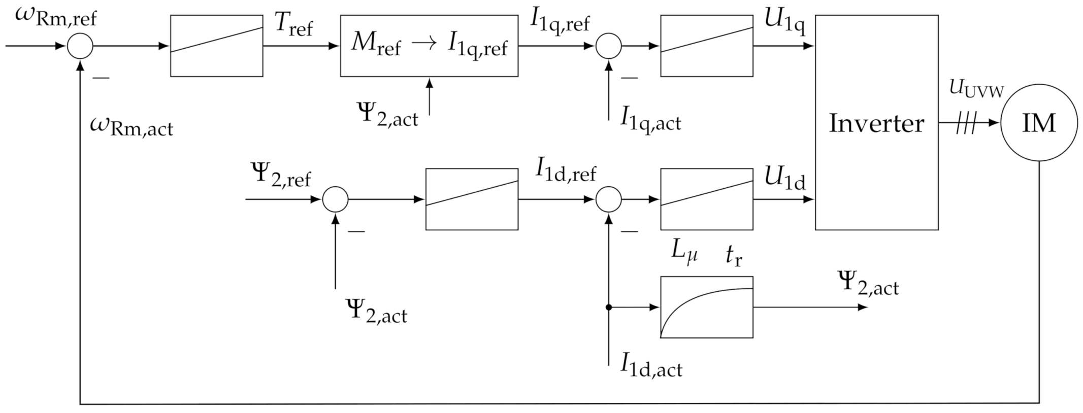
2.1. Machine Model
2.2. Main Inductance Saturation
2.3. Loss Model
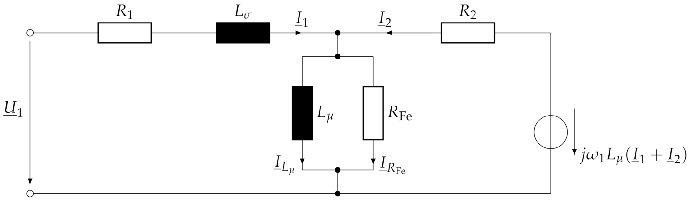
2.4. Influence of Iron Losses
3. Optimization Procedure
3.1. Optimal Control Problem
3.2. Implementation
3.3. Optimal Offline Solution
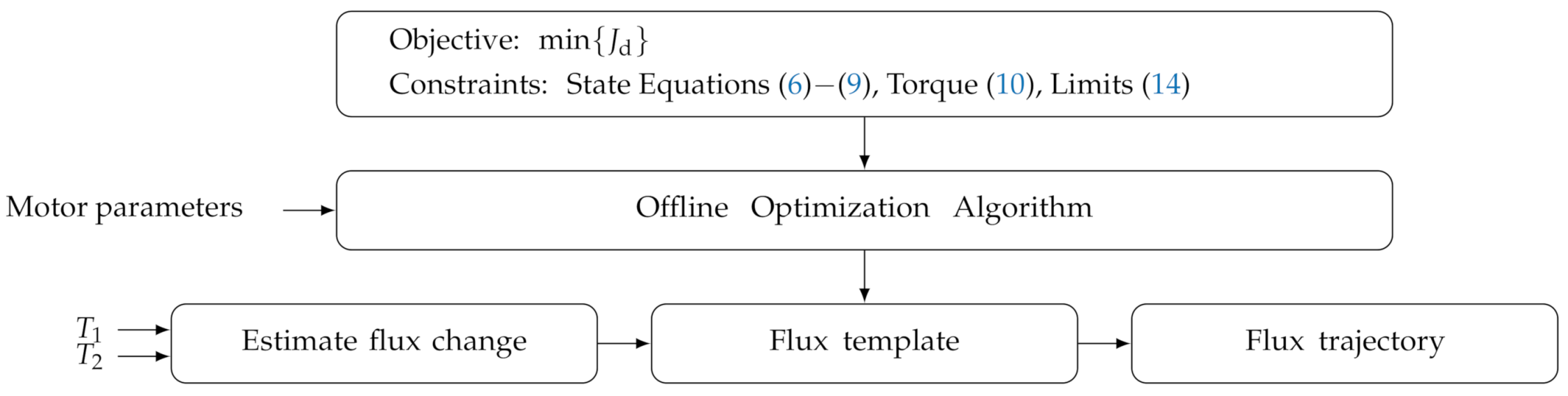
4. Template Based Solution
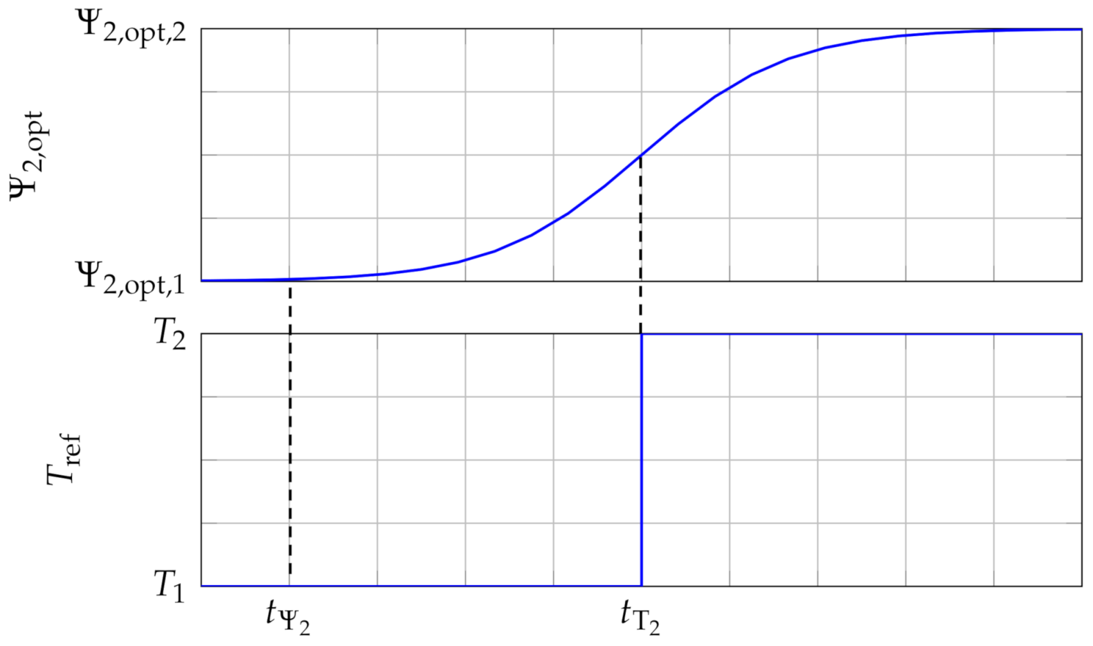
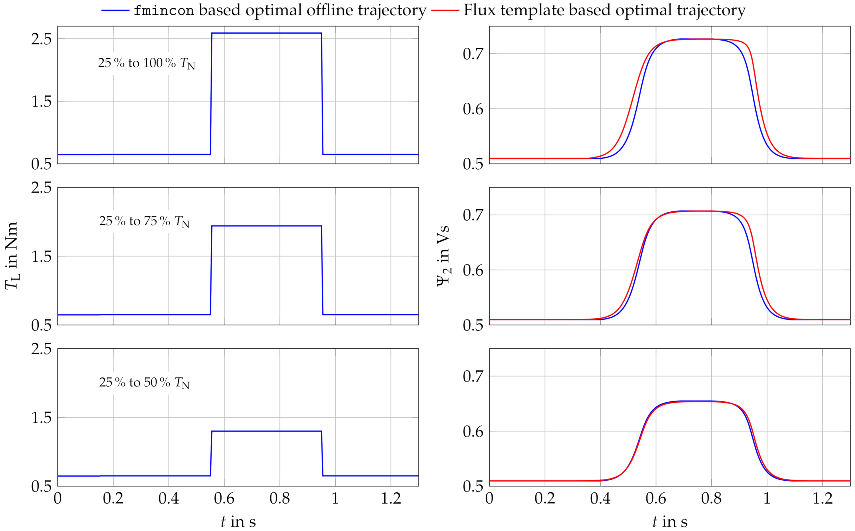
4.1. Template Generation
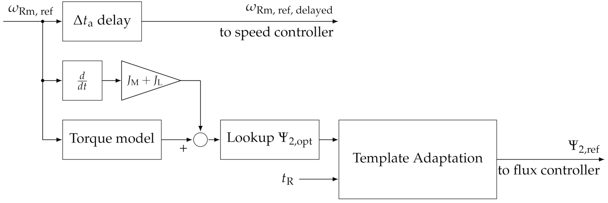
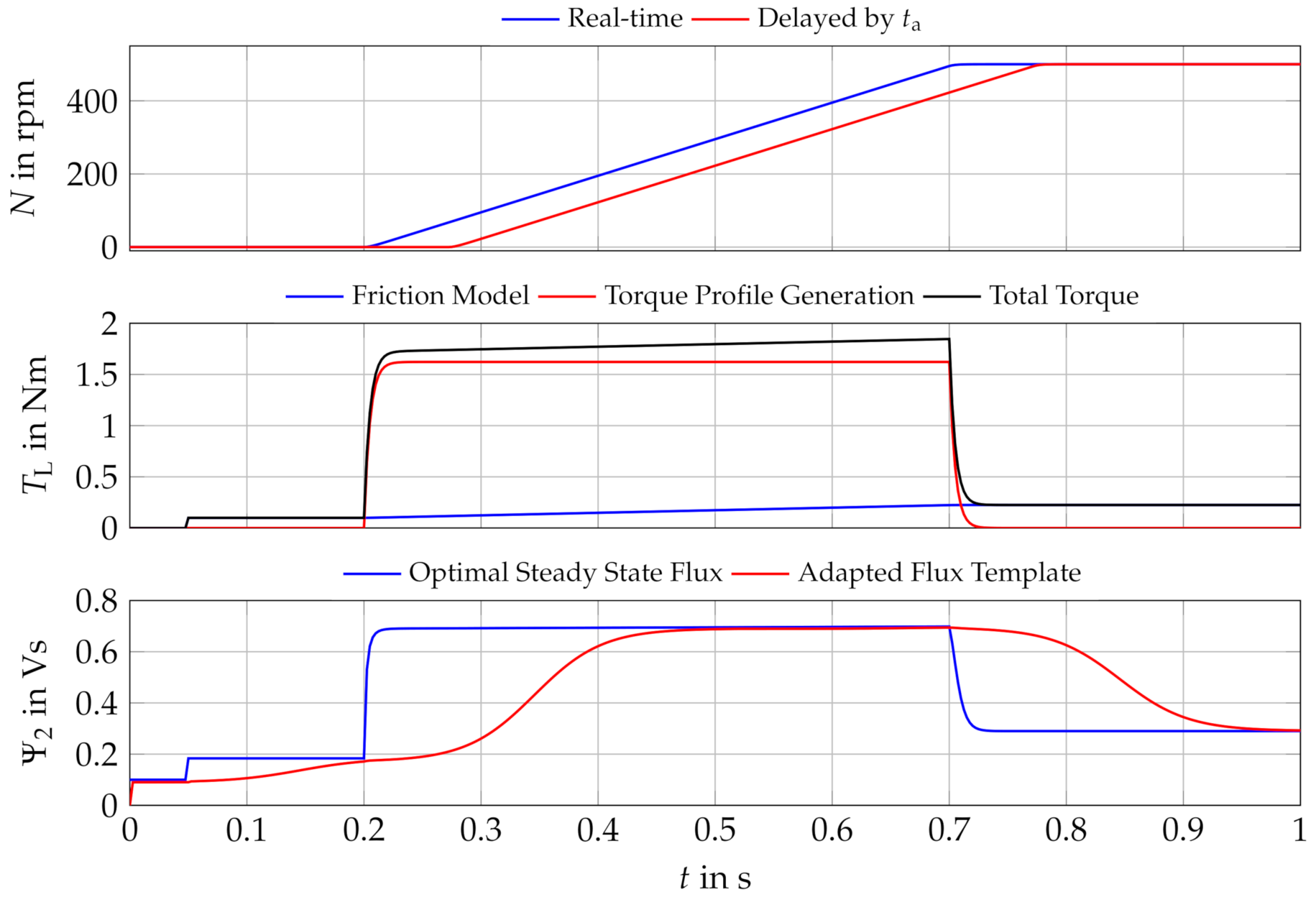
4.2. Template Adaptation
5. Model Predictive Solution
6. Simulations
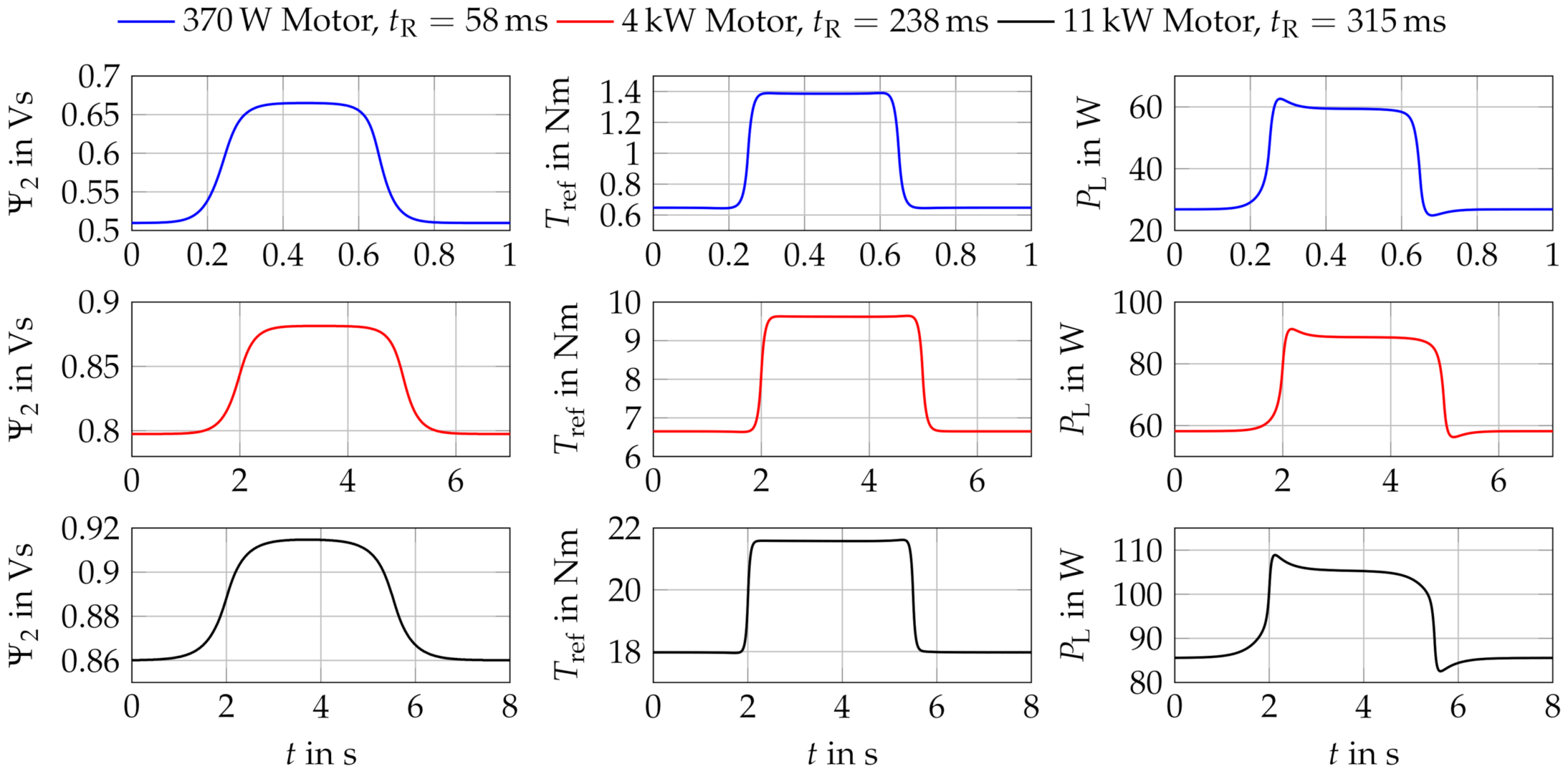
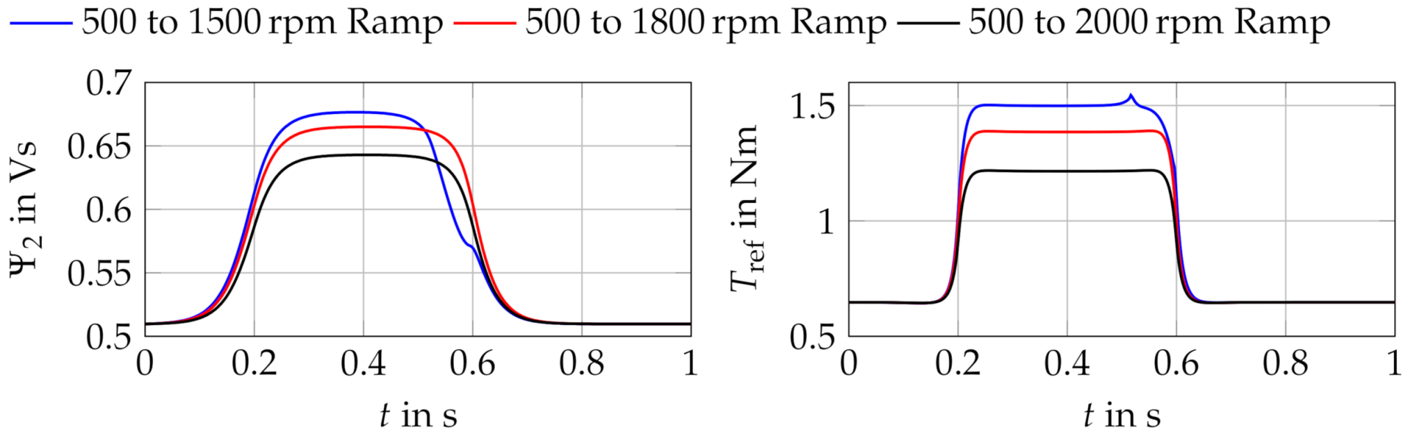
6.1. Template Generation
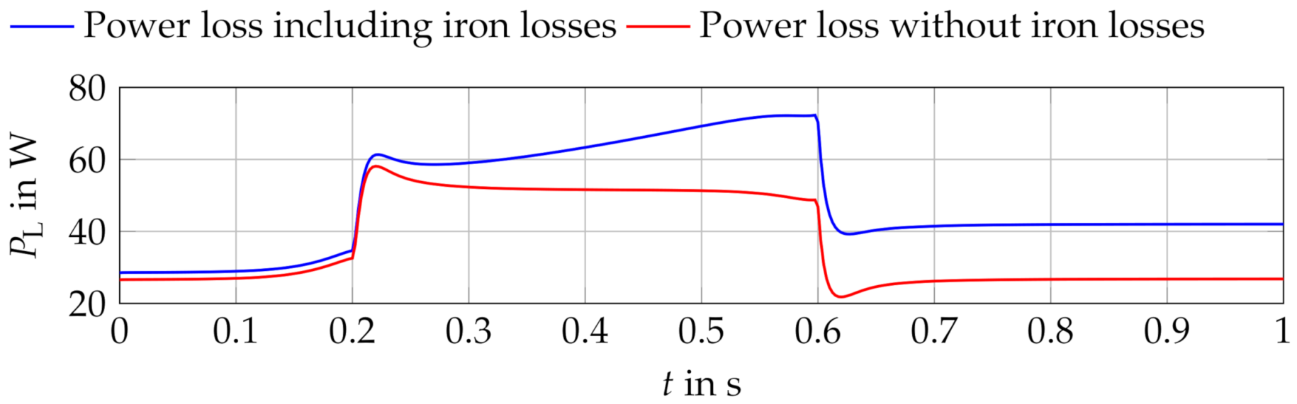
6.2. Influence of Iron Losses
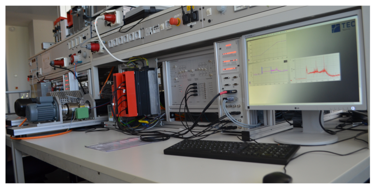
7. Measurements
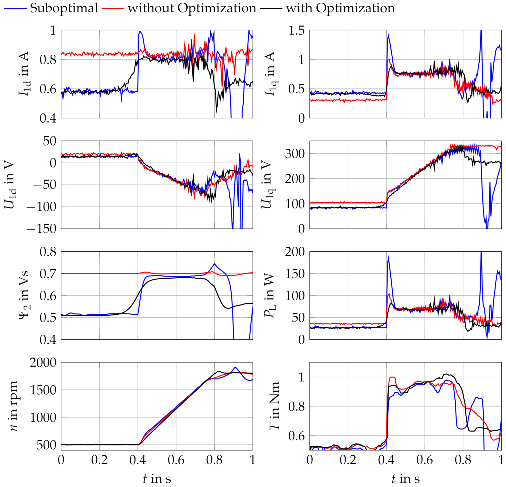
7.1. Optimal Offline Solution
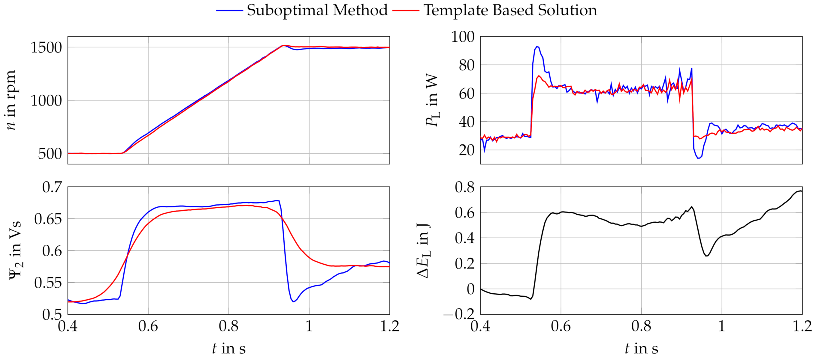
7.2. Template Based Solution
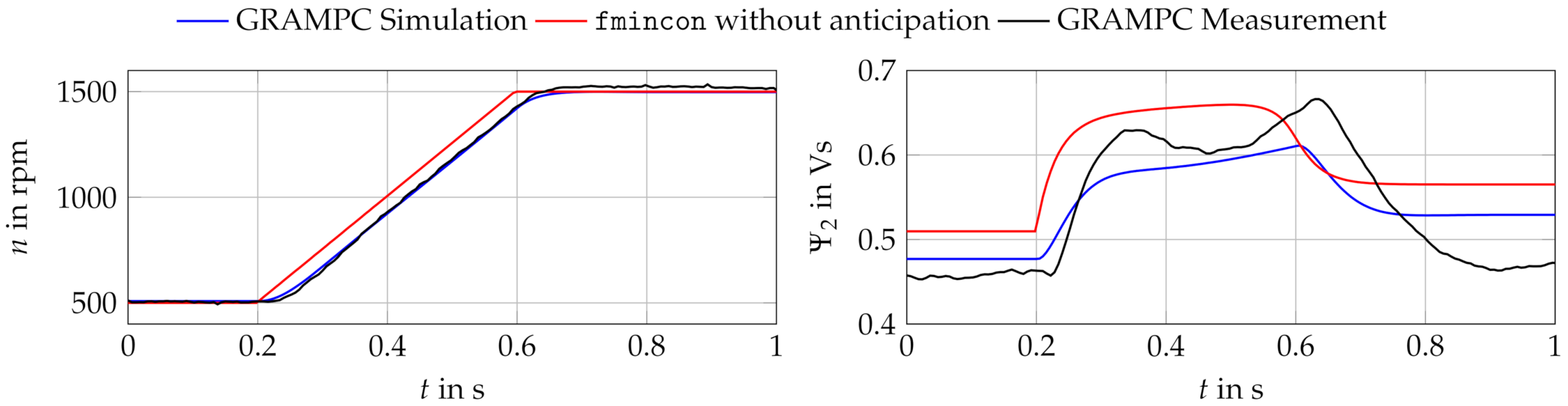
7.3. Model Predictive Solution
8. Application of the Template Based Solution to the WLTP Driving Cycle
9. Conclusions
Author Contributions
Funding
Conflicts of Interest
Nomenclature
| Symbol | Unit | Description |
| 1 | Coefficients of main inductance polynomial | |
| J | Difference in energy lost | |
| J | Energy lost of new approach | |
| J | Energy lost of reference approaches | |
| A | Stator current phasor | |
| A | Stator d-current component | |
| A | Stator optimal d-current component in static operation | |
| A | Reference stator d-current for the current controller | |
| A | Actual stator d-current for the current controller | |
| A | Stator q-current component | |
| A | Maximum stator current phasor length | |
| A | Rotor current phasor | |
| A | Current phasor through main inductance | |
| A | Current phasor through iron resistance | |
| J | 1 | Objective functional |
| 1 | Discretized objective functional | |
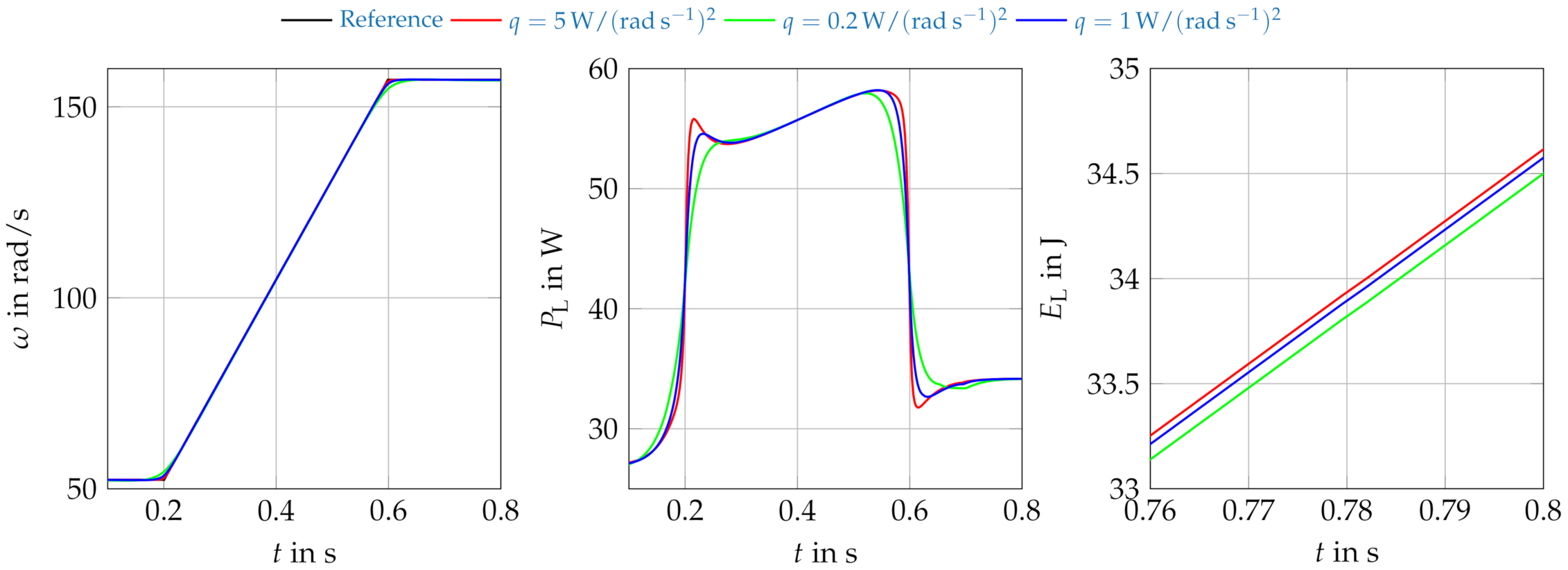
| q | W/(rad s−1)2 | Weightage factor for specifying optimization priorities |
| kgm2 | Moment of inertia of the motor | |
| kgm2 | Moment of inertia of the load | |
| kgm2 | Total moment of inertia of the entire drive train | |
| k | 1 | Sample number counter |
| N | 1 | Total number of samples |
| H | Stray inductance | |
| H | Main inductance | |
| rad/s | Stator angular frequency | |
| rad/s | Slip angular frequency | |
| rad/s | Rotor mechanical angular frequency | |
| rad/s | Rotor mechanical angular frequency reference for the speed controller | |
| rad/s | Actual rotor mechanical angular frequency for the current controller | |
| W | Power loss | |
| Vs | Stator flux linkage d-component | |
| Vs | Stator flux linkage q-component | |
| Vs | Rotor flux linkage phasor | |
| Vs | Rotor flux linkage d-component | |
| Vs | Rotor flux linkage q-component | |
| Vs | Optimal rotor flux linkage | |
| Vs | Optimal rotor flux linkage in static operation | |
| Vs | Rotor flux linkage according to the template | |
| Vs | Rotor flux linkage reference for the flux controller | |
| Vs | Actual rotor flux linkage for the flux controller | |
| Stator copper resistance | ||
| Rotor copper resistance | ||
| Iron resistance | ||
| t | s | Time |
| s | Start time of the optimization interval | |
| s | Anticipative time | |
| s | End time of the optimization interval | |
| s | Rotor time constant | |
| s | Sample time | |
| Nm | Load torque | |
| Nm | Torque produced by the motor | |
| Nm | Reference torque | |
| V | Stator voltage phasor | |
| V | Maximum length of stator voltage phasor | |
| V | Stator voltage d-component | |
| V | Stator voltage q-component | |
| - | Number of pole pairs |
Abbreviations
| fmincon | MATLAB find minimum of constrained nonlinear multivariable function |
| GRAMPC | A gradient-based augmented Lagrangian framework for embedded NMPC |
| WLTP | World Harmonised Light Weight Vehicles Test Procedure |
Appendix A. Motor Parameters

| 370 W | Nm | ||
|---|---|---|---|
| 2 | |||
| 1370 rpm | |||
| −0.669 | 3.606 | ||
| −6.622 | 4.415 | ||
| −0.743 | 0.754 | ||
| 0.42 s | 0.56 s | ||
| 0.62 s | 0.76 s | ||
| 0.9 s | |||
| 0.0013 | 0.5778 | ||
| rad/s 500 rpm | rad/s 1800 rpm | ||
| Nm |
References
- Bailey, G.; Mancheri, N.; van Acker, K. Sustainability of Permanent Rare Earth Magnet Motors in (H)EV Industry. J. Sustain. Metall. 2017, 3, 611–626. [Google Scholar] [CrossRef]
- Rassolkin, A.; Heidari, H.; Kallaste, A.; Vaimann, T.; Acedo, J.P.; Romero-Cadaval, E. Efficiency Map Comparison of Induction and Synchronous Reluctance Motors. In Proceedings of the 2019 26th International Workshop on Electric Drives: Improvement in Efficiency of Electric Drives (IWED), Moscow, Russia, 30 January–2 February 2019; pp. 1–4. [Google Scholar] [CrossRef]
- Kim, S.; Sul, S.K.; Ide, K.; Morimoto, S. Maximum efficiency operation of Synchronous Reluctance Machine using signal injection. In Proceedings of the 2010 International Power Electronics Conference—ECCE ASIA, Sapporo, Japan, 21–24 June 2010; pp. 2000–2004. [Google Scholar] [CrossRef]
- Bazzi, A.M.; Krein, P.T. Review of Methods for Real-Time Loss Minimization in Induction Machines. IEEE Trans. Ind. Appl. 2010, 46, 2319–2328. [Google Scholar] [CrossRef]
- Kioskeridis, I.; Margaris, N. Loss Minimization in Scalar—Controlled Induction Motor Drives with Search Controllers. IEEE Trans. Power Electron. 1996, 11, 213–220. [Google Scholar] [CrossRef]
- Consoli, A.; Scarcella, G.; Scelba, G.; Cacciato, M. Energy Efficient Sensorless Scalar Control for Full Speed Operating Range IM Drives. In Proceedings of the 14th European Conference on Power Electronics and Applications, Birmingham, UK, 30 August–1 September 2011; pp. 1–10. [Google Scholar]
- Uddin, M.N.; Nam, S.W. New Online Loss—Minimization–Based Control of an Induction Motor Drive. IEEE Trans. Power Electron. 2008, 23, 926–933. [Google Scholar] [CrossRef]
- Qu, Z.; Ranta, M.; Hinkkanen, M.; Luomi, J. Loss-Minimizing Flux Level Control of Induction Motor Drives. IEEE Trans. Ind. Appl. 2012, 48, 952–961. [Google Scholar] [CrossRef] [Green Version]
- Windisch, T.; Hofmann, W. A Novel Approach to MTPA Tracking Control of AC Drives in Vehicle Propulsion Systems. IEEE Trans. Veh. Technol. 2018, 67, 9294–9302. [Google Scholar] [CrossRef]
- Chakraborty, C.; Hori, Y. Fast Efficiency Optimization Techniques for the Indirect Vector–Controlled Induction Motor Drives. IEEE Trans. Ind. Appl. 2003, 39, 1070–1076. [Google Scholar] [CrossRef] [Green Version]
- Wang, Y.; Ito, T.; Lorenz, R.D. Loss Manipulation Capabilities of Deadbeat–Direct Torque and Flux Control Induction Machine Drives. IEEE Trans. Ind. Appl. 2015, 51, 4554–4566. [Google Scholar] [CrossRef]
- Lorenz, R.D.; Yang, S.M. Efficiency–Optimized Flux Trajectories for Closed–Cycle Operation of Field-Orientation Induction Machine Drives. IEEE Trans. Ind. Appl. 1992, 28, 574–580. [Google Scholar] [CrossRef]
- Lorenz, R.D.; Yang, S.M. AC Induction Servo Sizing for Motion Control Applications via Loss Minimizing Real–Time Flux Control. IEEE Trans. Ind. Appl. 1992, 28, 589–593. [Google Scholar] [CrossRef]
- Klenke, F.; Hofmann, W. Energy-Efficient Control of Induction Motor Servo Drives With Optimized Motion and Flux Trajectories. In Proceedings of the 14th European Conference on Power Electronics and Applications, Birmingham, UK, 30 August–1 September 2011; pp. 1–7. [Google Scholar]
- Stumper, J.F.; Dötlinger, A.; Kennel, R. Loss Minimization of Induction Machines in Dynamic Operation. IEEE Trans. Energy Convers. 2013, 28, 726–735. [Google Scholar] [CrossRef]
- Borisevich, A.; Schullerus, G. Energy Efficient Control of an Induction Machine Under Torque Step Changes. IEEE Trans. Energy Convers. 2016, 31, 1295–1303. [Google Scholar] [CrossRef]
- Grčar, B.; Hofer, A.; Štumberger, G. Induction Machine Control for a Wide Range of Drive Requirements. Energies 2020, 13, 175. [Google Scholar] [CrossRef] [Green Version]
- Diachenko, G.; Schullerus, G. Simple Dynamic Energy Efficient Field Oriented Control in Induction Motors. In Proceedings of the 18th International Symposium Power Electronics Ee2015, Belgrade, Serbia, 22–24 April 2015; pp. 1–5. [Google Scholar]
- Weis, R.; Gensior, A. A Model-Based Loss-Reduction Scheme for Transient Operation of Induction Machines. EPE 2016, 2016, 1–8. [Google Scholar] [CrossRef]
- Plathottam, S.J.; Salehfar, H. Transient Energy Efficiency Analysis of Field Oriented Induction Machines. IEEE Access 2017, 5, 20545–20556. [Google Scholar] [CrossRef]
- Abdelati, R.; Mimouni, M.F. Optimal control strategy of an induction motor for loss minimization using Pontryaguin principle. Eur. J. Control 2019, 49, 94–106. [Google Scholar] [CrossRef]
- Diachenko, G.G.; Schullerus, G.; Dominic, A.; Aziukovskyi, O.O. Energy-efficient predictive control for field-orientation induction machine drives. Nauk. Visnyk Natsionalnoho Hirnychoho Universytetu 2020, 61–67. [Google Scholar] [CrossRef]
- Hu, Z.; Liu, Q.; Hameyer, K. Loss Minimization of Speed Controlled Induction Machines in Transient States Considering System Constraints. In Proceedings of the 2014 17th International Conference on Electrical Machines and Systems (ICEMS), Hangzhou, China, 22–25 October 2014; pp. 123–129. [Google Scholar] [CrossRef]
- Dominic, A.; Schullerus, G.; Winter, M. Optimal Flux and Current Trajectories for Efficient Operation of Induction Machines. In Proceedings of the 2019 20th International Symposium on Power Electronics (Ee), Novi Sad, Serbia, 23–26 October 2019; pp. 1–6. [Google Scholar] [CrossRef]
- Dominic, A.; Schullerus, G.; Winter, M. Anticipative Flux Trajectories for Dynamic Energy Efficient Operation of Induction Machines. In Proceedings of the 2020 IEEE Transportation Electrification Conference & Expo (ITEC), Chicago, IL, USA, 24–26 June 2020; pp. 1038–1043. [Google Scholar] [CrossRef]
- Dominic, A.; Schullerus, G.; Winter, M. Rotor Flux Templates for Energy Efficient Dynamic Operation of Induction Machines. In Proceedings of the 2020 International Conference on Electrical Machines (ICEM), Gothenburg, Sweden, 23–26 August 2020; pp. 312–318. [Google Scholar] [CrossRef]
- Englert, T.; Völz, A.; Mesmer, F.; Rhein, S.; Graichen, K. A software framework for embedded nonlinear model predictive control using a gradient-based augmented Lagrangian approach (GRAMPC). Optim. Eng. 2019, 20, 769–809. [Google Scholar] [CrossRef] [Green Version]
- Quang, N.P.; Dittrich, J.A. Vector Control of Three-Phase AC Machines: System Development in the Practice; Power Systems; Springer: Berlin/Heidelberg, Germany, 2008. [Google Scholar]
- Pucci, M. State-Space Space-Vector Model of the Induction Motor Including Magnetic Saturation and Iron Losses. IEEE Trans. Ind. Appl. 2019, 55, 3453–3468. [Google Scholar] [CrossRef]
- United Nations. Global Registry, Created on 18 November 2004, Pursuant to Article 6 of the Agreement Concerning the Establishing of Global Technical Regulations for Wheeled Vehicles, Equipment and Parts Which Can Be Fitted and/or Be Used on Wheeled Vehicles (ECE/TRANS/132 and Corr.1) Done at Geneva on 25 June 1998: Addendum 15: Global Technical Regulation No. 15, Worldwide Harmonized Light Vehicles Test Procedure: Established in the Global Registry on 12 March 2014; United Nations: New York, NY, USA, 2014. [Google Scholar]


Publisher’s Note: MDPI stays neutral with regard to jurisdictional claims in published maps and institutional affiliations. |
© 2021 by the authors. Licensee MDPI, Basel, Switzerland. This article is an open access article distributed under the terms and conditions of the Creative Commons Attribution (CC BY) license (http://creativecommons.org/licenses/by/4.0/).
Share and Cite
Dominic, A.; Schullerus, G.; Winter, M. Dynamic Energy Efficient Control of Induction Machines Using Anticipative Flux Templates. Appl. Sci. 2021, 11, 2878. https://doi.org/10.3390/app11062878
Dominic A, Schullerus G, Winter M. Dynamic Energy Efficient Control of Induction Machines Using Anticipative Flux Templates. Applied Sciences. 2021; 11(6):2878. https://doi.org/10.3390/app11062878
Chicago/Turabian StyleDominic, Antony, Gernot Schullerus, and Martin Winter. 2021. "Dynamic Energy Efficient Control of Induction Machines Using Anticipative Flux Templates" Applied Sciences 11, no. 6: 2878. https://doi.org/10.3390/app11062878