Synthetic Study of Boulder Detection Using Multi-Configuration Combination of Cross-Hole ERT and Its Field Application in Xiamen Metro, China

Abstract

With the fast development of urban rail transportation, shield construction has been widely used in tunnel construction in China. It is very important to detect the random distribution of boulders, which may cause geological problems. Cross-hole electrical resistivity tomography (ERT) has the advantage of precise detection, but it has not been systematically studied in solitary rock detection. Therefore, we set up several numerical models and proposed weighted inversion, to improve the capacity for detecting boulders. Subsequently, the method was applied to the Xiamen Metro Line 1, where it was highly likely to encounter boulders. All the test boreholes revealed the presence of boulders, and their location and size were consistent with the geophysics results. This study demonstrated the suitability of weighted inversion based on a multi-configuration combination of cross-hole ERT for the detection of boulders. This case study provides new engineering perspectives on how to detect boulders.

1. Introduction

In recent years, subways have been extensively constructed because of the limitations and increasing pressure from the demand on land resources and the growing urban population. Meanwhile, shield tunneling has been more and more widely used in metro tunnel construction, and the excavation depth of shield tunnels is becoming deeper than before. Deep boulders have become one of the problems threatening subway tunnel construction. However, the spacing between drilling holes in metro engineering is usually 40–50 m [1]. Such a distance leads to a low probability of discovering boulders. As a result, the detection of boulders is tremendously challenging.

In the last few decades, geophysical prospecting techniques [2,3,4] and inversion methods [5] have made great progress, and some have been used in engineering, proving their validity [6,7,8,9,10,11,12,13,14,15]. At the same time, some geophysical exploration methods have been applied to identify boulders, including ground-penetrating radar [12] and microtremor surveying [1]. However, the resolution of surface prospecting methods is limited, and the low signal-to-noise ratio creates the possibility of increased artifacts [1,16]. As it stands, the underground surroundings of subway tunnel construction projects are usually complicated, and the occurrence and condition of boulders within the strata are unpredictable. Therefore, methods for improving the accuracy of boulder detection need to be developed.

Cheng et al. [17] applied cross-hole seismic tomography analysis to detect boulders, and Li et al. [2] analyzed the effect of cross-hole ERT in the detection of boulders using model testing. By comparing with surface prospecting methods, cross-hole methods were found to be effective for improving the resolution at depth. The capability of cross-hole ERT exceeds the performance limits of surface electrical surveying, because it extends the detection range [18]. Liu et al. [19] used an optimized refraction tomography method to accurately determine a tunnel’s geology. Nie et al. [20,21] used the ERT method to detect underground abnormal bodies in physical models and practical engineering. In previous studies, cross-hole ERT was used for many aspects. For instance, cross-hole ERT was applied to hydrogeological and fluid/gas plume migration studies, allowing better monitoring of the variations of those processes and the characterization of subsurface structures [22]. These studies have shown the prospects of success with this technique in our study area. Hence, it is natural to choose cross-hole ERT as one of the geophysical methods for detecting boulders. Previous studies on cross-hole ERT found that every configuration has its own advantages and disadvantages [18,23]. Therefore, we proposed multi-configuration combinations of cross-hole ERT.

The study herein focused on the application of the cross-hole ERT method in detecting boulders. First, we put forward an weighted inversion model, based on a multi-configuration combination of cross-hole ERT. We set up several numerical examples, to verify the correctness of the method. Then, the method was applied to practical projects. A multi-configuration combination of cross-hole ERT was used to collect data, followed by data processing that used the weighted inversion to obtain four profiles. Finally, the study evaluated the effectiveness of this method, by analyzing the results of field tests.

2. Methods and Simulation of Boulder Detection Using Cross-Hole ERT

2.1. Different Configurations and Sensitivity Analysis

This study used three configurations, including a dipole–dipole array, bipole–bipole array, and pole–tripole array, which were defined as follows (Figure 1): the current and potential poles in different boreholes for the dipole–dipole array (Figure 1a); one current pole and one potential pole in the same borehole for the bipole–bipole array (Figure 1b); and a first current electrode in one borehole and three other electrodes in the other borehole for the pole–tripole array (Figure 1c).

The sensitivity of the used arrays is shown, as follows: From Figure 2, we can see that these three configurations have the highest sensitivity at the electrode point. The sensitivity distribution shows that three configurations have a good horizontal resolution and poor vertical resolution.

2.2. Multi-Configuration Combination, Based on Weighting Factor

According to the analysis of Leontarakis and Apostolopoulos [23], the signal of the bipole–bipole array is stronger and sensitive, even for a relatively small target. However, when the environment becomes more complex, the resolution of the array can be reduced. While, the resolution of the pole–tripole array is excellent, even in a complex environment, but the results of some studies featured many artifacts. Furthermore, Zhou and Greenhalgh [18] found that a disadvantage of the dipole–dipole array is that the potential difference measured by this array is smaller and more easily masked by noise, which in turn decreases the resolution.

Considering the cumulative factors of these three measurement techniques, the electrical resistivity measurement chosen was a multi-configuration combination, consisting of the three cross-hole configurations as described above, including a dipole–dipole array, bipole–bipole array, and pole–tripole array. The electrode spacing of the dipole–dipole array varied within the interval, which was guaranteed to collect more overall data. Moreover, the spacing of the electrodes of the bipole–bipole array was 2 m, while for the pole–tripole array it was 1–3 m. The test applied this multi-configuration combination, featuring the superposition of all three cross-hole configurations, to perform the numerical calculations.

At the same time, in order to equalize the participation of the data of each configuration, a particular weighting factor was introduced to improve distinguishability [24]. The magnitude of the weighting factor was based on the Jacobian matrices, $J_A$, $J_B$ and $J_C$, of the three configurations. Following previous research, in this study, the sum of the ratios between $J_j^A$ and $J_j^B$ gives the magnitude of the weighting factor, which is defined as Equation (1):

$$J_j^A=\frac{{{\displaystyle \sum }}_{i=1}^{N_A}\left|J_{ij}^A\right|}{N_A}, J_j^B=\frac{{{\displaystyle \sum }}_{i=1}^{N_B}\left|J_{ij}^B\right|}{N_B}, J_j^C=\frac{{{\displaystyle \sum }}_{i=1}^{N_C}\left|J_{ij}^C\right|}{N_C}$$

(1)

$$b={{\displaystyle \sum }}_{j=1}^M\frac{J_j^A}{J_j^B}(j = 1,2\dots M), c={{\displaystyle \sum }}_{j=1}^M\frac{J_j^A}{J_j^C} (j = 1,2\dots M)$$

(2)

$$J_B=J_{B0}*c, J_C=J_{C0}*c$$

(3)

where $A$ is the bipole–bipole array, $B$ is the pole–tripole array, and $C$ is the dipole–dipole array. By comparison of the numerical simulation tests, the results of selecting the bipole–bipole array as $A$ were more accurate. Thus, $b$ is the weighting factor of the pole–tripole array, and c is the weighting factor of the dipole–dipole array. Meanwhile, the weighting factor for the bipole–bipole array is 1. In this process, $J_j^A$ are the average values of the absolute value of $J_{ij}^A$, which is every element in one column of the bipole–bipole array; while $J_{ij}^B$ are the average values of the absolute value of $J_{ij}^B$, which is every element in one column of the dipole–dipole array or pole–tripole array. Finally, the Jacobian matrices were multiplied by the weighting factor, to balance the contribution of each of the arrays, as in Equation (2).

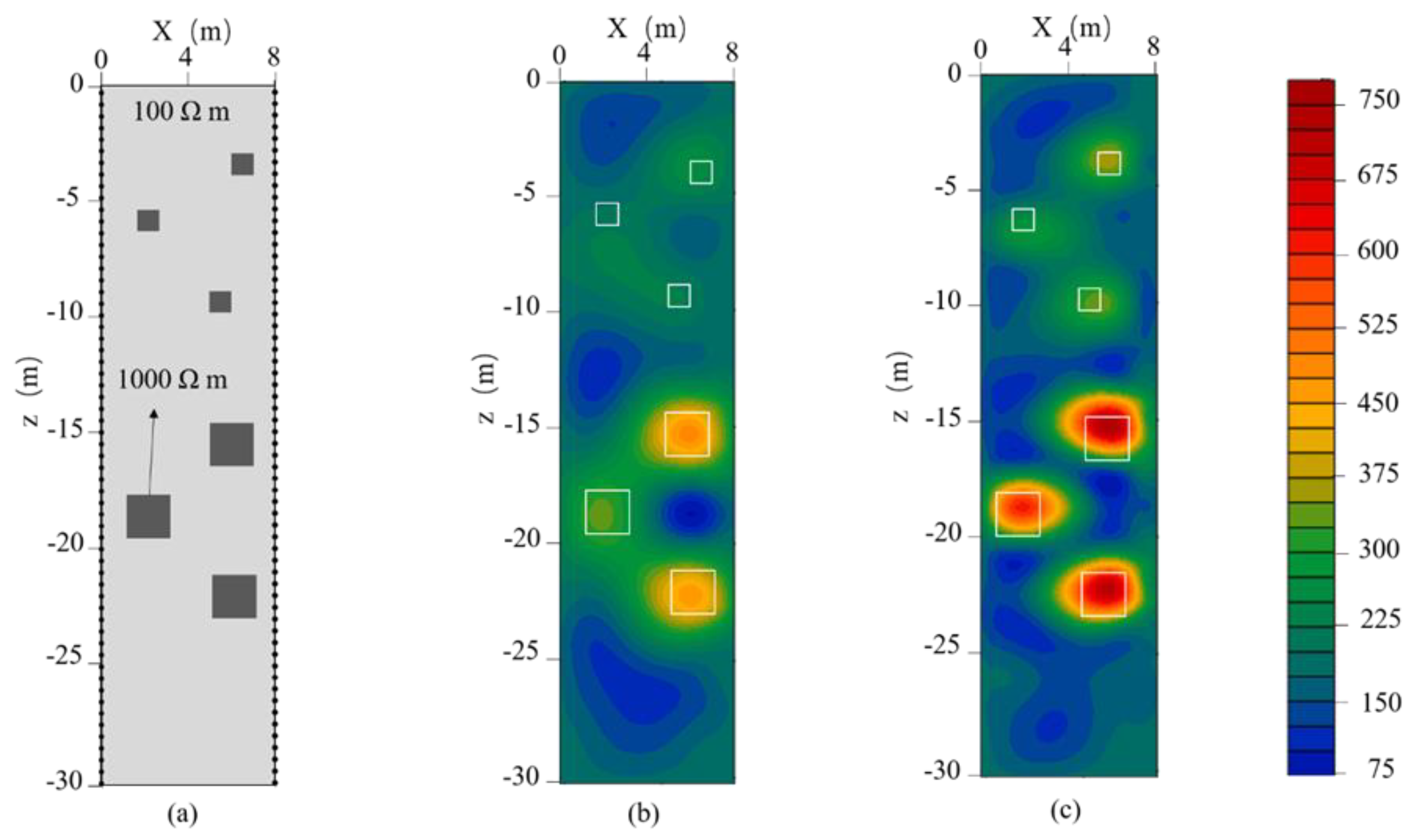
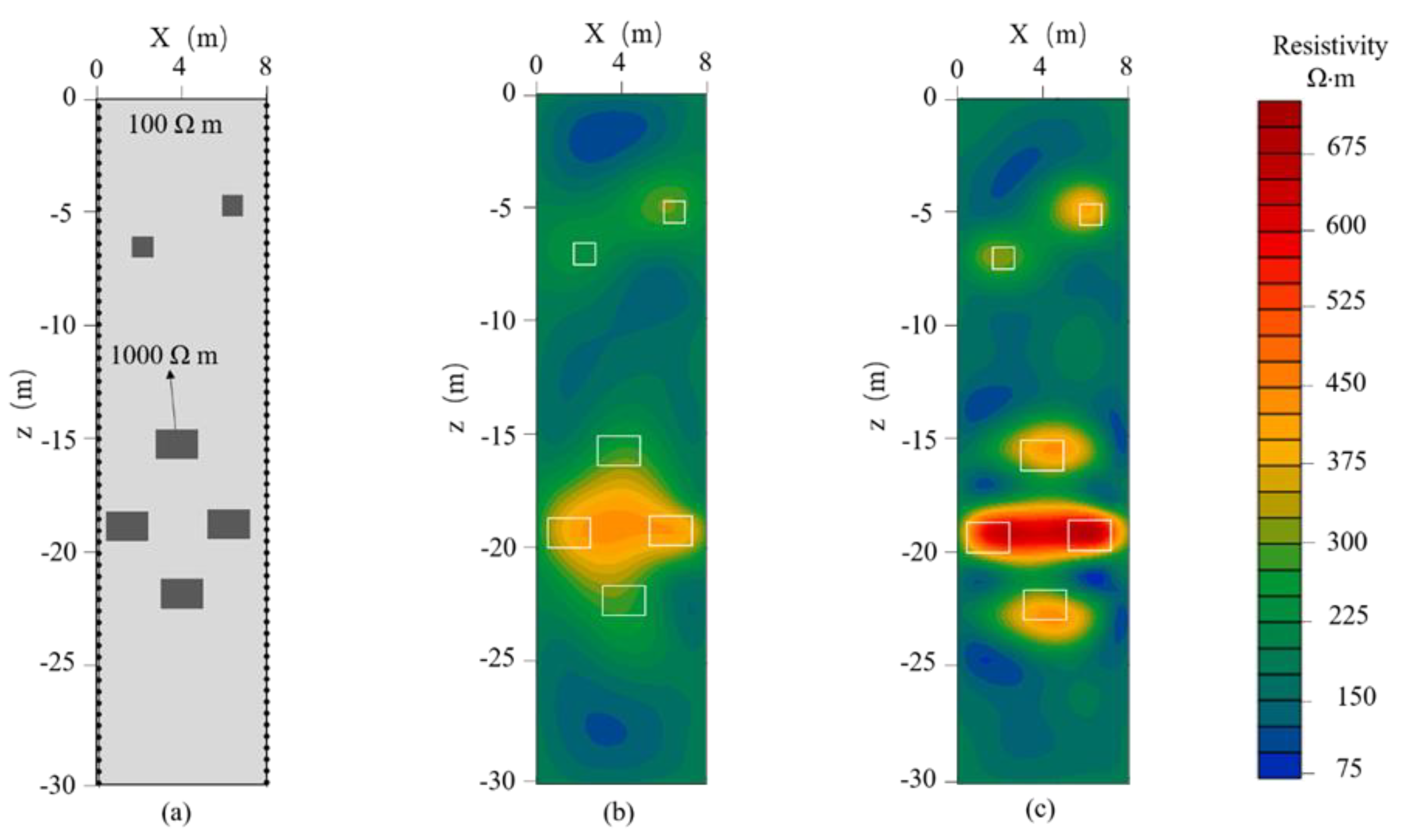
2.3. Numerical Examples

This algorithm was applied to a synthetic resistivity model, which was designed to obtain knowledge about the value of the weighting factor for the detection of boulders. The model included two boreholes, 8 m apart and 30 m in depth, located in a 100 Ω·m homogeneous half-space. One cable with 60 electrodes was installed in each borehole, and the electrode spacing was 0.5 m. Considering that boulders are characterized by high resistivity, the model was set up for targets of 1000 Ω·m within the half-space.

Following this, the inversion results showing whether the weighting factor should be added or not were contrasted to show whether the distinguishability had been improved. According to actual engineering situations, the side length of abnormal bodies buried below 10 m is usually no more than 1 m, while the side length of abnormal bodies buried above 15 m is usually about 2 m. Based on this, we design three numerical simulation examples. In each figure that follows, the geoelectrical models were obtained by the multi-configuration combination and weighted inversion of a multi-configuration combination.

We placed four targets in the first example. Two square targets with a side length of 1 m were placed at 5 m, and the other two square targets with a side length of 2 m were placed at 16 m and 19 m. The results, which include the four targets, is presented in Figure 3. Comparing Figure 3b,c, the deepest target can be identified by increasing the weight factor, and the boundary of the deep boulders is clear. Furthermore, we can see that the resistivity inversion of the shallow anomalous body was about 280 Ω·m and that of the deep anomalous body was more than 500 Ω·m. Figure 4 presents the geoelectrical models with three targets with a side length of 1 m set at 3 m, 6 m, and 9 m, and three targets with a side length of 2 m are set at 15 m, 18 m, and 21 m. Comparing the result with no weighting factor (Figure 4b) and the result when using the weighting factor (Figure 4c) showed that the resolution was improved. When no weighting factor was added, the target bodies near-surface could not be clearly distinguished from the background and the result could not identify the boundaries of the three deep targets. Contrastingly, the model using the weighted inversion (Figure 4c) showed the approximate position of each of the six targets and identified the boundary of the three deep targets’ bodies. In addition, we found that the resistivity of the deeper anomaly was higher than that of the shallow anomaly in the simulation result.

Similarly, the resistivity model, including six targets, with two scattered bodies near the surface and the other four deeper agminated bodies, is shown in Figure 5a. Two targets with a side length of 1 m were set at 3 m and 6 m, and four targets with a side length of 2 m were set at 15 m, 17 m, and 22 m. Only a deep body and a bar object can be seen in the result with no weighting factor (Figure 5b). Moreover, considering the volume effect of the electrical exploration and sensitivity distribution, the cross-hole ERT has good vertical resolution and weak horizontal resolution, and the resolution of the multiple targets at the same horizontal position is limited (Figure 5c).

From the comparison of the above three groups, it is apparent that the weighted inversion geoelectrical model was significantly better than the model produced by the inversion of the multi-configuration combination with no weighting factor. In addition, the inversion results show that the resistivity of the deep target was always higher than that of the shallow target. In other words, deep anomalies had a better resolution than shallow anomalies.

3. Field Case

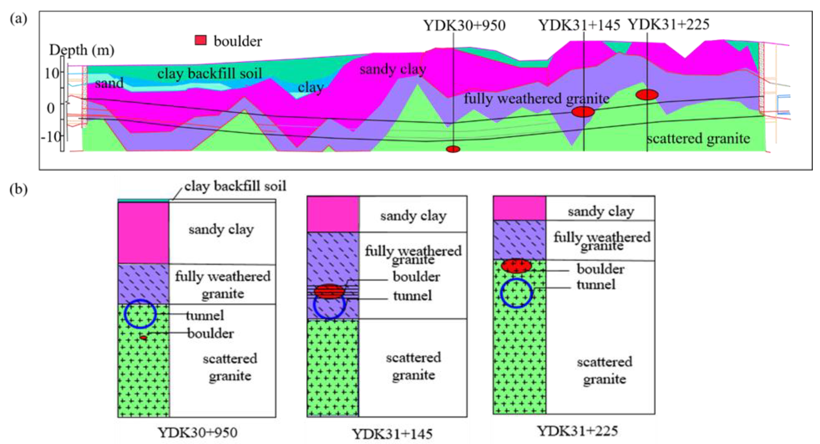
3.1. Geological Background

Xiamen Metro Line 1, which forms a cross-sea passage between Xiamen Island and Jimei District, is located in Xiamen, Fujian Province, China. The research selected a section between the locations of Station Tianshui and Station Xiamen north (Figure 6). There were many limiting factors between the two stations, such as many houses above the tunnel and a narrow and disordered road. The longitudinal section of the interval is a v-shaped slope. The depth range of the tunnel is 10.8 to 21 m. The geology of this section mainly passes through residual sandy cohesive soil, completely weathered granite, and granular strongly weathered granite. The overlying strata of this section are clay, clay quality fill, completely weathered granite, and granular strongly weathered granite, while the underlying strata are granite and diabase. The section mainly passes through the eluvium, and the boulders are relatively developed (Figure 7a). From the geological survey data, the studied zone mainly traverses eluvial strata, which is well distributed with boulders of a relatively small size and volume. It can be seen from the coring results (Figure 7b) that boulders appeared frequently and their positions were random, which indicates that the detection of boulders in this strata interval is of high difficulty and challenging. It is of practical engineering value to use geophysical methods to detect the existence of boulders under limited conditions.

3.2. Layout of the Cross-Hole ERT Survey Lines

Considering that the boulders at the edge of the shield machine have a great impact on the cutterhead, the study was designed to detect the contour of the tunnel. Moreover, due to the limitation of the surface environment and the close distance between the left and right lines of the tunnel, only the space between the tunnels was surveyed in the detection process. Therefore, apparent resistivity measurements were made using the four survey lines arranged on the surface, using five existing boreholes, as shown in Figure 8. The lengths of the survey lines were 11.55, 9.5, 9.8, and 10.5 m, respectively, measuring from northeast to southwest. We used nonpolarized electrodes, and the electrode spacing on the cable was 1 m. To ensure the electrical contact between soil and electrodes, we poured water into the borehole to couple them. In practice, it was necessary to verify whether the results of the geophysical prospecting were precise. The results of the weighted inversion of the multi-configuration combination were compared with the actual field measuring results using the test boreholes. The locations of four test boreholes (YZK1–YZK4; Figure 8) were delineated using the results of geophysical prospecting.

3.3. Results and Discussion

In this section, four profiles and four coring results of test boreholes are described, to indicate the position of boulders in the studied area. Each profile was obtained by weighted inversion of the multi-configuration combination, as shown in Figure 9. In this process, the smoothness-constrained least-squares inversion method was applied to invert resistivity data and the number of iterations of inversion was six. The coring result of the test boreholes is shown in Figure 9, in comparison with the weighted inversion results of the field data.

The four profiles showed high resistivity values in areas corresponding to the boulders. Figure 9a shows three high-resistivity bodies between ZK4 and ZK5 at different positions.

In YZK1 (Figure 9a), cross-hole ERT revealed three boulders, located at a depth of 5–10 m, depth of 18–22 m, and depth of 27–30 m. Correspondingly, the borehole revealed an abnormal body located at 23–27 m.

The profile for the site between ZK4 and ZK1 is shown in Figure 9b. Cross-hole ERT also revealed three boulders, which were located at a depth of 5–10 m, depth of 18–22 m, and depth of 27–30 m. Correspondingly, the borehole revealed an abnormal body located at 25–28 m.

The profiles in Figure 9c were acquired between ZK3 and ZK1, showing three high resistivity bodies. The test borehole revealed two boulders at 21–23 m and 27–31 m. It is noted that the results obtained by geophysical prospecting found one more high resistivity body than the coring results of YZK3.

Figure 9d shows very similar features to Figure 9c, for the site between ZK2 and ZK1. Three high resistivity bodies occurred at 12–15, 17–21, and 23–27 m. The results of the test borehole presented in Figure 9d included two boulders. One was at 20–23 m and another was at 23–27 m. Compared with three the bodies in the profile between ZK2 and ZK1 (Figure 9d), there existed one different body, at 12–15 m.

From the perspective of numerical simulation, the new cross-hole ERT method has good vertical resolution and weak horizontal resolution, but it may be difficult to distinguish boulders of the same horizontal position and size, independently. Moreover, from the numerical simulation and engineering measurement, when setting a reasonable borehole-depth/borehole-spacing ratio (>1.5) and borehole spacing and electrode spacing, boulders with a size of 0.5 m~2 m can be distinguished.

Based on the analysis herein, the results of the geophysical prospecting showed a high degree of similarity with the results of the test boreholes. Moreover, the ERT results show more boulder anomalies. The cross-hole ERT results showed more high resistivity bodies, and they were some distance from the test boreholes. These could have been boulders that were outside the test boreholes. Results using the weighted inverted geoelectrical model were reasonable and agreed with the results validated by the boreholes. This study demonstrates that the use of weighted inversion of a multi-configuration combination in the investigation of boulder detection is effective. Therefore, we recommend the use of weighted inversion of a multi-configuration combination as a higher resolution approach to detection. However, in the application of this method, a few disadvantages were found. For instance, the boundaries of bodies were unclear. Therefore, further basic research is required, to solve problems such as the multi-scale inversion [25] and L1 (blocky) inversion.

4. Conclusions

The ability to detect and characterize shallow boulders below the surface can enable optimization of the construction plan of tunnels in advance, to reduce and avoid hazards. We put forward a multi-configuration combination of cross-hole ERT based on weighting, to improve the detection capability. Then, the method was applied to an engineering case, and the effectiveness of the method was proven using test boreholes.

Moreover, in order to ensure the safety of construction workers and of the shield machine while operating in a tunnel, we offer several suggestions based on this study. First, it is advised that when conducting boulder detection using the cross-hole ERT method, the quality of casing drilling should be strictly controlled. Second, it is essential to ensure that the depth and spacing of boreholes meet the requirements. The reason for this is that the spacing of the holes should not exceed approximately 0.75 times the hole array length, to guarantee achieving a rational image resolution [21,26]. Finally, boulders that have been detected should be disposed of in a timely manner.

References

1. Li, B.; Wu, L.; Xu, C.; Zuo, Q.; Wu, S.; Zhu, B. The Detection of the Boulders in Metro Tunneling in Granite Strata Using a Shield Tunneling Method and a New Method of Coping with Boulders. Geotech. Geol. Eng. 2016, 34, 1155–1169. [Google Scholar] [CrossRef]
2. Li, S.; Liu, B.; Xu, X.; Nie, L.; Liu, Z.; Song, J.; Sun, H.; Chen, L.; Fan, K. An overview of ahead geological prospecting in tunneling. Tunn. Undergr. Space Technol. 2017, 63, 69–94. [Google Scholar] [CrossRef]
3. Li, S.; Liu, B.; Ren, Y.; Chen, Y.; Yang, S.; Wang, Y.; Jiang, P. Deep-Learning Inversion of Seismic Data. IEEE Trans. Geosci. Remote. Sens. 2019, 58, 2135–2149. [Google Scholar] [CrossRef] [Green Version]
4. Liu, B.; Guo, Q.; Li, S.; Liu, B.; Ren, Y.; Pang, Y.; Guo, X.; Liu, L.; Jiang, P. Deep Learning Inversion of Electrical Resistivity Data. IEEE Trans. Geosci. Remote. Sens. 2020, 58, 5715–5728. [Google Scholar] [CrossRef] [Green Version]
5. Liu, B.; Pang, Y.; Mao, D.; Wang, J.; Liu, Z.; Wang, N.; Liu, S.; Zhang, X. A rapid four-dimensional resistivity data inversion method using temporal segmentation. Geophys. J. Int. 2020, 221, 586–602. [Google Scholar] [CrossRef]
6. Benyassine, E.M.; Lachhab, A.; Dekayir, A.; Parisot, J.C.; Rouai, M. An Application of Electrical Resistivity Tomography to Investigate Heavy Metals Pathways. J. Environ. Eng. Geophys. 2017, 22, 315–324. [Google Scholar] [CrossRef]
7. Guo, Q.; Pang, Y.; Liu, R.; Liu, B.; Liu, Z. Integrated Investigation for Geological Detection and Grouting Assessment: A Case Study in Qingdao Subway Tunnel, China. J. Environ. Eng. Geophys. 2019, 24, 629–639. [Google Scholar] [CrossRef]
8. Li, S.; Xu, S.; Nie, L.; Liu, B.; Liu, R.; Zhang, Q.; Zhao, Y.; Liu, Q.; Wang, H.; Liu, H.; et al. Assessment of electrical resistivity imaging for pre-tunneling geological characterization—A case study of the Qingdao R3 metro line tunnel. J. Appl. Geophys. 2018, 153, 38–46. [Google Scholar] [CrossRef]
9. Lin, C.-P.; Hung, Y.-C.; Wu, P.-L.; Yu, Z.-H. Performance of 2-D ERT in Investigation of Abnormal Seepage: A Case Study at the Hsin-Shan Earth Dam in Taiwan. J. Environ. Eng. Geophys. 2014, 19, 101–112. [Google Scholar] [CrossRef]
10. Bin, L.; Zhengyu, L.; Shucai, L.; Lichao, N.; Maoxin, S.; Huaifeng, S.; Kerui, F.; Xinxin, Z.; Yonghao, P. Comprehensive surface geophysical investigation of karst caves ahead of the tunnel face: A case study in the Xiaoheyan section of the water supply project from Songhua River, Jilin, China. J. Appl. Geophys. 2017, 144, 37–49. [Google Scholar] [CrossRef]
11. Majzoub, A.F.; Stafford, K.W.; Brown, W.A.; Ehrhart, J.T. Characterization and Delineation of Gypsum Karst Geohazards Using 2D Electrical Resistivity Tomography in Culberson County, Texas, USA. J. Environ. Eng. Geophys. 2017, 22, 411–420. [Google Scholar] [CrossRef]
12. Martínez-Pagán, P.; Cano, F.; Aracil, E.; Arocena, J.M. Electrical Resistivity Imaging Revealed the Spatial Properties of Mine Tailing Ponds in the Sierra Minera of Southeast Spain. J. Environ. Eng. Geophys. 2009, 14, 63–76. [Google Scholar] [CrossRef]
13. Nie, L.; Ma, Z.; Wang, C.; Liu, R.; Liu, Z.; Zhou, W.; Li, J.; Ju, S. Integrated ERT, Seismic, and Electrical Resistivity Imaging for Geological Prospecting on Metro Line R3 in Qingdao, China. J. Environ. Eng. Geophys. 2019, 24, 537–547. [Google Scholar] [CrossRef]
14. Wilkinson, P.B.; Chambers, J.; Meldrum, P.I.; Ogilvy, R.D.; Caunt, S. Optimization of Array Configurations and Panel Combinations for the Detection and Imaging of Abandoned Mineshafts using 3D Cross-Hole Electrical Resistivity Tomography. J. Environ. Eng. Geophys. 2006, 11, 213–221. [Google Scholar] [CrossRef] [Green Version]
15. Li, L.; Tan AE, C.; Jhamb, K.; Rambabu, K. Buried object characterization using ultra-wideband ground penetrating radar. IEEE Trans. Microw. Theory Tech. 2012, 60, 2654–2664. [Google Scholar] [CrossRef]
16. Perri, M.T.; Cassiani, G.; Gervasio, I.; Deiana, R.; Binley, A. A saline tracer test monitored via both surface and cross-borehole electrical resistivity tomography: Comparison of time-lapse results. J. Appl. Geophys. 2012, 79, 6–16. [Google Scholar] [CrossRef]
17. Cheng, F.; Liu, J.; Wang, J.; Zong, Y.; Yu, M. Multi-hole seismic modeling in 3-D space and cross-hole seismic tomography analysis for boulder detection. J. Appl. Geophys. 2016, 134, 246–252. [Google Scholar] [CrossRef]
18. Bing, Z.; Greenhalgh, S. Cross-hole resistivity tomography using different electrode configurations. Geophys. Prospect. 2000, 48, 887–912. [Google Scholar] [CrossRef]
19. Liu, S.; Jia, Z.; Zhu, Y.; Zhao, X.; Cheng, S. Optimized Refraction Travel Time Tomography. Appl. Sci. 2019, 9, 5439. [Google Scholar] [CrossRef] [Green Version]
20. Nie, L.; Shen, J.; Zhou, P.; Liu, Z.; Pang, Y.; Zhou, W.; Chen, A. Cross-hole ERT Configuration Assessment for Boulder Detection: A Full-scale Physical Model Test. J. Environ. Eng. Geophys. 2020, 25, 569–579. [Google Scholar] [CrossRef]
21. Bellmunt, F.; Marcuello, A.; Ledo, J.; Queralt, P. Capability of cross-hole electrical configurations for monitoring rapid plume migration experiments. J. Appl. Geophys. 2016, 124, 73–82. [Google Scholar] [CrossRef]
22. Leontarakis, K.; Apostolopoulos, G.V. Laboratory study of the cross-hole resistivity tomography: The Model Stacking (MOST) Technique. J. Appl. Geophys. 2012, 80, 67–82. [Google Scholar] [CrossRef]
23. Athanasiou, E.; Tsourlos, P.; Papazachos, C.; Tsokas, G. Combined weighted inversion of electrical resistivity data arising from different array types. J. Appl. Geophys. 2006, 62, 124–140. [Google Scholar] [CrossRef]
24. Pang, Y.; Nie, L.; Liu, B.; Liu, Z.; Wang, N. Multiscale resistivity inversion based on convolutional wavelet transform. Geophys. J. Int. 2020, 223, 132–143. [Google Scholar] [CrossRef]
25. Labrecque, D.J.; Ramirez, A.L.; Daily, W.D.; Binley, A.; Schima, S.A. ERT monitoring of environmental remediation processes. Meas. Sci. Technol. 1996, 7, 375–383. [Google Scholar] [CrossRef]
26. Loke, M.H.; Chambers, J.E.; Rucker, D.F.; Kuras, O.; Wilkinson, P.B. Recent developments in the direct-current geoelectrical imaging method. J. Appl. Geophys. 2013, 95, 135–156. [Google Scholar] [CrossRef]
Figure 1. Cross-hole ERT configurations; A and B represent the current electrodes and, M and N represent the potential electrodes: (a) dipole–dipole array (AB = n, n = 3, 5; MN = m, m = 2, 3, 4, 5, 6); (b) bipole–bipole array (AM = n, n = 2, 3, 4, 5, 6; BN = m, m = 2, 3, 4, 5, 6); and (c) pole–tripole array (BM = n, n = 2, 3, 4, 5, 6; BN = m, m = 2, 3, 4, 5, 6).
Applsci 11 11860 g001
Figure 2. Sensitivity distribution of cross-hole ERT configurations: A and B represent the current electrodes, and M and N represent the potential electrodes: (a) dipole-dipole array; (b) bipole-bipole array; and (c) pole-tripole array.
Applsci 11 11860 g002
Figure 3. Simulation result with four targets: (a) model (background: 100 Ω·m; simulated boulder (high resistivity anomaly): 1000 Ω·m); (b) the results of the multi-configuration combination; and (c) the results of weighted inversion of the multi-configuration combination.
Applsci 11 11860 g003
Figure 4. Simulation result with six targets, which included three near the surface and others deeper: (a) model (background: 100 Ω·m; simulated boulder (high resistivity anomaly): 1000 Ω·m); (b) the results of the multi-configuration combination; and (c) the results of the weighted inversion of the multi-configuration combination.
Applsci 11 11860 g004
Figure 5. Simulation result, including six targets, with two near the surface and the other four deeper: (a) model (background: 100 Ω·m; simulated boulder (high resistivity anomaly): 1000 Ω·m); (b) the results of the multi-configuration combination; and (c) the results of the weighted inversion of the multi-configuration combination.
Applsci 11 11860 g005
Figure 6. Geographical map of the Xiamen rail transit line 1 (between Station Tianshui to Station Xiamen North): (a) the location of Xiamen Metro on the map of China; (b) specific location of Xiamen Metro Line 1; (c) field test.
Applsci 11 11860 g006
Figure 7. Geological sketch map of the area of investigations: (a) stratum profile; (b) the results of borehole data.
Applsci 11 11860 g007
Figure 8. Arrangement of survey lines, boreholes and test boreholes.
Applsci 11 11860 g008
Figure 9. Comparison between the weighted inversion results of field data and the results of the test boreholes: (a) cross-hole electrical resistivity profile of the site between ZK4 to ZK5 and the results of ZK1; (b) cross-hole electrical resistivity profile of the site between ZK4 to ZK1 and the results of ZK2; (c) cross-hole electrical resistivity profile of the site between ZK3 to ZK1 and the results of ZK3; and (d) cross-hole electrical resistivity profile of the site between ZK2 to ZK1 and the results of ZK4.
Applsci 11 11860 g009
Publisher’s Note: MDPI stays neutral with regard to jurisdictional claims in published maps and institutional affiliations.