
Steel Surface Defect Classification Based on Small Sample Learning


Abstract
:1. Introduction
2. Principles and Methodology
2.1. Feature Extraction Network (FEN)
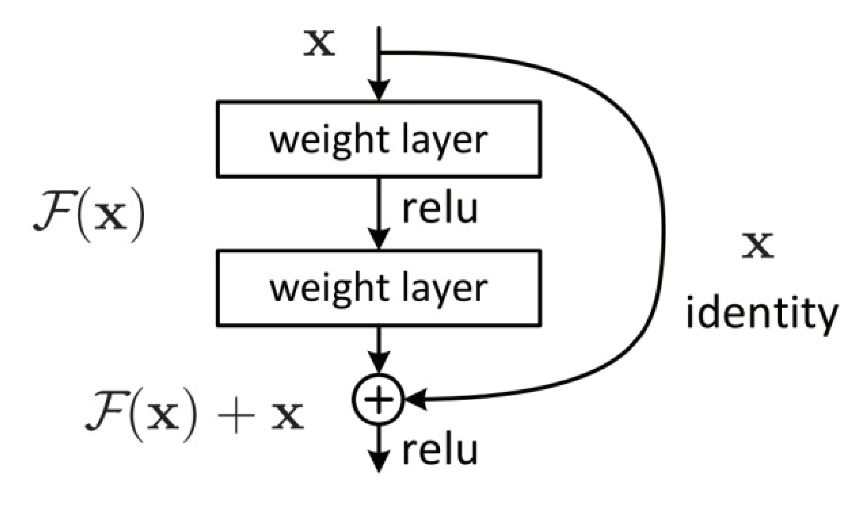
2.1.1. Residual Net
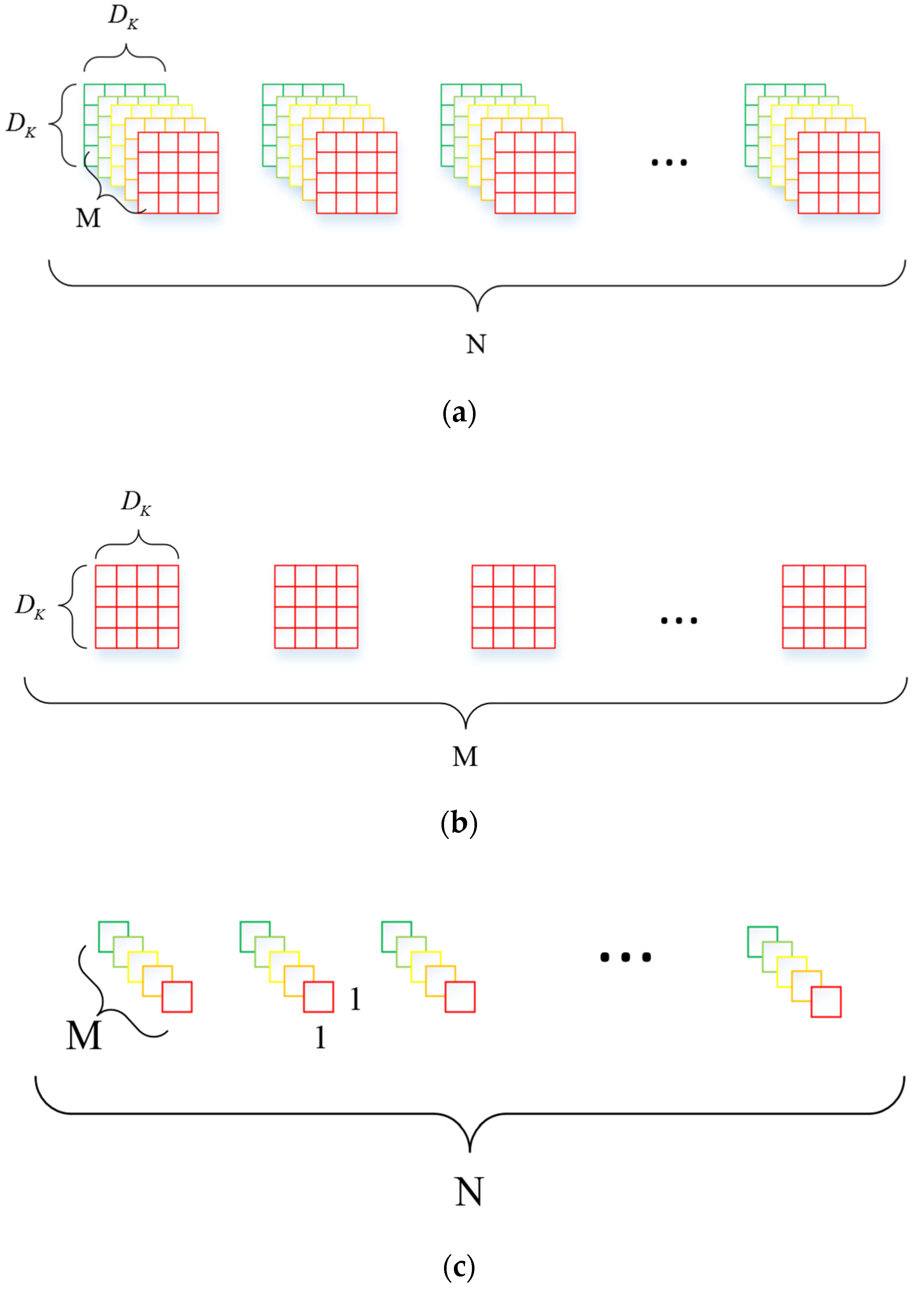
2.1.2. Mobile Net
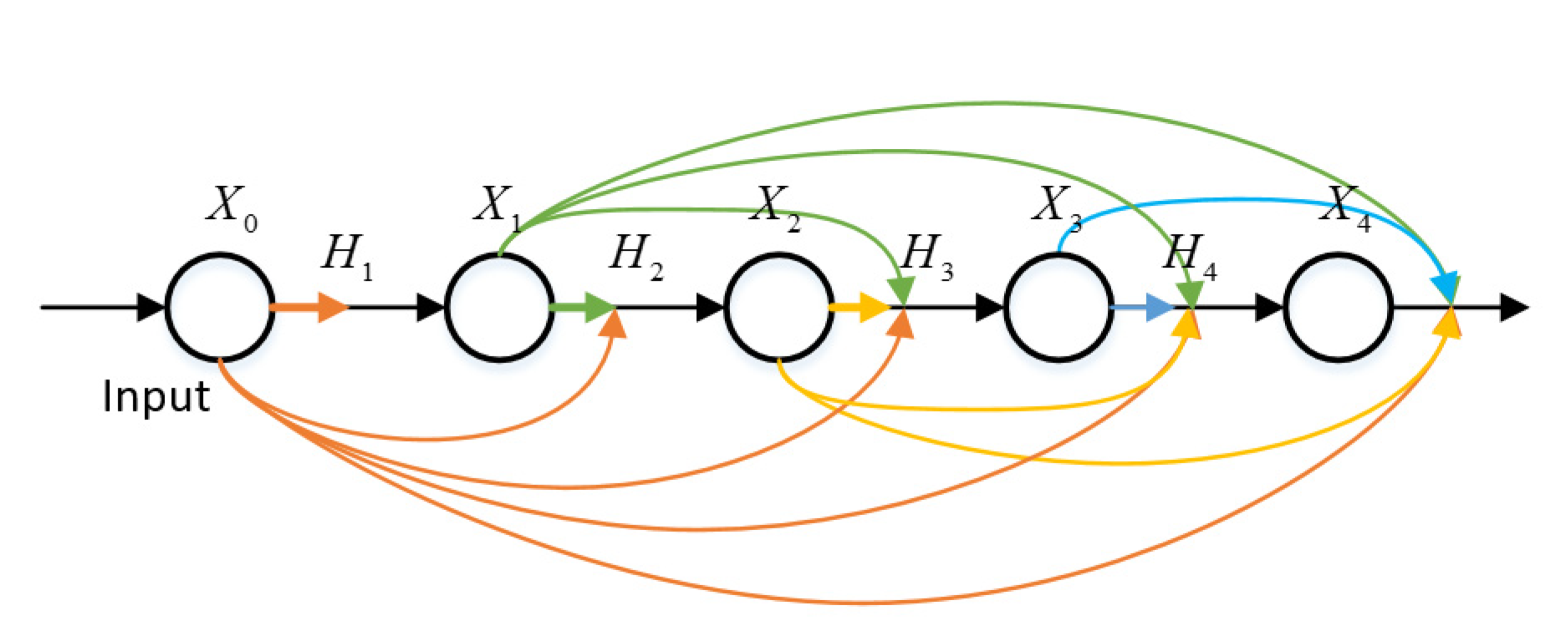
2.1.3. Dense Net
2.2. Feature Transformation
2.2.1. Mean Subtraction
2.2.2. L2-Normalization
2.3. Nearest Neighbor Algorithm
3. Experiments
3.1. Experiment Development
3.2. Results and Analysis
4. Conclusions
Author Contributions
Funding
Data Availability Statement
Conflicts of Interest
References
- Min, S.K.; Taesu, P.; PooGyeon, P. Classification of steel surface defect using convolutional neural network with few images. In Proceedings of the 12th Asian Control Conference (ASCC), Kitakyusyu, Japan, 9–12 June 2019; pp. 1398–1401. [Google Scholar]
- Finn, C.; Abbeel, P.; Levine, S. Model-agnostic meta-learning for fast adaptation of deep networks. arXiv 2018, arXiv:1703.03400. [Google Scholar]
- Ravi, S.; Larochelle, H. Optimization as a model for few-shot learning. In Proceedings of the International Conference on Learning Representations (ICLR), Toulon, France, 24–26 April 2017; pp. 1–11. [Google Scholar]
- Creswell, A.; White, T.; Dumoulin, V.; Arulkumaran, K.; Sengupta, B.; Bharath, A.A. Generative adversarial networks: An overview. IEEE Signal Process Mag. J. 2018, 35, 53–65. [Google Scholar] [CrossRef] [Green Version]
- Wang, X.; Huang, T.E.; Darrell, T.; Gonzalez, J.E.; Yu, F. Frustratingly simple few-shot object detection. arXiv 2020, arXiv:2003.06957. [Google Scholar]
- Sun, B.; Li, B.; Cai, S.C.; Zhang, C. FSCE: Few-shot object detection via contrastive proposal encoding. arXiv 2021, arXiv:2103.05950. [Google Scholar]
- Snell, J.; Swersky, K.; Zemel, R. Prototypical networks for few-shot learning. arXiv 2017, arXiv:1703.05175. [Google Scholar]
- Sung, F.; Yang, Y.X.; Zhang, L.; Xiang, T.; Torr, P.H.; Hospedales, T.M. Learning to compare: Relation ntwork for few-shot learning. arXiv 2017, arXiv:1711.06025. [Google Scholar]
- Koch, G.; Zemel, R.; Salakhutdinov, R. Siamese neural networks for one-shot image recognition. In Proceedings of the Internation Conference on Machine Learning (ICML) Deep Learning Workshop, Lille Grande Palais, Lille, France, 6–11 July 2015; pp. 1–30. [Google Scholar]
- Rusu, A.A.; Rao, D.; Sygnowski, J.; Vinyals, O.; Pascanu, R.; Osindero, S.; Hadsell, R. Meta-learning with latent embedding optimization. arXiv 2019, arXiv:1807.05960. [Google Scholar]
- Maryam, I.; Hassan, G. Band clustering-based feature extraction for classification of hyperspectral images using limited training samples. IEEE Geosci. Remote Sens. Lett. 2014, 11, 1325–1329. [Google Scholar]
- Maryam, I.; Hassan, G. Automatic defect recognition in x-ray testing using computer vision. In Proceedings of the 17th IEEE Winter Conference on Applications of Computer Vision (WACV), Santa Rosa, CA, USA, 24–31 March 2017; pp. 1026–1035. [Google Scholar]
- Maryam, I.; Hassan, G. Feature extraction using attraction points for classification of hyperspectral images in a small sample size situation. IEEE Geosci. Remote Sens. Lett. 2014, 11, 1986–1990. [Google Scholar]
- Zhang, Z.F.; Song, Y.; Cui, H.C.; Wu, J.; Schwartz, F.; Qi, H.R. Topological analysis and Gaussian decision tree: Effective representation and classification of biosignals of small sample size. IEEE Trans. Biomed. Eng. 2017, 64, 2288–2299. [Google Scholar] [CrossRef] [PubMed]
- Fu, G.Z.; Sun, P.; Zhu, W.B.; Yang, J.X.; Yang, M.L.; Cao, Y.P. A deep-learning-based approach for fast and robust steel surface defects classification. Opt. Lasers Eng. 2019, 121, 397–405. [Google Scholar] [CrossRef]
- Krizhevsky, A.; Sutskever, I.; Hinton, G.E. ImageNet classification with deep convolutional neural networks. Adv. Neural Inf. Process. Syst. 2012, 25, 1097–1105. [Google Scholar] [CrossRef]
- Simonyan, K.; Zisserman, A. Very deep convolutional networks for large-scale image recognition. arXiv 2015, arXiv:1409.1556. [Google Scholar]
- Szegedy, C.; Liu, W.; Jia, Y.; Sermanet, P.; Reed, S.; Anguelov, D.; Erhan, D.; Vanhoucke, V.; Rabinovich, A. Going deeper with convolutions. In Proceedings of the IEEE Conference on Computer Vision and Pattern Recognition (CVPR), Boston, MA, USA, 8–10 June 2015; pp. 1–9. [Google Scholar]
- He, K.M.; Zhang, X.Y.; Ren, S.Q.; Sun, J. Deep residual learning for image recognition. In Proceedings of the IEEE Conference on Computer Vision and Pattern Recognition (CVPR), Boston, MA, USA, 8–10 June 2015; pp. 770–778. [Google Scholar]
- Telgarsky, M. Benefits of depth in neural networks. In Proceedings of the Conference on Learning Theory, PMLR, New York, NY, USA, 23–26 June 2016; pp. 1517–1539. [Google Scholar]
- Howard, A.G.; Zhu, M.; Chen, B. Mobilenets: Effificient convolutional neural networks for mobile vision applications. arXiv 2017, arXiv:1704.04861. [Google Scholar]
- Huang, G.; Liu, Z.; Van der Maaten, L.; Weinberger, K. Densely connected convolutional networks. In Proceedings of the IEEE Conference on Computer Vision and Pattern Recognition (CVPR), Honolulu, HI, USA, 22–25 July 2017; pp. 4700–4708. [Google Scholar]
- Wang, Y.; Chao, W.L.; Weinberger, K.Q.; Van der Maaten, L. Simpleshot: Revisiting nearest-neighbor classifification for few-shot learning. arXiv 2019, arXiv:1911.04623. [Google Scholar]


| OS | CPU | GPU | Pytorch | Python |
|---|---|---|---|---|
| Ubuntu 18.04.1 | AMD R9-3900x | RTX 3090 | 1.8.0 | 3.7.0 |
| Net | None | MS | L2 |
|---|---|---|---|
| Convolution4 | 43.67 (0.45) | 49.54 (0.47) | 49.27 (0.46) |
| Residual Net10 | 73.41 (0.40) | 76.14 (0.37) | 78.75 (0.33) |
| Residual Net18 | 56.34 (1.36) | 59.34 (1.39) | 59.33 (1.38) |
| Residual Net34 | 63.42 (1.48) | 65.19 (1.32) | 65.81 (1.33) |
| Residual Net50 | 41.32 (1.53) | 42.68 (1.42) | 45.14 (1.60) |
| Mobile Net | 82.60 (0.57) | 85.78 (0.53) | 87.30 (0.52) |
| Dense Net121 | 82.28 (0.58) | 82.58 (0.49) | 85.16 (0.56) |
| Net | None | MS | L2 |
|---|---|---|---|
| Convolution4 | 62.32 (0.31) | 66.19 (0.30) | 66.24 (0.30) |
| Residual Net10 | 84.62 (0.24) | 85.77 (0.22) | 87.67 (0.20) |
| Residual Net18 | 70.39 (0.95) | 74.54 (0.90) | 74.94 (0.90) |
| Residual Net34 | 71.71 (0.89) | 75.82 (0.86) | 76.02 (0.91) |
| Residual Net50 | 49.60 (1.05) | 54.93 (0.98) | 54.03 (1.06) |
| Mobile Net | 88.27 (0.32) | 90.94 (0.24) | 91.80 (0.23) |
| Dense Net121 | 89.47 (0.31) | 88.97 (0.29) | 92.33 (0.24) |
Publisher’s Note: MDPI stays neutral with regard to jurisdictional claims in published maps and institutional affiliations. |
© 2021 by the authors. Licensee MDPI, Basel, Switzerland. This article is an open access article distributed under the terms and conditions of the Creative Commons Attribution (CC BY) license (https://creativecommons.org/licenses/by/4.0/).
Share and Cite
Wu, S.; Zhao, S.; Zhang, Q.; Chen, L.; Wu, C. Steel Surface Defect Classification Based on Small Sample Learning. Appl. Sci. 2021, 11, 11459. https://doi.org/10.3390/app112311459
Wu S, Zhao S, Zhang Q, Chen L, Wu C. Steel Surface Defect Classification Based on Small Sample Learning. Applied Sciences. 2021; 11(23):11459. https://doi.org/10.3390/app112311459
Chicago/Turabian StyleWu, Shiqing, Shiyu Zhao, Qianqian Zhang, Long Chen, and Chenrui Wu. 2021. "Steel Surface Defect Classification Based on Small Sample Learning" Applied Sciences 11, no. 23: 11459. https://doi.org/10.3390/app112311459