
Attention-Based CNN and Bi-LSTM Model Based on TF-IDF and GloVe Word Embedding for Sentiment Analysis


Abstract
:1. Introduction
- A novel text representation scheme based on TF-IDF feature weighting and pre-trained Glove word embedding has been presented to extract significant features for sentiment analysis.
- We propose a novel attention-based CNN-Bi-LSTM model to improve accuracy and reduce overfitting. The model adopts the advantages of both CNN and LSTM to improve sentiment knowledge and accuracy. To avoid overfitting, we applied Gaussian noise and Gaussian Dropout.
- The attention mechanism is used to pay suitable attention to different words to improve the feature expression ability.
- We performed a comparative experiment on four Twitter datasets to assess the proposed architecture’s effectiveness by improved accuracy.
2. Related Work
2.1. Traditional Sentiment Analysis
2.2. Weighted Word Embedding for Sentiment Analysis
2.3. Deep Models for Sentiment Analysis
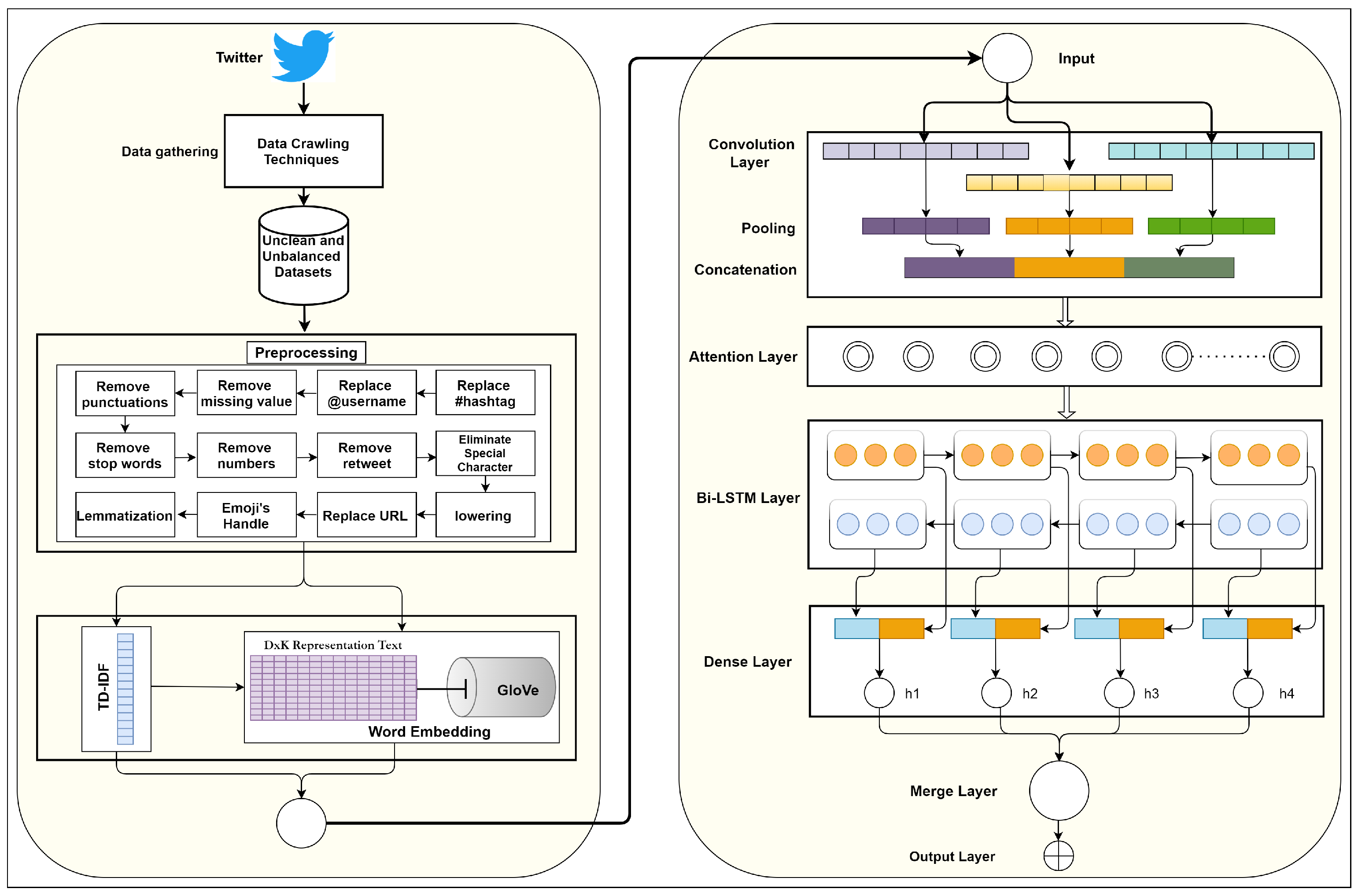
3. Proposed Architecture
3.1. Data Preprocessor
3.2. Weighted Word Representation
3.3. Attention Based Deep Layers
3.4. Full Connection and Output Layer
4. Experiments and Analysis
4.1. Datasets
4.2. Experimental Setup
4.3. Model Variation and Baselines Method
4.4. Results Analysis and Discussion
4.4.1. Analysis of Results on the Sentiment140 Dataset
4.4.2. Analysis of Results on the US-Airline Dataset
4.4.3. Analysis of Results on the Sentiment140-MV Dataset
4.4.4. Analysis of Results on the SD4A Dataset
5. Conclusions
Author Contributions
Funding
Institutional Review Board Statement
Informed Consent Statement
Data Availability Statement
Conflicts of Interest
References
- Abdi, A.; Shamsuddin, S.M.; Hasan, S.; Piran, J. Deep learning-based sentiment classification of evaluative text based on Multi-feature fusion. Inf. Process. Manag. 2019, 56, 1245–1259. [Google Scholar] [CrossRef]
- Chen, M.; Zhou, P.; Wu, D.; Hu, L.; Hassan, M.M.; Alamri, A. AI-Skin: Skin disease recognition based on self-learning and wide data collection through a closed-loop framework. Inf. Fusion 2020, 54, 1–9. [Google Scholar] [CrossRef] [Green Version]
- Tai, K.S.; Socher, R.; Manning, C.D. Improved Semantic Representations From Tree-Structured Long Short-Term Memory Networks. In Proceedings of the 53rd Annual Meeting of the Association for Computational Linguistics and the 7th International Joint Conference on Natural Language Processing, Beijing, China, 26–31 July 2015; Volume 1, pp. 1556–1566. [Google Scholar]
- Er, M.J.; Zhang, Y.; Wang, N.; Pratama, M. Attention pooling-based convolutional neural network for sentence modelling. Inf. Sci. 2016, 373, 388–403. [Google Scholar] [CrossRef]
- Liu, F.; Zheng, J.; Zheng, L.; Chen, C. Combining attention-based bidirectional gated recurrent neural network and two-dimensional convolutional neural network for document-level sentiment classification. Neurocomputing 2020, 371, 39–50. [Google Scholar] [CrossRef]
- Xuanyuan, M.; Xiao, L.; Duan, M. Sentiment Classification Algorithm Based on Multi-Modal Social Media Text Information. IEEE Access 2021, 9, 33410–33418. [Google Scholar] [CrossRef]
- Wang, X.; Liu, Y.C.; Sun, C.J.; Wang, B.X.; Wang, X.L. Predicting Polarities of Tweets by Composing Word Embeddings with Long Short-Term Memory. In Proceedings of the 53rd Annual Meeting of the Association-for-Computational-Linguistics (ACS)/7th International Joint Conference on Natural Language Processing of the Asian-Federation-of-Natural-Language-Processing (IJCNLP), Beijing, China, 26–31 July 2015; pp. 1343–1353. [Google Scholar]
- Siddiqua, U.A.; Chy, A.; Aono, M. Tweet Stance Detection Using Multi-Kernel Convolution and Attentive LSTM Variants. Ieice Trans. Inf. Syst. 2019, E102D, 2493–2503. [Google Scholar] [CrossRef] [Green Version]
- Zhang, C.; Wang, D.; Wang, L.; Song, J.; Liu, S.; Li, J.; Guan, L.; Liu, Z.; Zhang, M. Temporal data-driven failure prognostics using BiGRU for optical networks. J. Opt. Commun. Netw. 2020, 12, 277–287. [Google Scholar] [CrossRef]
- Vaswani, A.; Shazeer, N.; Parmar, N.; Uszkoreit, J.; Jones, L.; Gomez, A.N.; Kaiser, L.; Polosukhin, I. Attention is all you need. arXiv 2017, arXiv:1706.03762. [Google Scholar]
- Song, Y.; Wang, J.; Jiang, T.; Liu, Z.; Rao, Y. Attentional Encoder Network for Targeted Sentiment Classification. arXiv 2019, arXiv:1902.09314. [Google Scholar]
- Usama, M.; Ahmad, B.; Song, E.; Hossain, M.S.; Alrashoud, M.; Muhammad, G. Attention-based sentiment analysis using convolutional and recurrent neural network. Future Gener. Comput.-Syst. Int. J. eSci. 2020, 113, 571–578. [Google Scholar] [CrossRef]
- Rathi, M.; Malik, A.; Varshney, D.; Sharma, R.; Mendiratta, S. Sentiment Analysis of Tweets Using Machine Learning Approach. In Proceedings of the 2018 Eleventh International Conference on Contemporary Computing (IC3), Noida, India, 2–4 August 2018; pp. 1–3. [Google Scholar] [CrossRef]
- Liu, Y.; Jiang, C.; Zhao, H. Assessing product competitive advantages from the perspective of customers by mining user-generated content on social media. Decis. Support Syst. 2019, 123, 113079. [Google Scholar] [CrossRef]
- Saeed, Z.; Ayaz Abbasi, R.; Razzak, I. EveSense: What can you sense from Twitter? In Proceedings of the 42nd European Conference on IR Research, ECIR 2020, Lisbon, Portugal, 14–17 April 2020; Volume 12036 LNCS, Lecture Notes in Computer Science (Including Subseries Lecture Notes in Artificial Intelligence and Lecture Notes in Bioinformatics); Springer Science and Business Media Deutschland GmbH: Berlin/Heidelberg, Germany, 2020; pp. 491–495. [Google Scholar] [CrossRef] [Green Version]
- Saeed, Z.; Ayaz Abbasi, R.; Razzak, M.I.; Xu, G. Event Detection in Twitter Stream Using Weighted Dynamic Heartbeat Graph Approach [Application Notes]. IEEE Comput. Intell. Mag. 2019, 14, 29–38. [Google Scholar] [CrossRef]
- Oliveira, N.; Cortez, P.; Areal, N. Automatic creation of stock market lexicons for sentiment analysis using stocktwits data. In Proceedings of the 18th International Database Engineering and Applications Symposium, IDEAS 2014, Porto, Portugal, 7–9 July 2014; ACM International Conference Proceeding Series; Association for Computing Machinery: New York, NY, USA, 2014; pp. 115–123. [Google Scholar] [CrossRef] [Green Version]
- Rasool, A.; Tao, R.; Kamyab, M.; Hayat, S. GAWA-A Feature Selection Method for Hybrid Sentiment Classification. IEEE Access 2020, 8, 191850–191861. [Google Scholar] [CrossRef]
- Song, C.; Wang, X.K.; Cheng, P.F.; Wang, J.Q.; Li, L. SACPC: A framework based on probabilistic linguistic terms for short text sentiment analysis. Knowl.-Based Syst. 2020, 194, 105572. [Google Scholar] [CrossRef]
- Sun, S.; Luo, C.; Chen, J. A review of natural language processing techniques for opinion mining systems. Inf. Fusion 2017, 36, 10–25. [Google Scholar] [CrossRef]
- Arun, C.; Karthick, S.; Selvakumarasamy, S.; Joseph James, S. Car parking location tracking, routing and occupancy monitoring system using cloud infrastructure. Mater. Today Proc. 2021. [Google Scholar] [CrossRef]
- Rubtsova, Y. Automatic Term Extraction for Sentiment Classification of Dynamically Updated Text Collections into Three Classes. In Knowledge Engineering and the Semantic Web; Klinov, P., Mouromtsev, D., Eds.; Springer International Publishing: Cham, Switzerland, 2014; pp. 140–149. [Google Scholar]
- Chen, X.; Tang, W.; Xu, H.; Hu, X. Double LDA: A Sentiment Analysis Model Based on Topic Model. In Proceedings of the 2014 10th International Conference on Semantics, Knowledge and Grids, Beijing, China, 25–29 August 2014; pp. 49–56. [Google Scholar] [CrossRef]
- Fu, X.; Liu, W.; Xu, Y.; Cui, L. Combine HowNet lexicon to train phrase recursive autoencoder for sentence-level sentiment analysis. Neurocomputing 2017, 241, 18–27. [Google Scholar] [CrossRef]
- Qin, P.; Xu, W.; Guo, J. An empirical convolutional neural network approach for semantic relation classification. Neurocomputing 2016, 190, 1–9. [Google Scholar] [CrossRef]
- Abid, F.; Alam, M.; Yasir, M.; Li, C. Sentiment analysis through recurrent variants latterly on convolutional neural network of Twitter. Future Gener. Comput.-Syst. Int. J. eSci. 2019, 95, 292–308. [Google Scholar] [CrossRef]
- Zhao, J.; Gui, X.; Zhang, X. Deep Convolution Neural Networks for Twitter Sentiment Analysis. IEEE Access 2018, 6, 23253–23260. [Google Scholar] [CrossRef]
- Araque, O.; Corcuera-Platas, I.; Sánchez-Rada, J.F.; Iglesias, C.A. Enhancing deep learning sentiment analysis with ensemble techniques in social applications. Expert Syst. Appl. 2017, 77, 236–246. [Google Scholar] [CrossRef]
- Kamkarhaghighi, M.; Makrehchi, M. Content Tree Word Embedding for document representation. Expert Syst. Appl. 2017, 90, 241–249. [Google Scholar] [CrossRef]
- Zhao, R.; Mao, K. Fuzzy Bag-of-Words Model for Document Representation. IEEE Trans. Fuzzy Syst. 2018, 26, 794–804. [Google Scholar] [CrossRef]
- Chen, G.; Xiao, L. Selecting publication keywords for domain analysis in bibliometrics: A comparison of three methods. J. Inf. 2016, 10, 212–223. [Google Scholar] [CrossRef]
- Hu, K.; Wu, H.; Qi, K.; Yu, J.; Yang, S.; Yu, T.; Zheng, J.; Liu, B. A domain keyword analysis approach extending Term Frequency-Keyword Active Index with Google Word2Vec model. Scientometrics 2018, 114, 1031–1068. [Google Scholar] [CrossRef]
- Stelzer, F.; Röhm, A.; Vicente, R.; Fischer, I.; Yanchuk, S. Deep neural networks using a single neuron: Folded-in-time architecture using feedback-modulated delay loops. Nat. Commun. 2021, 12, 5164. [Google Scholar] [CrossRef]
- Dang, N.C.; Moreno-Garcia, M.N.; De la Prieta, F. Sentiment Analysis Based on Deep Learning: A Comparative Study. Electronics 2020, 9, 483. [Google Scholar] [CrossRef] [Green Version]
- Johnson, R.; Zhang, T. Deep pyramid convolutional neural networks for text categorization. In Proceedings of the 55th Annual Meeting of the Association for Computational Linguistics, ACL 2017, Vancouver, BC, Canada, 30 July–4 August 2017; Association for Computational Linguistics (ACL): Stroudsburg, PA, USA, 2017; Volume 1, pp. 562–570. [Google Scholar] [CrossRef] [Green Version]
- Rezaeinia, S.M.; Rahmani, R.; Ghodsi, A.; Veisi, H. Sentiment analysis based on improved pre-trained word embeddings. Expert Syst. Appl. 2019, 117, 139–147. [Google Scholar] [CrossRef]
- Dos Santos, C.N.; Gatti, M. Deep convolutional neural networks for sentiment analysis of short texts. In Proceedings of the 25th International Conference on Computational Linguistics, Dublin, Ireland, 23–29 August 2014; pp. 69–78. [Google Scholar]
- Wang, J.; Yu, L.C.; Lai, K.R.; Zhang, X. Dimensional sentiment analysis using a regional CNN-LSTM model. In Proceedings of the 54th Annual Meeting of the Association for Computational Linguistics, ACL 2016, Berlin, Germany, 7–12 August 2016; pp. 225–230. [Google Scholar] [CrossRef]
- Yoon, J.; Kim, H. Multi-channel lexicon integrated CNN-BILSTM models for sentiment analysis. In Proceedings of the 29th Conference on Computational Linguistics and Speech Processing, ROCLING 2017, Taipei, Taiwan, 27–28 November 2017; pp. 244–253. [Google Scholar]
- Nguyen, H.T.; Nguyen, M.L. An ensemble method with sentiment features and clustering support. Neurocomputing 2019, 370, 155–165. [Google Scholar] [CrossRef]
- Chatterjee, A.; Gupta, U.; Chinnakotla, M.K.; Srikanth, R.; Galley, M.; Agrawal, P. Understanding Emotions in Text Using Deep Learning and Big Data. Comput. Hum. Behav. 2019, 93, 309–317. [Google Scholar] [CrossRef]
- Liu, G.; Guo, J. Bidirectional LSTM with attention mechanism and convolutional layer for text classification. Neurocomputing 2019, 337, 325–338. [Google Scholar] [CrossRef]
- Wen, S.; Li, J. Recurrent convolutional neural network with attention for twitter and yelp sentiment classification arc model for sentiment classification. In Proceedings of the 2018 International Conference on Algorithms, Computing and Artificial Intelligence, ACAI 2018, Sanya, China, 21–23 December 2018; The Hong Kong Polytechnic University: Hong Kong, China, 2018. [Google Scholar] [CrossRef]
- Basiri, M.E.; Nemati, S.; Abdar, M.; Cambria, E.; Acharrya, U.R. ABCDM: An Attention-based Bidirectional CNN-RNN Deep Model for sentiment analysis. Future Gener. Comput. Syst. 2021, 115, 279–294. [Google Scholar] [CrossRef]
- Li, W.; Qi, F.; Tang, M.; Yu, Z. Bidirectional LSTM with self-attention mechanism and multi-channel features for sentiment classification. Neurocomputing 2020, 387, 63–77. [Google Scholar] [CrossRef]
- Kumawat, S.; Yadav, I.; Pahal, N.; Goel, D. Sentiment Analysis Using Language Models: A Study. In Proceedings of the 11th International Conference on Cloud Computing, Data Science and Engineering (Confluence), Noida, India, 28–29 January 2021; pp. 984–988. [Google Scholar] [CrossRef]
- Sun, C.; Huang, L.; Qiu, X. Utilizing BERT for Aspect-Based Sentiment Analysis via Constructing Auxiliary Sentence. arXiv 2019, arXiv:1903.09588. [Google Scholar]
- Wang, S.; Fang, H.; Khabsa, M.; Mao, H.; Ma, H. Entailment as Few-Shot Learner. arXiv 2021, arXiv:2104.14690. [Google Scholar]
- Onan, A.; Tocoglu, M.A. A Term Weighted Neural Language Model and Stacked Bidirectional LSTM Based Framework for Sarcasm Identification. IEEE Access 2021, 9, 7701–7722. [Google Scholar] [CrossRef]
- Yu, L.C.; Wang, J.; Lai, K.R.; Zhang, X. Refining Word Embeddings Using Intensity Scores for Sentiment Analysis. IEEE/ACM Trans. Audio Speech Lang. Process. 2018, 26, 671–681. [Google Scholar] [CrossRef]
- Go, A.; Bhayani, R.; Huang, L. Twitter Sentiment Classification Using Distant Supervision. CS224N Project Report, Stanford. 2009. Available online: https://cs.stanford.edu/people/alecmgo/papers/TwitterDistantSupervision09.pdf (accessed on 20 October 2021).
- Kamyab, M.; Tao, R.; Mohammadi, M.H.; Rasool, A. Sentiment analysis on Twitter: A text mining approach to the Afghanistan status reviews. In Proceedings of the 2018 International Conference on Artificial Intelligence and Virtual Reality, AIVR 2018, Nagoya, Japan, 23–25 November 2018; Association for Computing Machinery: New York, NY, USA, 2018; pp. 14–19. [Google Scholar] [CrossRef]
- Socher, R.; Perelygin, A.; Wu, J.Y.; Chuang, J.; Manning, C.D.; Ng, A.Y.; Potts, C. Recursive deep models for semantic compositionality over a sentiment treebank. In Proceedings of the 2013 Conference on Empirical Methods in Natural Language Processing, EMNLP 2013, Seattle, WA, USA, 18–21 October 2013; Association for Computational Linguistics (ACL): Stroudsburg, PA, USA, 2013; pp. 1631–1642. [Google Scholar]
- Subba, B.; Kumari, S. A heterogeneous stacking ensemble based sentiment analysis framework using multiple word embeddings. Comput. Intell. 2021. Early Access. [Google Scholar] [CrossRef]
- Yang, Z.; Yang, D.; Dyer, C.; He, X.; Smola, A.; Hovy, E. Hierarchical attention networks for document classification. In Proceedings of the 15th Conference of the North American Chapter of the Association for Computational Linguistics: Human Language Technologies, NAACL HLT 2016, San Diego, CA, USA, 12–17 June 2016; Association for Computational Linguistics (ACL): Stroudsburg, PA, USA, 2016; pp. 1480–1489. [Google Scholar]


| Dataset | Max | Min | Avg | Positive | Negative | Total |
|---|---|---|---|---|---|---|
| SD4A | 38 | 4 | 16 | 18,309 | 18,539 | 36,848 |
| Sentiment140 | 40 | 1 | 12 | 248,576 | 80,000 | 1,048,576 |
| Sentiment140-MV | 35 | 3 | 15 | 11,628 | 6585 | 18,213 |
| US Airline | 30 | 1 | 15.5 | 2343 | 9112 | 11,455 |
| Proposed | Narrative |
|---|---|
| TF-IDF-Glove-CNN | |
| TF-IDF-Glove-LSTM | |
| TF-IDF-Glove-BiLSTM | Methods used TF-IDF-Glove word embedding. |
| TF-IDF-Glove-CNN-LSTM | |
| TF-IDF-Glove-CNN-BiLSTM |
| Author/Year | Models | Accuracy |
|---|---|---|
| Li et al. [53] | RNTN | 0.8070 |
| Li et al. [37] | CharSCNN | 0.8570 |
| Wang et al. [38] | CRNN | 0.7987 |
| Nguyen & Nguyen [40] | CNN autoencoder | 0.7931 |
| Nguyen & Nguyen [40] | BiLSTM autoencoder | 0.7911 |
| Rezaeinia et al. [36] | IWV | 0.8052 |
| Song et al. [19] | SAPCP | 0.8522 |
| Dang et al. [34] | TF-IDF-CNN | 0.7668 |
| Dang et al. [34] | TF-IDF-RNN | 0.5695 |
| Dang et al. [34] | Word embeeding -CNN | 0.8006 |
| Dang et al. [34] | Word embeeding -RNN | 0.8281 |
| Basiri et al. [44] | ABCDM | 0.8182 |
| Subba and Kumari [54] | BERT-GloVe-Word2Vec-BiRNN | 0.84 |
| Wang et al. [48] | EFL | 0.863 |
| TF-IDF-Glove-LSTM | 0.8234 | |
| TF-IDF-Glove-BiLSTM | 0.8345 | |
| TF-IDF-Glove-CNN | 0.8322 | |
| TF-IDF-GloveLSTM+CNN | 0.8432 | |
| TF-IDF-Glove-BILSTM-CNN | 0.8530 | |
| Our model | ACL-SA | 0.8712 |
| Author/Year | Models | Accuracy |
|---|---|---|
| Li et al. [53] | CharSCNN | 0.865 |
| Kumawat et al. [46] | BERT-DNN | 0.81 |
| Wang et al. [38] | CRNN | 0.9205 |
| Yang et al. [55] | HAN | 0.9035 |
| Jianqiang et al. [27] | Glove-DCNN | 0.839 |
| Wen & Li [43] | ARC | 0.9229 |
| Rezaeinia et al. [36] | IVM | 0.8985 |
| Chatterjee et al. [41] | SS-BED | 0.91 |
| Liu & Guo [42] | AC-BiLSTM | 0.9172 |
| Dang et al. [34] | TF-IDF-CNN | 0.6879 |
| Dang et al. [34] | TF-IDF-RNN | 0.6174 |
| Dang et al. [34] | Word embeeding-CNN | 0.8236 |
| Dang et al. [34] | Word embeeding-RNN | 0.8376 |
| Basiri et al. [44] | ABCDM | 0.9275 |
| Wang et al. [48] | EFL | 0.9208 |
| TF-IDF-Glove-LSTM | 0.9041 | |
| TF-IDF-Glove-BiLSTM | 0.913 | |
| TF-IDF-Glove-CNN | 0.9198 | |
| TF-IDF-Glove-LSTM+CNN | 0.9189 | |
| TF-IDF-Glove-BILSTM-CNN | 0.9358 | |
| Our model | ACL-SA | 0.9401 |
| Models | Accuracy | Average Accuracy |
|---|---|---|
| TFIDF with DT | 0.7568 | 0.812475 |
| TFIDF with RF | 0.8589 | |
| TFIDF with SVM | 0.8621 | |
| TFIDF with NB | 0.7721 | |
| TF-IDF-Glove-LSTM | 0.9075 | 0.9194 |
| TF-IDF-Glove-BiLSTM | 0.9090 | |
| TF-IDF-Glove-CNN | 0.9141 | |
| TF-IDF-Glove-LSTM-CNN | 0.9369 | |
| TF-IDF-Glove-BILSTM+CNN | 0.9370 | |
| ACL-SA | 0.9443 | 0.9443 |
| Models | Accuracy | Average Accuracy |
|---|---|---|
| TFIDF with DT | 0.7391 | 0.828225 |
| TFIDF with RF | 0.8592 | |
| TFIDF with SVM | 0.8621 | |
| TFIDF with NB | 0.8525 | |
| TF-IDF Glove-LSTM | 0.9141 | 0.9207 |
| TF-IDF Glove-BiLSTM | 0.911 | |
| TF-IDF Glove-CNN | 0.9209 | |
| TF-IDF Glove-LSTM-CNN | 0.9238 | |
| TF-IDF Glove-BILSTM+CNN | 0.9337 | |
| ACL-SA | 0.9453 | 0.9453 |
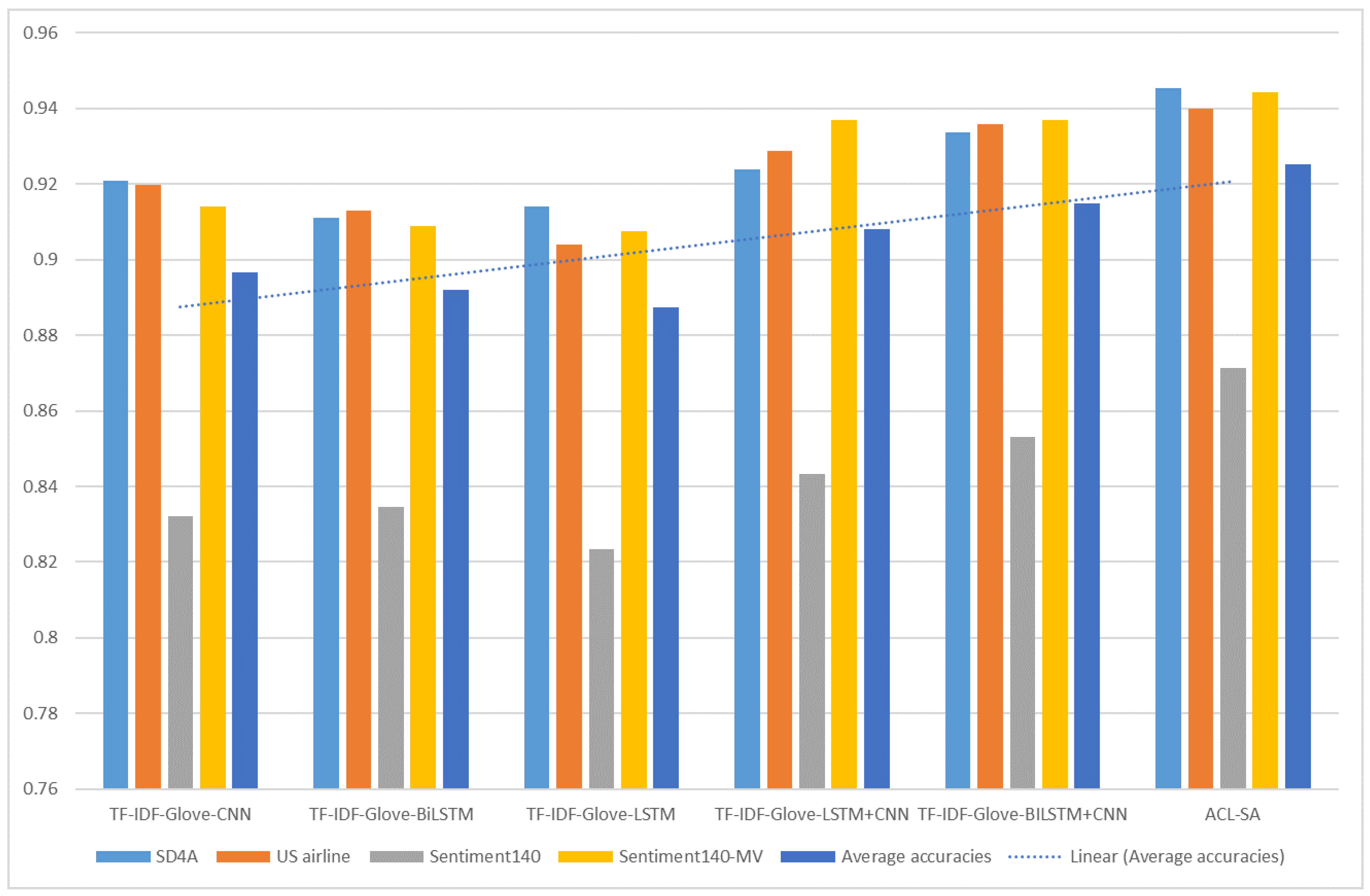
| Dataset | TF-IDF-Glove-CNN | TF-IDF-Glove-BiLSTM | TF-IDF-Glove-LSTM | TF-IDF-Glove-LSTM+CNN | TF-IDF-GloVe-BILSTM+CNN | ACL-SA |
| SD4A | 0.9209 | 0.911 | 0.9141 | 0.9238 | 0.9337 | 0.9453 |
| US airline | 0.9198 | 0.913 | 0.9041 | 0.9289 | 0.9358 | 0.94 |
| Sentiment140 | 0.8322 | 0.8345 | 0.8234 | 0.8432 | 0.853 | 0.8712 |
| Sentiment140-MV | 0.9141 | 0.909 | 0.9075 | 0.9369 | 0.937 | 0.9443 |
| Average accuracies | 0.8967 | 0.8919 | 0.8873 | 0.9082 | 0.91499 | 0.9252 |
| Measure | Dataset | Comparison | Hypothesis | p-Value |
|---|---|---|---|---|
| Classification accuracy | US-airline | ACL-SA vs. ABCDM | Rejected for ACL-SA | 0.003 |
| ACL-SA vs. CRNN | Rejected for ACL-SA | 0.025 | ||
| ACL-SA vs. ACR | Rejected for ACL-SA | 0.025 | ||
| ACL-SA vs. IVM | Rejected for ACL-SA | 0.026 | ||
| ACL-SA vs. SS-BED | Rejected for ACL-SA | 0.024 | ||
| ACL-SA vs. AC-BiLSTM | Rejected for ACL-SA | 0.016 | ||
| ACL-SA vs. Word Embeeding-RNN | Rejected for ACL-SA | 0.031 | ||
| Sentiment140 | ACL-SA vs. CRNN | Rejected for ACL-SA | 0.001 | |
| ACL-SA vs. IWV | Rejected for ACL-SA | 0.011 | ||
| ACL-SA vs. SAPCP | Rejected for ACL-SA | 0.001 | ||
| ACL-SA vs. Word Embedding-RNN | Rejected for ACL-SA | 0.001 | ||
| ACL-SA vs. ABCDM | Rejected for ACL-SA | 0.005 |
Publisher’s Note: MDPI stays neutral with regard to jurisdictional claims in published maps and institutional affiliations. |
© 2021 by the authors. Licensee MDPI, Basel, Switzerland. This article is an open access article distributed under the terms and conditions of the Creative Commons Attribution (CC BY) license (https://creativecommons.org/licenses/by/4.0/).
Share and Cite
Kamyab, M.; Liu, G.; Adjeisah, M. Attention-Based CNN and Bi-LSTM Model Based on TF-IDF and GloVe Word Embedding for Sentiment Analysis. Appl. Sci. 2021, 11, 11255. https://doi.org/10.3390/app112311255
Kamyab M, Liu G, Adjeisah M. Attention-Based CNN and Bi-LSTM Model Based on TF-IDF and GloVe Word Embedding for Sentiment Analysis. Applied Sciences. 2021; 11(23):11255. https://doi.org/10.3390/app112311255
Chicago/Turabian StyleKamyab, Marjan, Guohua Liu, and Michael Adjeisah. 2021. "Attention-Based CNN and Bi-LSTM Model Based on TF-IDF and GloVe Word Embedding for Sentiment Analysis" Applied Sciences 11, no. 23: 11255. https://doi.org/10.3390/app112311255