
Ensemble-Guided Model for Performance Enhancement in Model-Complexity-Limited Acoustic Scene Classification

 ,
,
Abstract
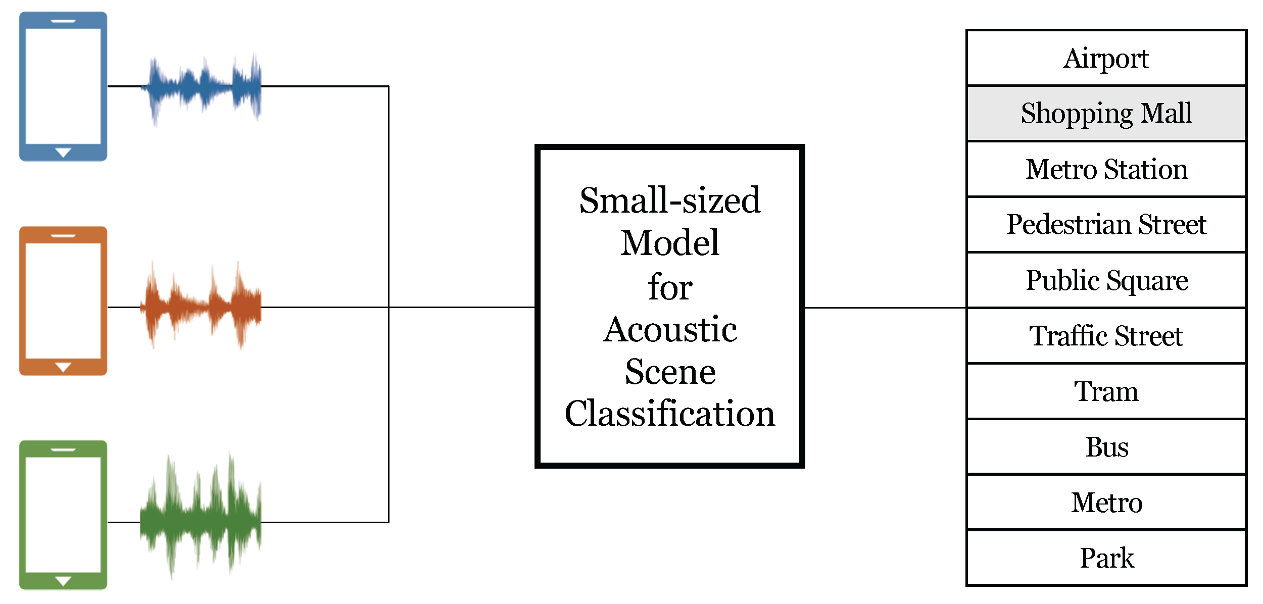
:1. Introduction
2. Problem Description
3. Ensemble-Guided Models
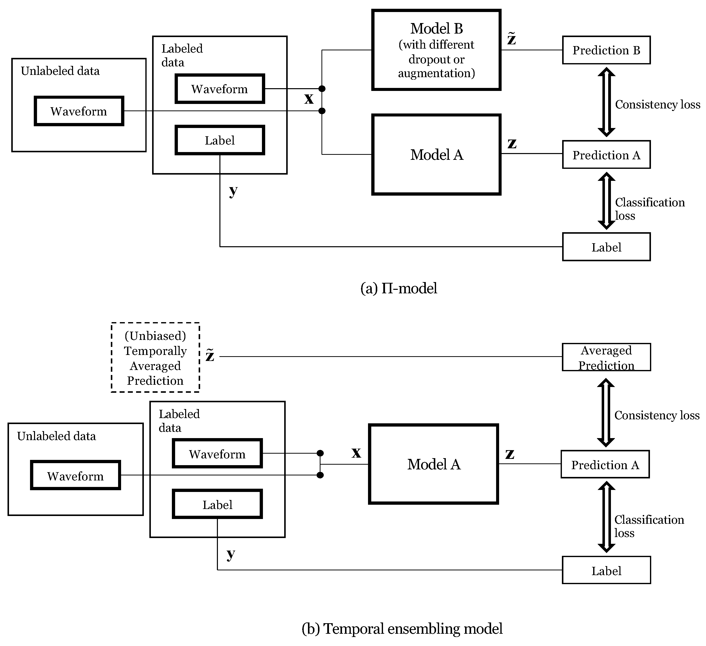
3.1. -Model and Temporal Ensembling for Semi-Supervised Learning
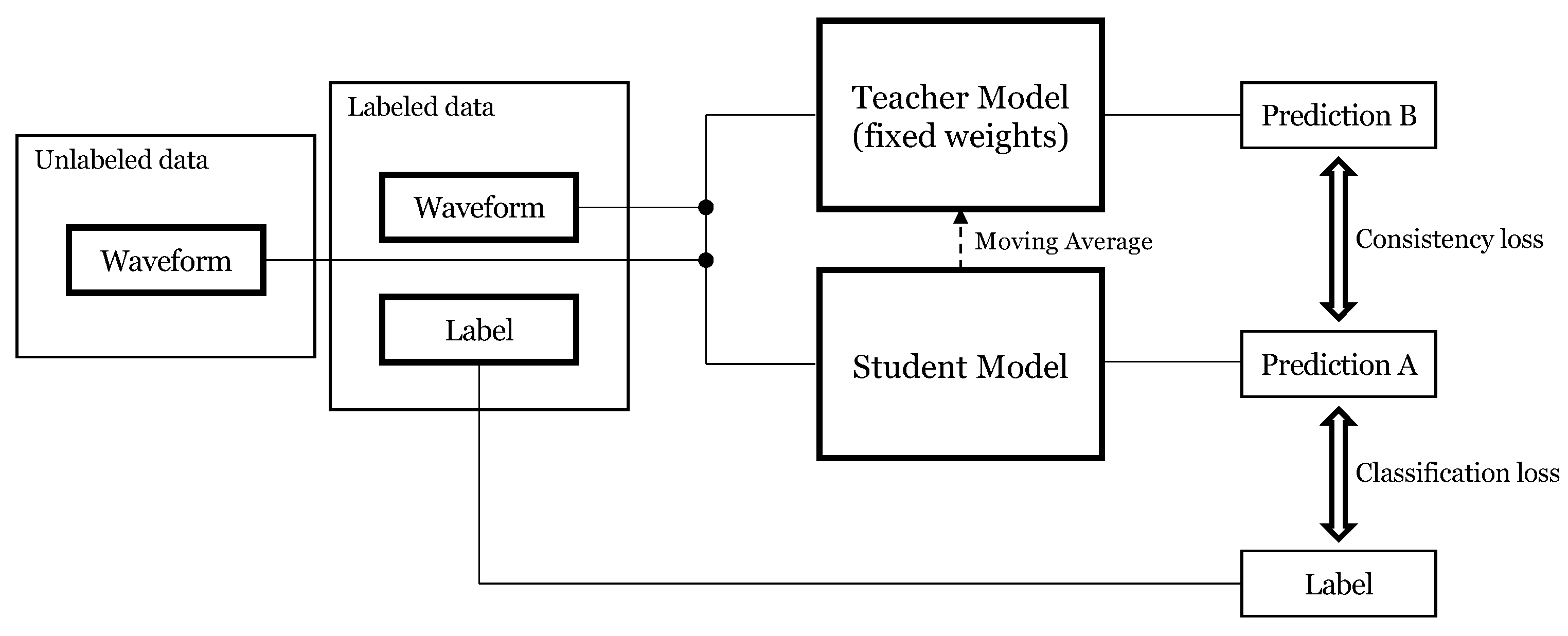
3.2. Mean-Teacher Model for Semi-Supervised Learning
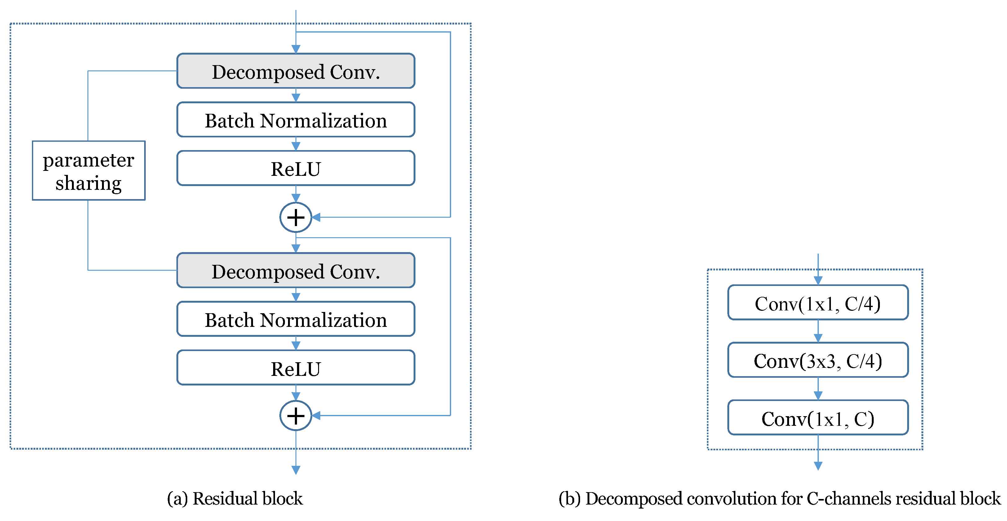
3.3. Proposed Ensemble-Guided Model for Model-Complexity-Limited ASC
4. Evaluation
4.1. Evaluation Settings
4.2. Performance Comparison with Other Ensemble-Guided and Vanilla Models
4.3. Performance Comparison with Various Parameters
4.4. Application to State-of-the-Art Model
5. Conclusions
Author Contributions
Funding
Institutional Review Board Statement
Informed Consent Statement
Data Availability Statement
Conflicts of Interest
Abbreviations
| ASC | Acoustic scene classification |
| CNN | Convolutional neural network |
| CP | Canonical polyadic |
| DCASE | Detection and classification of acoustic scenes and events |
| SED | Sound event detection |
| WRN | Wide ResNet |
References
- Chu, S.; Narayanan, S.; Kuo, C.C.J.; Mataric, M.J. Where am I? Scene recognition for mobile robots using audio features. In Proceedings of the 2006 IEEE International Conference on Multimedia and Expo, Toronto, ON, Canada, 9–12 July 2006; IEEE: Piscataway, NJ, USA, 2006; pp. 885–888. [Google Scholar]
- Ellis, D.P.; Lee, K. Minimal-impact audio-based personal archives. In Proceedings of the the 1st ACM workshop on Continuous Archival and Retrieval of Personal Experiences, New York, NY, USA, 15 October 2004; pp. 39–47. [Google Scholar]
- Barchiesi, D.; Giannoulis, D.; Stowell, D.; Plumbley, M.D. Acoustic scene classification: Classifying environments from the sounds they produce. IEEE Signal Process. Mag. 2015, 32, 16–34. [Google Scholar] [CrossRef]
- Mesaros, A.; Heittola, T.; Virtanen, T. A multi-device dataset for urban acoustic scene classification. arXiv 2018, arXiv:1807.09840. [Google Scholar]
- Koizumi, Y.; Saito, S.; Uematsu, H.; Harada, N.; Imoto, K. ToyADMOS: A dataset of miniature-machine operating sounds for anomalous sound detection. In Proceedings of the 2019 IEEE Workshop on Applications of Signal Processing to Audio and Acoustics (WASPAA), New Paltz, NY, USA, 20–23 October 2019; IEEE: Piscataway, NJ, USA, 2019; pp. 313–317. [Google Scholar]
- Lee, S.; Pang, H.S. Feature extraction based on the non-negative matrix factorization of convolutional neural networks for monitoring domestic activity with acoustic signals. IEEE Access 2020, 8, 122384–122395. [Google Scholar] [CrossRef]
- Politis, A.; Adavanne, S.; Krause, D.; Deleforge, A.; Srivastava, P.; Virtanen, T. A Dataset of Dynamic Reverberant Sound Scenes with Directional Interferers for Sound Event Localization and Detection. arXiv 2021, arXiv:2106.06999. [Google Scholar]
- Amiriparian, S.; Gerczuk, M.; Ottl, S.; Cummins, N.; Freitag, M.; Pugachevskiy, S.; Baird, A.; Schuller, B. Snore sound classification using image-based deep spectrum features. In Proceedings of the Interspeech, Stockholm, Sweden, 20–24 August 2017; pp. 3512–3516. [Google Scholar]
- Połap, D.; Woźniak, M.; Damaševičius, R.; Maskeliūnas, R. Bio-inspired voice evaluation mechanism. Appl. Soft Comput. 2019, 80, 342–357. [Google Scholar] [CrossRef]
- Sawhney, N.; Maes, P. Situational awareness from environmental sounds. Proj. Rep. Pattie Maes 1997, 1–7. Available online: https://www.researchgate.net/profile/Nitin-Sawhney/publication/2796654_Situational_Awareness_from_Environmental_Sounds/links/551984bc0cf2f51a6fe9dd62/Situational-Awareness-from-Environmental-Sounds.pdf (accessed on 15 December 2021).
- Clarkson, B.; Sawhney, N.; Pentland, A. Auditory context awareness via wearable computing. Energy 1998, 400, 20. [Google Scholar]
- Suh, S.; Park, S.; Jeong, Y.; Lee, T. Designing Acoustic Scene Classification Models with CNN Variants. Technical Report. In Proceedings of the DCASE2020 Challenge, online, 1 July 2020. [Google Scholar]
- Yang, C.H.H.; Hu, H.; Siniscalchi, S.M.; Wang, Q.; Yuyang, W.; Xia, X.; Zhao, Y.; Wu, Y.; Wang, Y.; Du, J.; et al. A Lottery Ticket Hypothesis Framework for Low-Complexity Device-Robust Neural Acoustic Scene Classification. Technical Report. In Proceedings of the DCASE2021 Challenge, online, 1 July 2021. [Google Scholar]
- Koutini, K.; Jan, S.; Widmer, G. Cpjku Submission to Dcase21: Cross-Device Audio Scene Classification with Wide Sparse Frequency-Damped CNNs. Technical Report. In Proceedings of the DCASE2021 Challenge, online, 1 July 2021. [Google Scholar]
- He, K.; Zhang, X.; Ren, S.; Sun, J. Deep residual learning for image recognition. In Proceedings of the IEEE Conference on Computer Vision and Pattern Recognition, Las Vegas, NV, USA, 27–30 June 2016; pp. 770–778. [Google Scholar]
- Szegedy, C.; Vanhoucke, V.; Ioffe, S.; Shlens, J.; Wojna, Z. Rethinking the inception architecture for computer vision. In Proceedings of the IEEE Conference on Computer Vision and Pattern Recognition, Las Vegas, NV, USA, 27–30 June 2016; pp. 2818–2826. [Google Scholar]
- Hu, H.; Yang, C.H.H.; Xia, X.; Bai, X.; Tang, X.; Wang, Y.; Niu, S.; Chai, L.; Li, J.; Zhu, H.; et al. Device-Robust Acoustic Scene Classification Based on Two-Stage Categorization and Data Augmentation. Technical Report. In Proceedings of the DCASE2020 Challenge, online, 1 July 2020. [Google Scholar]
- Gao, W.; McDonnell, M. Acoustic Scene Classification Using Deep Residual Networks with Focal Loss and Mild Domain Adaptation. Technical Report. In Proceedings of the DCASE2020 Challenge, online, 1 July 2020. [Google Scholar]
- Turpault, N.; Serizel, R.; Parag Shah, A.; Salamon, J. Sound event detection in domestic environments with weakly labeled data and soundscape synthesis. In Proceedings of the Workshop on Detection and Classification of Acoustic Scenes and Events, New York, NY, USA, 25–26 October 2019. [Google Scholar]
- Martín-Morató, I.; Heittola, T.; Mesaros, A.; Virtanen, T. Low-complexity acoustic scene classification for multi-device audio: Analysis of DCASE 2021 Challenge systems. arXiv 2021, arXiv:2105.13734. [Google Scholar]
- Liu, Y.; Liang, J.; Zhao, L.; Liu, J.; Zhao, K.; Liu, W.; Zhang, L.; Xu, T.; Shi, C. DCASE 2021 Task 1 Subtask A: Low-Complexity Acoustic Scene Classification. Technical Report. In Proceedings of the DCASE2021 Challenge, online, 1 July 2021. [Google Scholar]
- Koutini, K.; Henkel, F.; Eghbal-zadeh, H.; Widmer, G. CP-JKU Submissions to DCASE’20: Low-Complexity Cross-Device Acoustic Scene Classification with RF-Regularized CNNs. Technical Report. In Proceedings of the DCASE2020 Challenge, online, 1 July 2020. [Google Scholar]
- Liu, Z.; Sun, M.; Zhou, T.; Huang, G.; Darrell, T. Rethinking the value of network pruning. arXiv 2018, arXiv:1810.05270. [Google Scholar]
- Laine, S.; Aila, T. Temporal ensembling for semi-supervised learning. arXiv 2016, arXiv:1610.02242. [Google Scholar]
- Tarvainen, A.; Valpola, H. Mean teachers are better role models: Weight-averaged consistency targets improve semi-supervised deep learning results. arXiv 2017, arXiv:1703.01780. [Google Scholar]
- Stowell, D.; Giannoulis, D.; Benetos, E.; Lagrange, M.; Plumbley, M.D. Detection and classification of acoustic scenes and events. IEEE Trans. Multimed. 2015, 17, 1733–1746. [Google Scholar] [CrossRef]
- Heittola, T.; Mesaros, A.; Virtanen, T. Acoustic scene classification in dcase 2020 challenge: Generalization across devices and low complexity solutions. arXiv 2020, arXiv:2005.14623. [Google Scholar]
- Kim, B.; Chang, S.; Lee, J.; Sung, D. Broadcasted Residual Learning for Efficient Keyword Spotting. arXiv 2021, arXiv:2106.04140. [Google Scholar]
- Hu, J.; Shen, L.; Sun, G. Squeeze-and-excitation networks. In Proceedings of the IEEE Conference on Computer Vision and Pattern Recognition, Salt Lake City, UT, USA, 18–23 June 2018; pp. 7132–7141. [Google Scholar]
- Wu, J.; Wang, Y.; Wu, Z.; Wang, Z.; Veeraraghavan, A.; Lin, Y. Deep k-means: Re-training and parameter sharing with harder cluster assignments for compressing deep convolutions. In Proceedings of the International Conference on Machine Learning, PMLR, Stockholm, Sweden, 10–15 July 2018; pp. 5363–5372. [Google Scholar]
- Ruder, S. An overview of gradient descent optimization algorithms. arXiv 2016, arXiv:1609.04747. [Google Scholar]
- Pedregosa, F.; Varoquaux, G.; Gramfort, A.; Michel, V.; Thirion, B.; Grisel, O.; Blondel, M.; Prettenhofer, P.; Weiss, R.; Dubourg, V.; et al. Scikit-learn: Machine Learning in Python. J. Mach. Learn. Res. 2011, 12, 2825–2830. [Google Scholar]
- Heo, H.-S.; Jung, J.-w.; Shim, H.-j.; Lee, B.-J. Clova submission for the DCASE 2021 challenge: Acoustic scene classification using light architectures and device augmentation. Technical Report. In Proceedings of the DCASE2021 Challenge, online, 1 July 2021. [Google Scholar]
- McDonnell, M.D. Training wide residual networks for deployment using a single bit for each weight. arXiv 2018, arXiv:1802.08530. [Google Scholar]
- Kim, B.; Yang, S.; Kim, J.; Chang, S. QTI submission to DCASE 2021: Residual normalization for device imbalanced acoustic scene classification with efficient design. Technical Report. In Proceedings of the DCASE2021 Challenge, online, 1 July 2021. [Google Scholar]


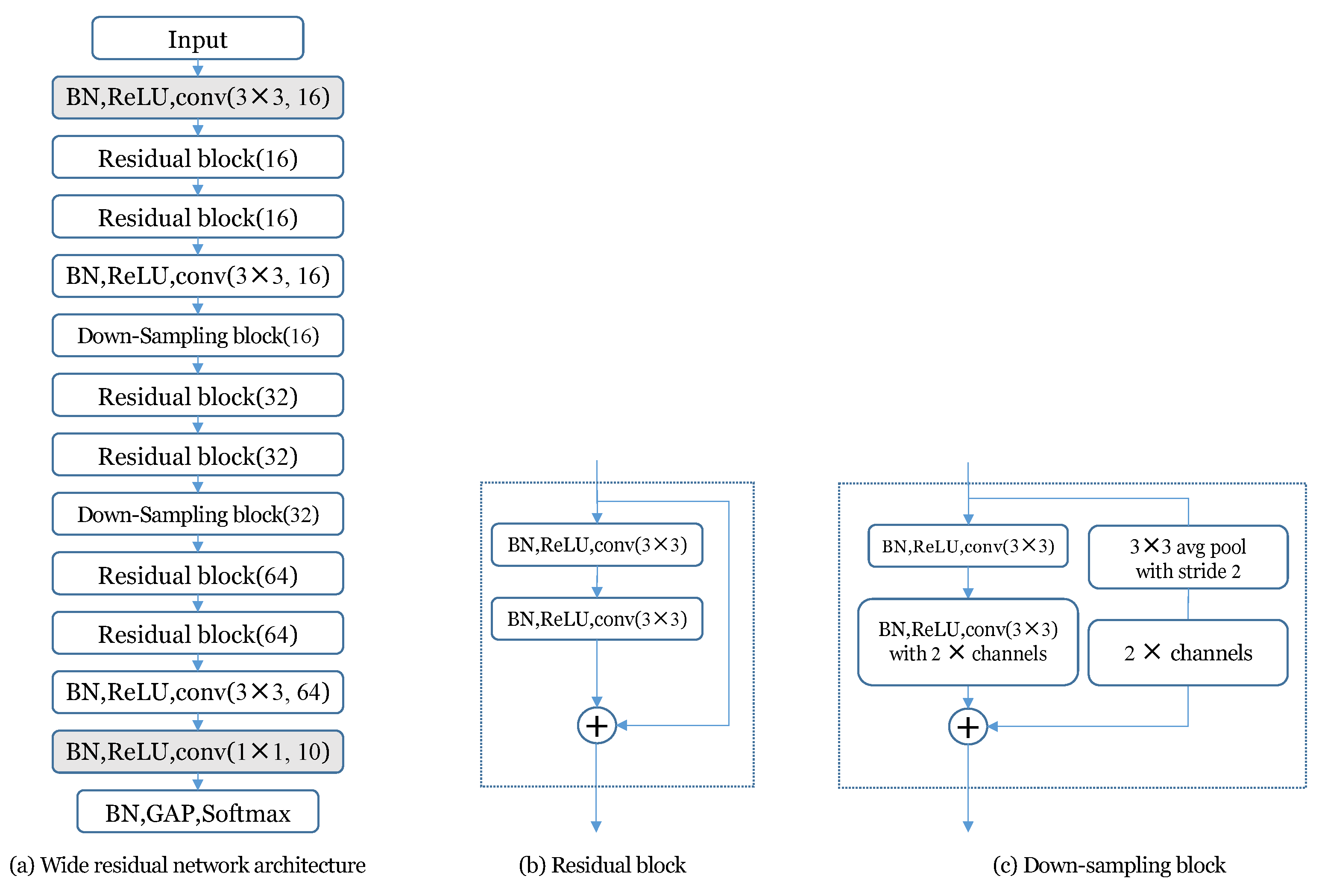
| Low Frequency (1st–128th bins) | High Frequency (129th–256th bins) |
|---|---|
| CNN (1 × 1, 32) | CNN (1 × 1, 32) |
| Batch Normalization ReLU Activation | Batch Normalization ReLU Activation |
| Residual Block (32) × 2 | Residual Block (32) × 2 |
| Max Pooling (2 × 2) | Max Pooling (2 × 2) |
| Residual Block (64) × 2 | Residual Block (64) × 2 |
| Max Pooling (2 × 2) | Max Pooling (2 × 2) |
| Residual Block (64) × 2 | Residual Block (64) × 2 |
| CNN (1 × 1, 32) | CNN (1 × 1, 32) |
| CNN (1 × 1, 64) | CNN (1 × 1, 64) |
| Batch Normalization | Batch Normalization |
| Concatenation along freq. axis | |
| CNN (1 × 1, 10) | |
| Global Average Pooling Softmax Activation | |
| Model | Log Loss | Macro-Averaged F-Score | Model Size |
|---|---|---|---|
| Vanilla | 1.052 | 65.79% | 125.8 KB |
| Conventional Temporal Ensembling | 1.042 | 62.26% | 125.8 KB |
| Conventional Mean-Teacher | 1.069 | 66.47% | 125.8 KB |
| Temporal Ensembling w/Unit Step | 1.023 | 65.93% | 125.8 KB |
| Modified Mean-Teacher (Proposed) | 1.009 | 67.12% | 125.8 KB |
| Method | Log Loss | Macro-Averaged F-Score | Model Size |
|---|---|---|---|
| DCASE 2021 Task 1A Baseline (in [20]) | 1.47 | 47.7% | 90.3 KB |
| Vanilla model (ours) | 1.05 | 65.8% | 125.8 KB |
| Mean-Teacher model (ours) | 1.01 | 67.1% | 125.8 KB |
| Liu’s model (in [21]) | 0.92 | 68.0% | 42.5 KB |
| Liu’s model + Feature Reuse (in [21]) | 0.91 | 68.2% | 106.7 KB |
| Koutini’s model (in [14]) | 0.89 | 69.4% | 127.7 KB |
| Koutini’s model + Domain Adaptation (in [14]) | 0.88 | 69.5% | 127.5 KB |
| Heo’s model (in [33]) | - | 68.5% | 124.1 KB |
| Heo’s model + Knowledge Distillation (in [33]) | - | 70.5% | 124.1 KB |
| Consistency Weight | Log Loss | Macro-Averaged F-Score [%] |
|---|---|---|
| 1.045 | 65.66% | |
| 1.009 | 67.12% | |
| 1.013 | 66.07% | |
| 1.019 | 66.03% |
| Start Epoch | Log Loss | Macro-Averaged F-Score |
|---|---|---|
| 1.060 | 63.55% | |
| 1.048 | 64.32% | |
| 1.049 | 65.53% | |
| 1.040 | 66.04% | |
| 1.022 | 66.20% | |
| 1.009 | 67.12% | |
| 1.027 | 65.70% | |
| Ramp-up for 260 epochs | 1.045 | 65.82% |
| SNR | Log Loss | Macro-Averaged F-Score |
|---|---|---|
| Without noise | 1.041 | 65.97% |
| 70 dB | 1.041 | 66.03% |
| 60 dB | 1.009 | 67.12% |
| 50 dB | 1.028 | 66.39% |
| Method | Log Loss | Macro-Averaged F-Score |
|---|---|---|
| Without noise | 1.041 | 65.97% |
| Both models, throughout training | 1.045 | 66.30% |
| Student model only, throughout training | 1.025 | 66.92% |
| Student model only, | 1.009 | 67.12% |
| Model | Log Loss | Macro-Averaged F-Score | Model Size |
|---|---|---|---|
| Vanilla | 1.035 | 65.44% | 43.6 KB |
| Proposed Mean-Teacher with | 1.027 | 66.15% | 43.6 KB |
| Proposed Mean-Teacher with | 1.012 | 67.05% | 43.6 KB |
| Proposed Mean-Teacher with | 1.004 | 67.49% | 43.6 KB |
| Proposed Mean-Teacher with | 1.035 | 66.55% | 43.6 KB |
Publisher’s Note: MDPI stays neutral with regard to jurisdictional claims in published maps and institutional affiliations. |
© 2021 by the authors. Licensee MDPI, Basel, Switzerland. This article is an open access article distributed under the terms and conditions of the Creative Commons Attribution (CC BY) license (https://creativecommons.org/licenses/by/4.0/).
Share and Cite
Lee, S.; Kim, M.; Shin, S.; Baek, S.; Park, S.; Jeong, Y. Ensemble-Guided Model for Performance Enhancement in Model-Complexity-Limited Acoustic Scene Classification. Appl. Sci. 2022, 12, 44. https://doi.org/10.3390/app12010044
Lee S, Kim M, Shin S, Baek S, Park S, Jeong Y. Ensemble-Guided Model for Performance Enhancement in Model-Complexity-Limited Acoustic Scene Classification. Applied Sciences. 2022; 12(1):44. https://doi.org/10.3390/app12010044
Chicago/Turabian StyleLee, Seokjin, Minhan Kim, Seunghyeon Shin, Seungjae Baek, Sooyoung Park, and Youngho Jeong. 2022. "Ensemble-Guided Model for Performance Enhancement in Model-Complexity-Limited Acoustic Scene Classification" Applied Sciences 12, no. 1: 44. https://doi.org/10.3390/app12010044