In this section, we conduct experimental studies of the proposed approach on five datasets.
4.1. Datasets
The description of each dataset is given as follows.
Synthetic dataset [
15]: The synthetic two-dimensional dataset contains three classes. Each class follows the Gaussian distribution. The dataset contains 750 samples, and there are 250, 300 and 200 samples in each class, respectively.
Forest [
46]: The Forest dataset is from UCI Machine Learning Repository. This dataset contains training and testing data from a remote sensing study which mapped different forest types based on their spectral characteristics at visible-to-near infrared wavelengths of four types (“s”-“Sugi” forest, “h”-“Hinoki” forest, “d”-“Mixed deciduous” forest, “o”-“Other” non-forest land). The original data contains 27 attributes, of which 1–9 are numerical spectral properties, 10–27 are non-numerical attributes. We only took the first nine columns of numerical properties for the experiment followed by merging the training set and the test set in the original data, a total of 523 samples as a 523 × 9 array.
Pendigits [
47]: The dataset which is a digit database by collecting 250 samples from 44 writers stored in a 10,992 × 16 array. It is also from UCI Machine Learning Repository.
MNIST [
48]: The MNIST database contains a total of 70,000 examples of handwritten digits of size 28 × 28 pixels. It is a subset of a larger set available from NIST. The digits have been size-normalized and centered in a fixed-size image.
MIT face [
49]: This dataset from MIT contains synthetic face images of 10 subjects with 324 images per item. These synthetic images were rendered from 3D head models and stored as a 64 × 64 size figure. The final dataset is stored as an array of 3240 × 4096, containing ten different categories for a different subject.
Table 1 shows the summarized characteristics of five datasets involved in the experiment.
4.2. Initialization Method
The dataset needs to be preprocessed before starting the classification experiment. To ensure the rationality of the dataset segmentation, the data of each category is firstly extracted proportionally and then spliced together as the training set. Finally, we shuffle the samples in the training set, and the remaining data is regraded as the test set.
For the initialization of the parameter P, we try a variety of methods.
The first one is to perform K-means on each type of training set and get the clustering centers as the initial prototypes.
The second way is to get the clustering centers by K-means in the entire training set to get the initial prototypes.
The third way is to select samples in each category as prototypes randomly.
The last way is to take the average of each category of data as initialization.
Along with our paper, we assume the number of clusters in initialization is equal to the number of prototypes. The first three methods take a proportional number of prototypes M to the number of categories K. Notice that we define K is the number of categories, and K is not related to K-means in our scenario. The final method takes the mass centers of the samples from each class as the prototypes, and it assumes the number of prototypes equal to the number of categories. In the experimental section, we will compare these four initialization methods to investigate the effects of different prototype initialization methods.
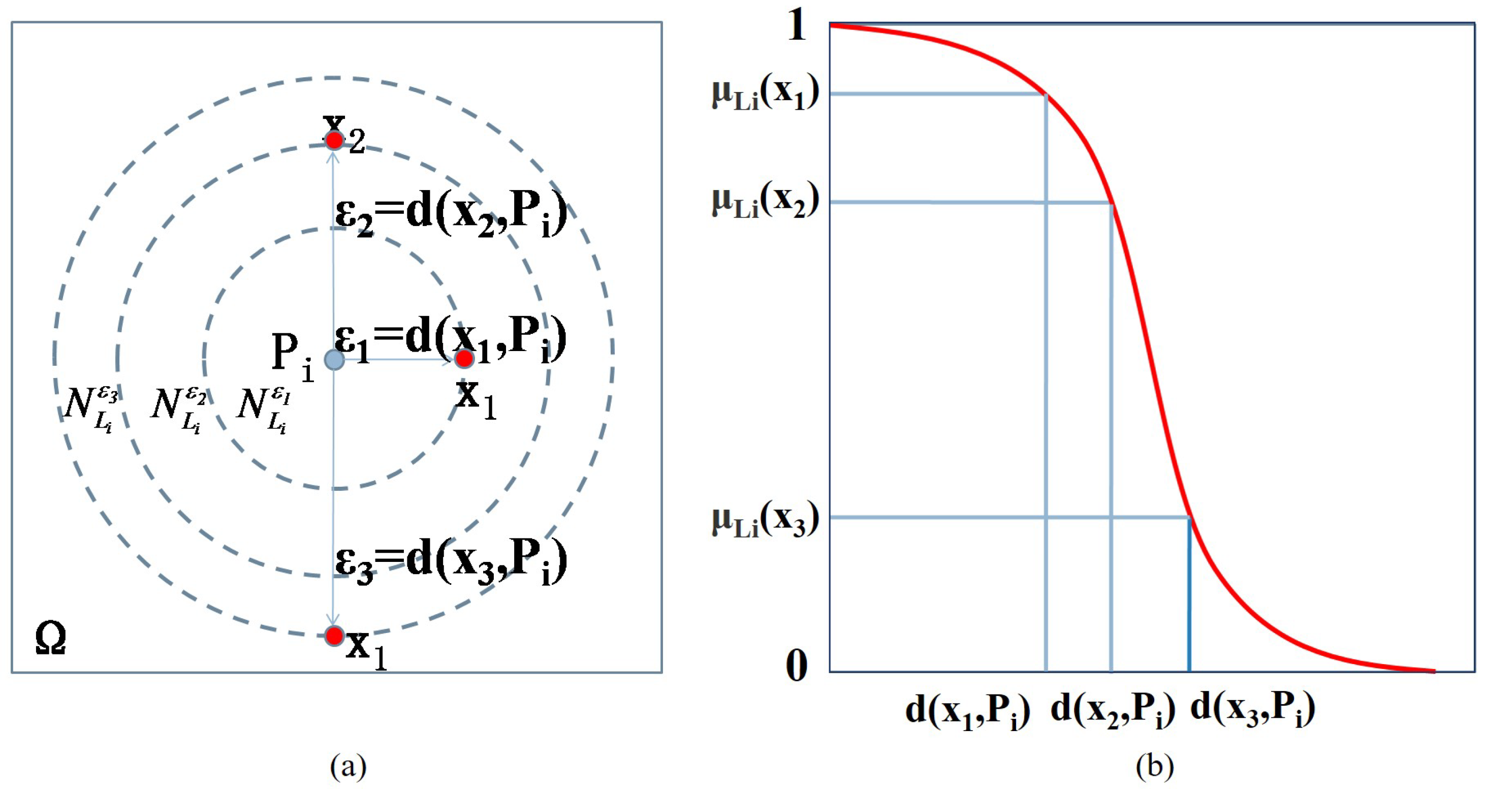
For the parameter , as a parameter for controlling the bell-shaped distribution width, experiments show that the initialization of will affect the convergence speed and the classification result of the algorithm. Empirically we discovered that a better classification result can be obtained when the value of is one-third of the average distance between training set samples and the corresponding prototype. However, no additional theoretical support for this phenomenon has been discovered. We will leave it for future work.
4.3. Experimental Results
Table 2 shows the changes of classification accuracy under different training set scales. We repeat the experiment 100 times to obtain the mean and standard deviation of the classification results, considering the randomness of the dataset segmentation and differences in initializing parameters. In this experiment, we use the second initialization method of
P. In particular, we use K-means to initialize one prototype in each class and then combine them together as the prototype initialization. As an initialization for
, we take one-third of the average distances between the samples of each category and the prototypes. From the experimental results, we can see that our method is robust. Even in the case of a small amount of data (only 10%), we can get an acceptable classification result.
For the initialization of the prototype, we can limit the initialization method and the number of initial prototypes. In the following two experiments, 30% (3290 samples) of the Pendigits dataset were used as the training set and the rest as the test set (7702 samples).
Table 3 shows the difference in classification results for different numbers of prototypes. We initialize one to four prototypes in each category (a total of 10 categories) by K-means, so the number of prototypes ranges from 10 to 40 in the prototype initialization. We also set
as one-third of the average distance that the samples of each category to the prototypes. We also repeated the experiment 10 times to obtain the mean and standard deviation of the classification results, taking into account the randomness of dataset segmentation and differences in initializing parameters. The experimental results are consistent with the above analysis. The classification effect will improve as the number of prototypes increases. As a result, as the number of prototypes grows, so the computational complexity also increases. At the same time, if there were too many prototypes, most fuzzy semantic cell will become too small and redundant. As a result, we must select the appropriate number of prototypes to strike a balance between computational efficiency and classification effect.
In the following experiment, we conducted a controlled trial in four ways as described in
Section 4.2 to show the classification accuracy under different initialization methods of prototypes on Pendigits dataset as shown in
Table 4. We used ten prototypes (
), and the initialization method of
is the same as before. The experiment is repeated six times. The experimental results show that the training accuracy decays slightly since more samples are difficult to fit. However, the testing accuracy increases substantially as the model learns more about the training distribution. Despite the objective function being a non-convex problem, the classification effect is nearly stable across the different prototype initialization methods. When prototypes are initialized by category, the results are consistent after repeated experiments, and the standard deviation is low. When the prototypes are initialized with a global method, the overall classification accuracy is not significantly worse, though the result is slightly different and the standard deviation is relatively larger. In the last prototype initialization with 0.3 and 0.5 as the training ratio, the average training accuracy is slightly lower than the testing accuracy. However, when considering the deviation, such difference is not significant. We attribute this phenomenon to randomness.
Using Adam [
17] is based on the following empirical findings. The learning problem of our method is an unconstrained non-convex optimization, and the loss is estimated within batches of samples. It has been shown Adam converges faster than other first-order optimization methods do [
17], like SGD and RMSprop [
50]. For second-order optimization methods, Newton and Quasi-Newton require expensive computation and memory cost. Besides, L-BFGS is an efficient Quasi-Newton approximation. We conduct experiments on SGD, RMSprop and L-BFGS. We use the fourth initialization method of prototypes and compares the test accuracy in
Table 5. The L-BFGS introduce instability when the ratio is 0.1. The performances of other methods are worse than Adam in this scenario. Evolutionary optimization and particle swarm optimization are also used in related works [
26,
27], but we believe numerical optimization methods are more reproducible.
In the final experiment, we compared the differences between the proposed method and the six conventional classification methods. We conduct this experiment with packages in scikit-learn [
51]. SVM uses the polynomial kernel function, and AdaBoost’s learning rate is set to
. The Neural Network is a multi-layer perceptron model of two hidden layers, which have five and two neurons, respectively. The nonlinear activation is ReLU, and the out neurons are softmaxed to give a probability distribution. To optimize the model, a cross-entropy loss and an L-BFGS optimizer are used. Other settings are the default. We test typical classification methods (DecisionTree, NaiveBayes, KNN, SVM, AdaBoost, Neural Network) in classification accuracy for five different datasets. For each dataset, we select 10% as the training set and the remaining 90% as the test set to compare the classification effects in the case of a small size of the training set. Because fewer samples are employed for training, most algorithms can achieve outstanding performances on the training set, but algorithms perform variedly on the test set. The classification accuracy on the test set is shown in
Table 6.
From the results in
Table 6, we can conclude that seven algorithms have similar performance on the synthetic datasets. When the sample size used for the training is relatively large, the neural network algorithm has the best consequences, such as in handwritten datasets Pendigits and MNIST. However, when the number of training samples are small, the neural network algorithm stability rapidly declines. Not only does the classification effect deteriorate, but it also fluctuates dramatically (high standard deviation) in the Forest and MIT face datasets. In contrast, regardless of the amount of data, the algorithm proposed in this paper produces a stable output. Moreover, we also found that the KNN algorithm also has outstanding performance on different datasets. However, a better performance of KNN is reached when the parameter of neighborhood is manually chosen.Accordingly, in our algorithm, the same parameter initialization method is utilized for all datasets, and a general classification algorithm is obtained without further human intervention. In this experiment, we use K-means (K = 3) in each category as the prototype initialization and take one-third of average distances that the samples of each class to the prototypes as corresponding
initialization. The Naive Bayes algorithm is more sensitive to datasets and has diverse experimental results for different datasets. For example, it has a better performance on Forest datasets but lags behind other methods on MIT face datasets. This shows that the NaiveBayes algorithm does not have a strong generalization ability. The performance of the SVM algorithm on each dataset is neither remarkable nor bad. As for the DecisionTree algorithm and AdaBoost algorithm, the performance lags behind other algorithms when only 10% of the data is used as a training set. In general, the method proposed in this paper has strong competitiveness both in terms of classification effect, robustness and generalization ability.
Further experiments show that the Euclidean distance measurement method is not applicable in high-dimensional data spaces. However, after dimension reduction, the data can produce notable experimental results. As a result, the classification results for the high-dimensional data in this experiment are based on the data after dimension reduction.
In most of our experiments, we repeat six times. The reason for this is to reduce estimation error. We find most existing works repeat experiments three times to get the average and standard deviation of performances for comparison. Suppose the standard variance of the ground-truth performance as a random variable is , so the standard variance of an average of three repeats is . As the mean is an unbiased estimation of the expectation, the standard variance is equivalent to the estimation error. The three-time repeat is an acceptable balance between computational cost and estimation accuracy. As our method is trained on a small number of samples, we are able to repeat six times to get a more precise estimation, with a standard variance of .


