Multi-Objective Optimization of CO₂ Sequestration in Heterogeneous Saline Aquifers under Geological Uncertainty

Abstract

This paper presents a Pareto-based multi-objective optimization for operating CO₂ sequestration with a multi-well system under geological uncertainty; the optimal well allocation, i.e., the optimal allocation of CO₂ rates at injection wells, is obtained when there is minimum operation pressure as well as maximum sequestration efficiency. The distance-based generalized sensitivity analysis evaluates the influence of geological uncertainty on the amount of CO₂ sequestration through four injection wells at 3D heterogeneous saline aquifers. The spatial properties significantly influencing the trapping volume, in descending order of influence, are mean sandstone porosity, mean sandstone permeability, shale volume ratio, and the Dykstra–Parsons coefficient of permeability. This confirms the importance of storable capacity and heterogeneity in quantitatively analyzing the trapping mechanisms. Multi-objective optimization involves the use of two aquifer models relevant to heterogeneity; one is highly heterogeneous and the other is less so. The optimal well allocations converge to non-dominated solutions and result in a large injection through one specific well, which generates the wide spread of a highly mobile CO₂ plume. As the aquifer becomes heterogeneous with a large shale volume and a high Dykstra–Parsons coefficient, the trapping performances of the combined structural and residual sequestration plateau relatively early. The results discuss the effects of spatial heterogeneity on achieving CO₂ geological storage, and they provide an operation strategy including multi-objective optimization.

1. Introduction

A challenging problem in engineering analytics has been the existence of many objectives. Multi-objective optimization attempts to find the optimal trade-offs that are most acceptable to the decision maker among all objective functions [1,2,3]. The Pareto front, i.e., a set of Pareto solutions, illustrates the trade-offs for which algorithms should secure solution diversity as well as make comparative evaluations among the potential solutions [4,5,6,7,8]. Evolutionary multi-objective optimization (EMO) algorithms, e.g., the non-dominated sorting genetic algorithm (NSGA; NSGA-II; NSGA-III), strength Pareto evolutionary algorithm (SPEA; SPEA-II), Pareto envelope-based selection algorithm (PESA; PESA-II), and multi-objective evolutionary algorithm based on decomposition (MOEA/D), have continuously improved fitness assignment and diversity control [1,2,3,4,5,6,7,8,9,10]. NSGA is a well-known scheme designed to preserve non-dominated points in objective space that also has a wide solution-searching capability with a genetic algorithm. Its strength is that it can provide non-dominated trade-offs in the comparison of objective functions, while its weaknesses are the fact that it requires a large amount of computing power and its decreasing convergence with an increasing number of objective functions, i.e., ‘the curse of dimensionality’ [5,6,7,8,9,10].

Geological uncertainty limits quantitative analyses of subsurface flow [11,12,13,14]. The input uncertainties in geo-modeling are non-linearly interacted; some are heterogeneous (e.g., porosity, permeability, and lithology) while others are functional (e.g., relative permeability, solubility, and capillary pressure) or scenario-based (e.g., the depositional system) [13,14,15,16,17]. The flow responses are spatiotemporal. Sensitivity measures the relationship between the inputs and the responses and, thus, denotes some influential parameters that significantly affect the responses. The stochastic features between the inputs and the responses do not result in the emergence of a certain parameter as a significant factor but instead require multi-way parameter interactions. The distance-based generalized sensitivity analysis (DGSA) has been successfully used to evaluate the significance of scale-variant properties in heterogeneous geo-models [10,15,16,17,18,19]. Fenwick et al. [15] quantified the interaction of asymmetric parameters such as residual oil saturation, maximum water relative permeability, and training images. Park et al. [16] analyzed spatial uncertainty using kernel principal components and self-organizing maps.

CO₂ sequestration into deep saline aquifers, e.g., around 1 km below ground level, is known to have enormous storage potential, but little is known about its geological characterization and project experiences compared to those of depleted oil or gas reservoirs. The significant uncertainties can be categorized into capacity, injectivity, and containment: the capacity determines the storable amount, the injectivity estimates the possible injection rates, and the containment evaluates the risks of leakage [20,21,22,23,24]. Bachu [20] explained the importance of the hydrodynamic and buoyancy forces needed for the CO₂ plume to propagate into the homogeneous saline formation. Kumar et al. [21] discussed the key factors related to the rock and fluid properties, reservoir conditions, and injection strategy as storage mechanisms (structural, residual, solubility, and mineral trapping) in saline aquifers; these include reservoir heterogeneity, depth, permeability, pressure, and temperature. Along with these geological properties, the injection pressure is one of the crucial operating parameters depending on the containment and the security. One reason for this is the well injectivity—defined as the CO₂ injection mass rate per unit pressure differential—which determines the total CO₂ amount injected into the geological formation. On the other hand, the safety constraint is that the injection pressure (the bottom hole pressure; BHP) should be lower than the formation fracture pressure so as to prevent CO₂ leakage or fast movement without trapping [25,26,27,28,29,30]. When CO₂ is injected into a porous medium using multi-injectors, the well allocation, i.e., the allocation of CO₂ amount at each injector, worsens the problem; the well allocation at the heterogeneous aquifers would involve a lot of scenarios, so the optimization process could be subject to the issue of convergence [31,32,33,34,35,36,37,38,39,40,41,42].

This study intends to search for trade-offs between cost and containment efficiency as a multi-objective problem for CO₂ sequestration into heterogeneous saline aquifers; the cost is related to the CO₂ injection pressure used to operate the facilities, while the containment efficiency involves storing as much CO₂ as possible while considering the amount of CO₂ injected. Well allocation constructs variable spaces, while two objective functions (the injection pressure and the sequestration efficiency) constitute the posterior domain. The uncertainty assessment of spatial properties should be made prior to multi-objective optimization because the subsurface aquifers are heterogeneous in nature and their properties are uncertain.

2. Materials and Methods

2.1. 3D Heterogeneous Aquifer Models and Simulation Conditions

A total of 1024 heterogeneous aquifers are constructed geostatistically under spatial uncertainty of permeability and porosity. The spatial distribution of these properties is modeled using Petrel (Schlumberger, Houston, TX, USA). Three dimensional unstructured grid systems are generated to demonstrate both the upward CO₂ movement and the horizontal flow. Total number of unstructured grids is 22,230 (= 38 × 45 × 13). The saline aquifer size is (x, y, z) = (6310 m, 7076 m, 250 m). It is assumed that the impermeable cap rock is located at 840 m true vertical depth. Dykstra–Parsons coefficients ($v_{DP}$) measure permeability heterogeneity between 0 and 1 (Equation (1)).

$$v_{DP}=\frac{k_{0.5}-k_{0.841}}{k_{0.5}}$$

(1)

In Equation (1), $k_{0.5}$ is the mean value and $k_{0.841}$ is the value placed at one standard deviation plus the mean [43,44]. $v_{\mathrm{DP}}=0$ means that the medium is homogeneous. The higher the Dykstra–Parsons coefficient is, the more heterogeneous the medium is. The ratio of vertical to horizontal permeability is 0.1 and the permeabilities are isotropic horizontally (x and y directions).

Table 1. Spatial properties to construct the heterogeneous aquifer models.

Property	Abbreviation	Value Range
1 Mean permeability of sandstone 2 (millidarcy)	PermSand	300~450
Mean porosity of sandstone (unitless)	PoroSand	0.22~0.28
3 Std of permeability (sandstone; millidarcy)	StdPerm	12.5~50
Std of porosity (sandstone; unitless)	StdPoro	0.005~0.02
Shale volume ratio (%)	SVR	2~20
Dykstra–Parsons coefficient (unitless)	VDP	0.1896~0.9185

¹ The horizontal permeabilities for each geo-model are arithmetic averaged; ² 1 millidarcy = 9.869 × 10⁻¹⁰ m²; ³ ‘Std’ stands for the standard deviation.

summarizes the input ranges of the spatial properties for constructing 3D heterogeneous aquifers. The stochastic realizations, i.e., geostatistical property modeling, are carried out with the inputs randomly selected (Table 1). The heterogeneous geo-models are made with massive sandstone intercalated with almost impermeable shale (Figure 1). Shale is placed at the bottom of aquifer and interbedded in sandstone; the former is to prevent leakage at the early time and the latter is to demonstrate the realistic heterogeneous aquifers. The shale volume ratio is defined as the ratio of shale volume to the rock volume and represents the effects of shale layers; this is selected between 2 and 20%. The shale porosities (ranging from 0.1 and 0.15) are smaller than those of sandstone. The shale permeabilities (ranging from 0.05 and 0.5 millidarcy) represent almost impermeable barriers The standard deviations of shale permeability and porosity are negligible compared to sandstone. The end point of relative permeability at the irreducible water saturation (= 0.1) is 0.85, while that at the irreducible CO₂ saturation (= 0.2) sets as 0.2.

Figure 1 illustrates an example of heterogeneous aquifer models with four injectors (namely, I1, I2, I3 and I4). Figure 1a depicts the spatial distribution of permeability and Figure 1b describes that of porosity. The injection wells are installed to evenly divide the entire aquifer; (x, y) grid positions are as follows, I1 = (10, 12), I2 = (28, 12), I3 = (10, 34), and I4 = (28, 34). The perforation zone in z direction is from 1032.3 m to 1051.53 m, the lower part of the aquifer. The wells are partially perforated, over the less permeable basement rock (the shale layer), to demonstrate the upward movement of CO₂ plume. MRST (MATLAB Reservoir Simulation Toolbox) is used to simulate CO₂ sequestration in saline aquifers [44,45]. It provides various trapping volumes: a volume of combined structural and residual trapping, a volume of residual trapping, a volume of residual trapping with plume, a volume of structural trapping, and a volume of movable plume, respectively. CO₂ properties are assessed using CO2 Lab module in MRST [44]. The reference pore-pressure is 120 bar and the temperature is 45 degrees Celsius at the top of the aquifer (840 m depth) where the formation fracture pressure is 150 bar. CO₂ viscosity is set as 0.051 centipoise (1 centipoise = 10⁻³ Pa∙s) and its density is 675.324 kg/m³ at the given reference pressure and temperature. Brine density is 975.86 kg/m³.

Figure 1. An example of heterogeneous aquifer models with four injection wells. The distributed properties are (a) absolute permeability (horizontal permeability) and (b) porosity. Dykstra–Parsons coefficient = 0.752; shale volume ratio = 8%; the mean porosity (including sandstone and shale) = 0.226; the mean permeability (including sandstone and shale) = 301 millidarcy.

Figure 1. An example of heterogeneous aquifer models with four injection wells. The distributed properties are (a) absolute permeability (horizontal permeability) and (b) porosity. Dykstra–Parsons coefficient = 0.752; shale volume ratio = 8%; the mean porosity (including sandstone and shale) = 0.226; the mean permeability (including sandstone and shale) = 301 millidarcy.

2.2. DGSA for Evaluating the Significance of Spatial Properties

DGSA, based on regionalized sensitivity analysis, defines the cumulative density functions (CDF) distance [15,16]. The distance reflects variational properties of the responses or the dimensionality-reduced responses [16]. After classifying of the output response with a clustering scheme, the class can generate CDF and the distance can be defined as L1 norm between two CDFs (Equation (2)).

$${\widehat{d}}_{c,i}=d_{L1}\left(\widehat{G}\left(p_i\right), \widehat{G}\left(p_i|c\right)\right), c=1,2,\cdots , C; i=1,2,\cdots ,m$$

(2)

In Equation (2), ${\widehat{d}}_{c,i}$ is the CDF distance (L1 norm distance, $d_{L1}$) between the input CDF for parameter $p_i$ and the CDF of the parameter in the class, c. $\widehat{G}\left(p_i\right)$ is an empirical distribution function from sampling. $\widehat{G}\left(p_i|c\right)$ is a class-conditioned empirical distribution function after classification. C is the number of class that the modeler pre-assigned and m is the number of parameters. The measure of sensitivity is standardized by the resampling quantile of the distance. DGSA introduced multidimensional scaling, characterized the population and the clusters using CDF, and tested the asymmetric interactions of spatiotemporal parameters using the distance between CDFs (L1 norm) [15,16,17,18,19].

2.3. NSGA-II for Multi-Objective Optimization Calibrating Well Allocations

Pareto optimality, i.e., the trade-off solutions, is the non-domination where no solution can be improved with respect to any objective without worsening at least another objective [4,5,8]. Multi-objective evolutionary algorithm searches the trade-offs that would give a vector of decision variables for all the objective functions under any given constraints (Equation (3)).

$$f\left(X\right)={\left[f_1\left(X\right), f_2\left(X\right), \cdots ,f_n\left(X\right)\right]}^T$$

(3)

In Equation (3), $f\left(X\right)$ is an objective function with the vector (X) of decision variables, e.g., well allocation in this study, and the subscript n is the number of objective functions. NSGA-II algorithm consists of competing individuals with a genetic algorithm, non-dominated sorting, and crowding distance [5,7,8,9,10]. The genetic algorithm-based operations, e.g., crossover and mutation, form the offspring and then the individuals in the mixture of parent and offspring population are competing with non-dominated sorting and the crowding distance. The non-dominated sorting strategy of NSGA-II proceeds by comparing each individual one by one, and when a non-dominated front is found, it is temporarily stored, and then the next non-dominated front is searched. This non-dominated sorting continues until all individuals are ranked [1,5] (Figure 2). The solutions can evolve to the direction of the real Pareto optimization set, as a larger probability is assigned to the individuals in the lowest dominant level in order to select the superior individuals into the next generation of the population.

To maintain the solution diversity, the crowding distance calculates the congestion degree of each individual and other individuals [7,8,9] (Figure 2). Equation (4) defines the $k$–th individual’s crowding distance (${\delta }_k$).

$${\delta }_k=\frac{1}{n}{\displaystyle \sum }_{i=1}^n\frac{f_i\left(k+1\right)-f_i\left(k-1\right)}{f_i^{max}-f_i^{min}}$$

(4)

In Equation (4), $f_i\left(k+1\right)$ and $f_i\left(k-1\right)$ indicate $i$-th objective function values for $\left(k+1\right)$-th and $\left(k-1\right)$-th individual, respectively. $f_i^{max}$ is the maximum value, and $f_i^{min}$ is the minimum for $i$-th objective function. By selecting the individuals with lower crowding distance value in the same dominant level, the evenness and diversity of the evolutional population can be guaranteed [9,10]. Pareto optimality can be obtained by reaching convergence conditions, or by repeating the process up to the maximum number of evolutions, and, thus, multi-objective optimization is costly because of enormous computational simulations.

3. Results and Discussion

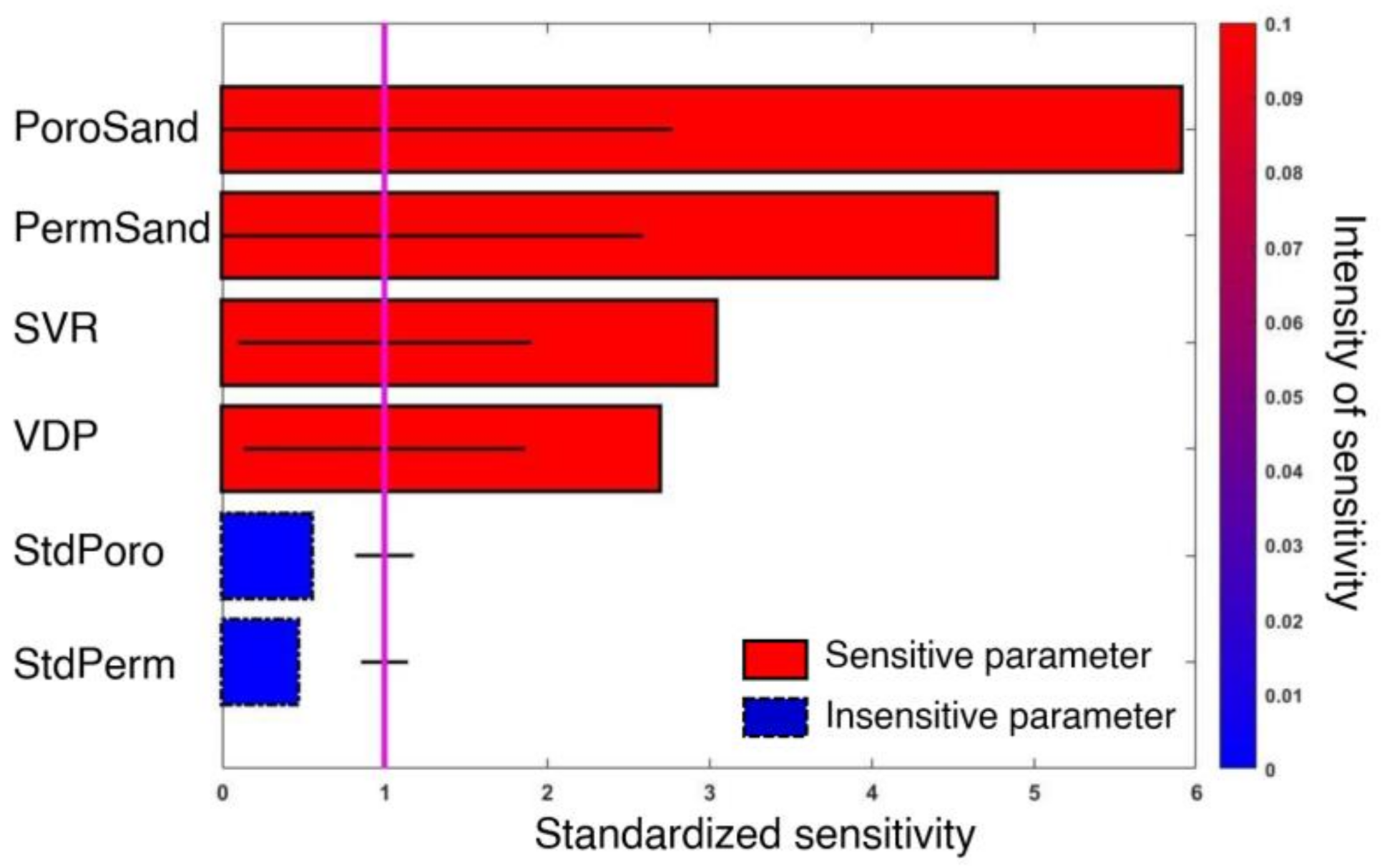
3.1. Spatial Properties Influencing CO₂ Trapping

DGSA parameters are assigned as follows: k-medoid clustering, with six clusters, classifies 1024 aquifer models and the resampling quantile of distance is 0.95. A response for DGSA is the trapping volume of combined structural and residual trapping, representing relatively permanent and safe sequestration. The trapping amount is a cumulative volume during 200 years from the first injection. Six uncertain parameters (C = 6 in Equation (2)) are mean sandstone porosity, mean sandstone permeability, standard deviation of sandstone porosity, standard deviation of sandstone permeability, shale volume ratio, and Dykstra–Parsons coefficient, respectively (m = 6 in Equation (2); Table 1). To remove the effects of well allocation, a constant injection rate, 4000 m³/day for each injector is assumed. Total injection rate per day is 16,000 m³/day because four injectors are placed (Figure 1a). CO₂ is injected continuously for 30 years and the trapping trend is monitored for 200 years, i.e., an additional 170 years from the end of CO₂ injection.

Figure 3 depicts the result of DGSA with spatial parameters; the sensitive parameters are the mean porosity of sandstone (PoroSand), mean permeability of sandstone (PermSand), shale volume ratio (SVR), and Dykstra–Parsons coefficient (VDP) in each row. The vertical line (the standardized sensitivity = 1; the significant level) indicates whether the parameter influences the response. The larger standardized sensitivity means more influence. The sensitive parameters support the importance of heterogeneity and aquifer properties on CO₂ trapping: PoroSand determines the capacity size, PermSand affects CO₂ mobility, SVR and VDP represent the effects of the shale barrier on storage and transport, respectively. The trapping amounts significantly depend on the pore volume of sandstone. The other parameters over the significant level are closely related to CO₂ flow. With increasing SVR and VDP, shale is likely to obstruct CO₂ flow. However, this would be a subject of discussion as to whether the large amount of shale always has a positive effect on the trapping volume. The asymmetric parameter interactions can make this debate more complicated as a parameter can simultaneously influence the different responses. If the operating conditions are included, deriving a reasonable conclusion would become a conundrum.

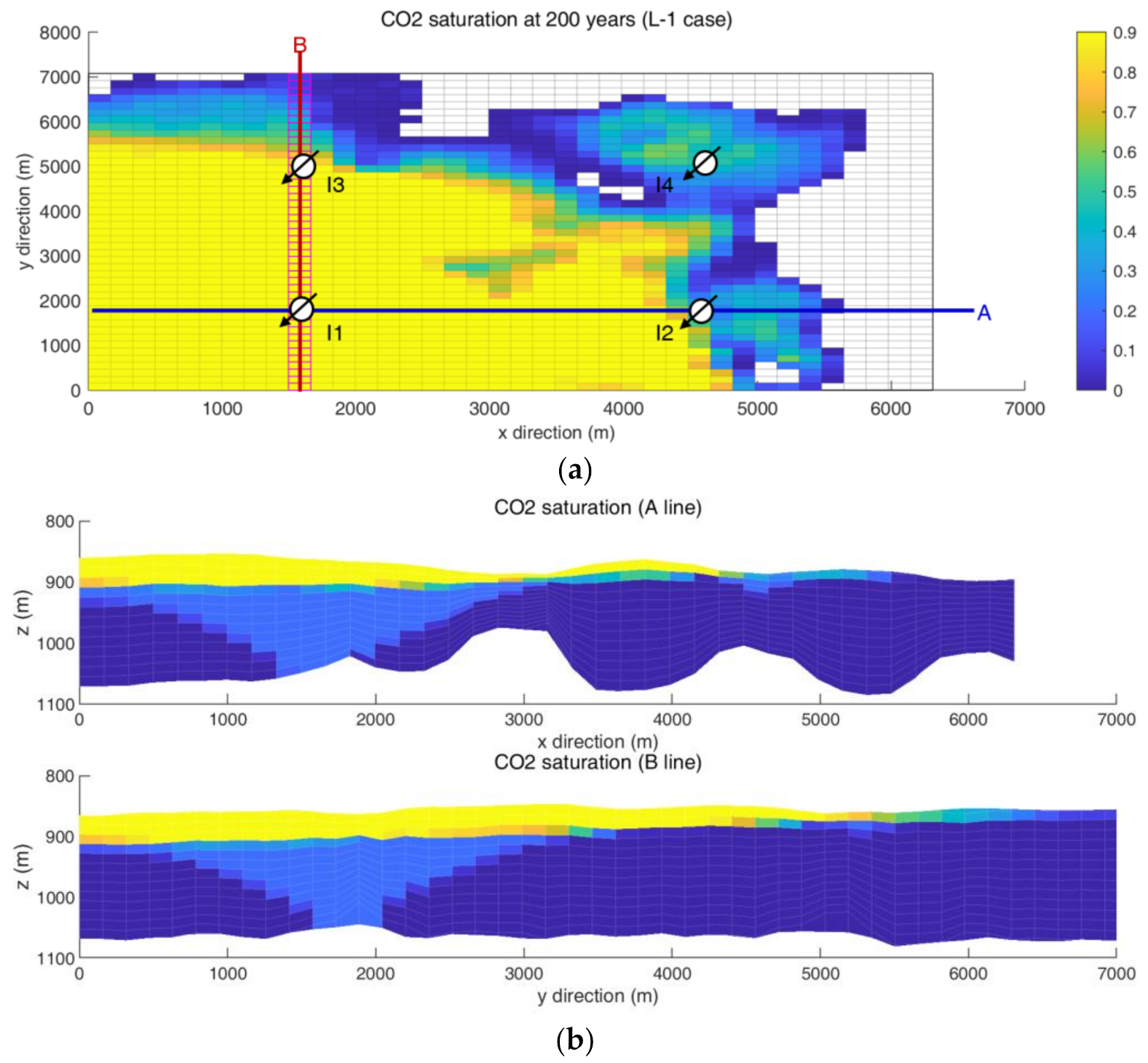
3.2. Multi-Objective Optimization with Well Allocations

Multi-objective optimization requires a lot of simulation runs and, thereby, this work selects two different aquifers based on the DGDA result (

Table 2. Two heterogeneous aquifers for multi-objective problem with well allocation.

Property (Abbreviation) 1	L Aquifer	H Aquifer
PoroSand	0.274	0.220
PermSand	301.5	448.7
SVR	2	20
VDP	0.3488	0.9169
StdPoro	0.012	0.012
StdPerm	14.0	30.7

¹ Table 1 defines the abbreviations.

; Figure 4); one is the less heterogeneous (L aquifer; less heterogeneous relevant to the small value of Dykstra–Parsons coefficient) and the other is highly heterogeneous (H aquifer; the high heterogeneity). Figure 4 demonstrates spatial distributions of the key properties influencing the trapping amount: Figure 4a,b show permeability and porosity of L aquifer, while Figure 4c,d illustrate those of H aquifer. Upon comparison of the two aquifers, L aquifer is capable of storing more CO₂ and induces slow fluid transport through sandstones (because L aquifer has the smaller sandstone permeability and the larger sandstone porosity; refer to Table 2).

On the other hand, H aquifer is more ambiguous in terms of fluid transport. It has a large portion of shale formations (negative to the continuity of fluid flow) but more permeable sandstones (favorable to a transporting velocity). The former, i.e., shale beds, would be advantageous for long-term CO₂ geological storage, while a drawback would be having to maintain the lower injection pressure since shale can increase the operating cost to inject CO₂ continuously. The more permeable sandstone has double-sidedness as well; the higher transmissivity contributes towards the spread of supercritical CO₂ widely, to occupy additional pore spaces, but can increase the risk of leakage. Therefore, this paper selects H aquifer with overall mean permeability including both sandstone and shale similar to L aquifer model, notwithstanding that H aquifer is more heterogeneous; the entire mean permeability of L aquifer is 227 millidarcy and it is 256 millidarcy for H aquifer, which occupies less permeable shales and reduces the difference in PermSand from 147.2 millidarcy (= 448.7–301.5) to 29 millidarcy (= 256–227). Shales distribute sparsely, are intercalated with the massive sandstone, and cannot sequestrate CO₂ plumes completely but delay CO₂ movement. In short, the H aquifer model has more shale, higher PermSand, and smaller pore volume than the L aquifer model. The H aquifer model is more heterogeneous with a higher Dykstra–Parsons coefficient.

The multi-objective problem is set to minimize two objectives (Equation (5)): one ($f_1$) is to minimize the sum of maximum BHPs (that is, injection pressure at the well bottom) assigned at each injector, and the other ($f_2$) is related to the trapping volume observed after 200 years. The trapping volume ($V_{\mathrm{Trap}}$) is the same as the response of DGSA, i.e., the volume of combined structural and residual trapping, to evaluate the actual value of safe sequestration. Because the $V_{\mathrm{Trap}}$ would be large, $f_2$ is defined as the minus value of the trapping volume divided by the total injection amount. To make a minimizing problem, the minus sign is added. Injecting more CO₂ requires the higher BHP at the facilities and negatively affects the trapping efficiency, $f_2\left(X\right)$, because the injection amount ($V_{\mathrm{Inj}}$) is located at the denominator. Thus, the two objective functions are dependent.

$$F\left(X\right) =\mathrm{argmin}\left[\begin{array}{c}{f}_1\left(X\right) = {\displaystyle \sum }\mathrm{argmax}\left(P_w\right)\\ f_2\left(X\right) = -\frac{V_{\mathrm{Trap}}}{V_{\mathrm{Inj}}} \end{array}\right.$$

(5)

In Equation (5), $P_w$ means BHPs observed at a well, $w$ ($\forall w$ = I1, I2, I3, I4), which has been monitored for 200 years. $\mathrm{argmax}\left(P_w\right)$ means the maximum $P_w$ that should be kept smaller than the formation fracture pressure ( = 150 bar assumed at the reference depth, 840 m). If $\mathrm{argmax}\left(P_w\right)$ is greater than the fracture pressure, this scenario is excluded at the optimization process. X consists of daily CO₂ injection rate assigned at each injector; $x_w\in X$, $x_w$ is the CO₂ injection rate (m³/day) at $w$-th well. The parameters in the genetic algorithm are as follows; crossover is 0.7, mutation rate is 0.02, and the maximum iteration is 50. The daily CO₂ injection rate is fixed as 16,000 m³/day and four vertical wells (I1, I2, I3, and I4) split this value; the injection rates, less than 4000 m³/day for each well, are assigned randomly to three wells (I2, I3, and I4) and the remaining value is set at I1. This study sets the constraint that the rate allocated at the well should be kept until 30 years. The total volume of CO₂ injected over 30 years ($V_{\mathrm{Inj}}$; total volume of CO₂ injection) is 175.2 million cubic meters (= 16,000 m³/day × 365 days × 30 years).

Figure 5 depicts the Pareto solutions with the lowest rank and non-domination: Figure 5a presents Pareto solutions for L aquifer and Figure 5b for H aquifer. In terms of $f_1$, two cases are chosen for each aquifer: L-1 means the lowest $f_1$ and L-2 is located at the opposite side. H-1 and H-2 are selected at the boundaries of $f_1$ for H aquifer in the same way. The distribution of Pareto solutions show that the L aquifer model can store more CO₂ with smaller BHP compared to the highly heterogeneous H aquifer. The maximum trappable volume of L aquifer (the mechanism of combined structural and residual trapping) is 754,304 m³, while H aquifer remains at 582,005 m³. The sum of maximum BHPs of L aquifer is 505.37 bar, but that of H aquifer is 506.5 bar (

Table 3. Summary of multi-objective optimization for CO₂ sequestration with well allocation.

		L-1	L-2	H-1	H-2
Well allocation (m3/day)	I1 well	14,874	14,068	14,925	14,831
	I2 well	371	360	302	300
	I3 well	389	463	108	108
	I4 well	366	1109	665	761
Maximum BHP 1 (bar)	I1 well	132.55	132.13	134.35	134.29
	I2 well	125.88	125.90	125.72	125.72
	I3 well	123.06	123.15	122.81	122.82
	I4 well	123.51	124.18	123.61	123.68
	Subtotal	505.00	505.37	506.49	506.50
Trapping CO2 volume 2 (m3)		754,304	759,058	581,682	582,005

¹ BHP means the bottom hole pressure; ² the trapping volume is the volume of combined structural and residual trapping during 200 years from the first CO₂ injection.

). The maximum BHP is assigned at I1 well: 132.55 bar for L aquifer and 134.35 bar for H aquifer. To sum up, these results show that a less heterogeneous aquifer with large pore volume would be positive for the trapping and cost-effective operation.

Table 3 summarizes the results of the optimal well allocations, the maximum BHP at an injection well across 200 years, and the trapping volume. The optimal well allocations suggest the large amount of CO₂ injection through I1 well with a high BHP. CO₂ plumes can move from the I1 well area to the others. As the injection progresses, the pore pressure increases from 120 bar (assigned before the sequestrating operation). The small difference between the BHP and the pore pressure is able to obstruct CO₂ injection at the late period. Severe inter-well interference might occur, disturbing the facility operation. Under the constraint of maintaining the allocated rate, this strategy of well allocation reasonably supports the maximization of the permanent trapping but also the minimization of the sum of the operating pressures.

The CO₂ volume injected into the aquifer is divided in the order of movable plume, residual trapping with plume, residual trapping, structural trapping, and the combined structural and residual trapping in a row. The form of movable plume accounts for 60 to 70% of the total injection. The simulation results are in agreement with a typical feature of supercritical CO₂ plume movement; supercritical CO₂ is much more mobile than the formation water and, thereby, moves faster to the aquifer top than brine flows downward [44]. Figure 6 depicts the height of the CO₂ column over time. At 30 years, the column is highest near I1 well where most of the CO₂ is injected. As time passes, many of the mobile CO₂ plumes move upward and spread horizontally when they reach the impermeable cap rock. Eventually, most of the CO₂ is present near the top of the aquifer. The column near I1 well gradually decreases and the distributed area expands below the cap rock. Figure 7 and Figure 8 show the spatial distributions of CO₂ saturation at the cross sections (A and B line in the x–y plane) for L-1 (Figure 7) and H-1 (Figure 8). CO₂ saturation is observed at 200 years. CO₂ saturation near the injection wells increases similar to the cone shape, but the area where CO₂ is occupied is limited at the upper zones of the aquifer (Figure 7b). The high mobility of supercritical CO₂ generates an upward flow mainly, even though the vertical permeability is 0.1 of the horizontal permeability. The horizontal spreading phenomenon is possible when CO₂ accumulates below the impermeable cap rock. Notwithstanding that this result explains the characteristics of high-mobile CO₂ flow, it requires the detailed description of heterogeneity along a vertical direction.

A notable result related to the heterogeneity is found at the decrement trend of the movable CO₂ plume (Figure 9); the percentage of movable plume means the volume ratio of movable plume to total injection. It accounts for most of the CO₂ sequestration, e.g., 73% for L aquifer (estimated at 30 years). The plume has possibilities to turn into the trap, to maintain itself, or to leak out of the boundaries. Thus, the large amount of movable plume is negative on sequestration. From 30 years to 200 years, the percentage at L aquifer decreases from 73% to 64%, while that of H aquifer is reduced from 68% to 61%. Thus estimates that the heterogeneity degree (Dykstra–Parsons coefficient) contributes to make these differences; the highly heterogeneous H aquifer has more obstruction for plume movement so that the shale beds would be positive in reducing the leakage risk. Figure 10 plots the trends of the combined structural and residual trapping of both aquifers. The less heterogeneous L aquifer increases the combined trapping until 200 years, while the increment in trapping volume of the highly heterogeneous H aquifer stops at around 80 years. This result recommends that if a decision maker wants to sequestrate a small volume within a relatively short time, the high heterogeneous aquifer would be favorable with a large amount of shale layers in the sandstone. However, an increment in the operating cost would be needed to maintain the high injection pressure.

The results can be used to identify the properties significantly influencing both operation condition and trapping efficiency. Pareto optimality is obtained with non-domination among the solutions, and it provides a well allocation strategy that satisfies the aforementioned multi-objectives. This method is limited in its ability to search for non-dominated solutions; this study does not assume any tolerance or constraints of objective functions, so, while the small differences in objective values can be used to distinguish between the solutions, the differences are not significant. One solution to this limitation would involve the use of constraint scenarios, e.g., setting the two values as the same value if the difference in BHPs is negligible from the operator’s view. The simulation results confirm the typical characteristics of a highly mobile CO₂ plume in a brine-saturated system; it moves upward in the early period, reaches the impermeable cap rock, and then spreads horizontally. Thus, the geological features of the upper part of heterogeneous aquifers govern the plume flow. The trapping amounts are mainly influenced by the pore volume, while CO₂ movement is significantly affected by the aquifer heterogeneity. Assessing uncertainty is an important step in elucidating the characteristics of CO₂ sequestration in heterogeneous media. To achieve more realistic applications, detailed descriptions of the geological as well as fluid properties—e.g., capillary trapping and hysteresis—are essential [30].

The challenges associated with this work are as follows. An individual well has been constrained to an allocated fixed rate during the entire period of the CO₂ injecting process. While this does reduce the enormous number of potential cases, this constraint limits this method to making rational decisions based on continuously updating dynamic data. The objective functions in the optimization problems must be appropriately relevant to result in trade-offs that satisfy the decision makers. The conflicting goals that may arise represent a problem in the proper decision-making process. This paper focuses on the sensitivity of spatial properties related to geological uncertainty. Further sensitivity analyses that include the operating conditions would be able to evaluate whether or not the objective functions have been reliably defined. In addition, this paper does not consider facility cost, so future studies must extend upon this research by classifying operating scenarios in terms of both the injection pressures and the facility cost. Although the shut-in and out of well operations are frequent in field applications, this simulation does not consider operational flexibility. It is crucial to determine the optimum amount of CO₂ sequestration without leakage, but aquifer heterogeneity makes quantitative analyses more difficult [25,26]. The optimal solutions determined in this way may not be the best ones. Depending on the constraints, various strategies can be used to address this issue. However, it is challenging to set the constraints in such a way that demonstrates realistic operations [31]. Multi-objective optimization implements a non-dominated relationship to move the solution fronts to the lowest rank. If a small change occurs in the objective values, then the non-domination is broken, thus leading to the return of unreasonable and inefficient strategies. The local minima problem has been a representative limitation for the optimization of multi-objective functions. To avoid local minima, it is important to both conserve the solution diversity and improve the convergence to the global optimality. The optimization problems must consider both the efficiency of on-site operation and cost-effectiveness. To guarantee rationality in decision making, it is also important to set a good indicator as the objective function. A future study could test the use of efficient surrogate modeling as a replacement for time-consuming numerical simulation to enhance the optimization processes. This paper shows that the spatial heterogeneity affects the CO₂ sequestration performance. However, asymmetric parameter interaction with scale-variant features represents another challenge in analyzing multi-phase flow in heterogeneous media.

4. Conclusions

This paper discussed the multi-objective problem related to CO₂ sequestration under geological uncertainty. It searched for optimal well allocations to achieve both minimum bottom hole pressures as well as maximum trapping efficiency. The distance-based generalized sensitivity analysis confirmed the influence of the following spatial properties on CO₂ sequestration, in descending order of influence: mean sandstone porosity, mean sandstone permeability, shale volume ratio, and the Dykstra–Parsons coefficient. The optimal well allocation suggested a large amount of injection through one well, and it induced a wide distribution of CO₂ plume while maintaining low injection pressures. Numerical simulations reliably explained the transport of the highly mobile CO₂ plume in brine-saturated media; the plume moved upward at the beginning of injection, reached the impermeable cap rock, and then spread horizontally. Obtaining a detailed description of the properties at a vertical section near an injector is an essential step toward achieving quantitative analyses for CO₂ sequestration. As the aquifer became heterogeneous, the impermeable shale was able to reduce the plume mobility, while it was unable to maintain the low injection pressure. The results demonstrate the importance of considering geological uncertainty in analyzing the performance of CO₂ sequestration in a more realistic manner. Asymmetric parameter interactions with spatiotemporal variables remain a challenge for the analysis of quantitatively supercritical CO₂ flow under geological uncertainty.

References

1. Coello, C.A.C.; Lamont, G.B.; Van Veldhuizen, D.A. Evolutionary Algorithms for Solving Multi-Objective Problems, 2nd ed.; Springer: Berlin, Germany, 2007; ISBN 9780387332543. [Google Scholar]
2. Chiandussi, G.; Codegone, M.; Ferrero, S.; Varesio, F.E. Comparison of multi-objective optimization methodologies for engineering applications. Comput. Math. Appl. 2012, 63, 912–942. [Google Scholar] [CrossRef] [Green Version]
3. Li, H.; Deb, K.; Zhang, Q.; Suganthan, P.N.; Chen, L. Comparison between MOEA/D and NSGA-III on a set of novel many and multi-objective benchmark problems with challenging difficulties. Swam Evol. Comput. 2019, 46, 104–117. [Google Scholar] [CrossRef]
4. Srinivas, N.; Deb, K. Multiobjective optimization using nondominated sorting in genetic algorithms. Evol. Comput. 1994, 2, 221–248. [Google Scholar] [CrossRef]
5. Deb, K.; Pratap, A.; Agarwal, S.; Meyarivan, T. A fast and elitist multiobjective genetic algorithm: NSGA-II. IEEE Trans. Evol. Comput. 2002, 6, 182–197. [Google Scholar] [CrossRef] [Green Version]
6. Pang, L.M.; Ishibuchi, H.; Shang, K. NSGA-II with simple modification works well a wide variety of many-objective problems. IEEE Access 2020, 8, 190240–190250. [Google Scholar] [CrossRef]
7. Han, Y.; Park, C.; Kang, J.M. Prediction of nonlinear production performance in waterflooding project using a multi-objective evolutionary algorithm. Energy Explor. Exploit. 2011, 29, 129–142. [Google Scholar] [CrossRef]
8. Min, B.; Park, C.; Jang, I.; Kang, J.M.; Chung, S. Development of Pareto-based evolutionary model integrated with dynamic goal programming and successive linear objective reduction. Appl. Soft Comput. 2015, 35, 75–112. [Google Scholar] [CrossRef]
9. Wang, R. An improved nondominated sorting genetic algorithm for multiobjective problem. Math. Probl. Eng. 2016, 2016, 1519542. [Google Scholar] [CrossRef]
10. Kim, J.; Kang, J.M.; Park, C.; Park, Y.; Lim, S. Multi-objective history matching with a proxy model for the characterization of production performances at the shale gas reservoir. Energies 2017, 10, 579. [Google Scholar] [CrossRef]
11. Ambrose, W.A.; Lakshminarasimhan, S.; Holtz, M.H.; Núñes-López, V.; Hovorka, S.D.; Duncan, I. Geological factors controlling CO2 storage capacity and performances: Case studies based on experience with heterogeneity in oil and gas reservoirs applied to CO2 storage. Environ. Geol. 2008, 54, 1619–1633. [Google Scholar] [CrossRef]
12. Oh, J.; Park, C.; Ahn, T. Sensitivity analysis of rock properties for CO2 sequestration into heterogeneous saline aquifers. In Proceeding of the 2019 AGU Fall Meeting, San Francisco, CA, USA, 9–13 December 2019; #GC53H-1230. Available online: https://agu-do03.confex.com/agu/fm19/meetingapp.cgi/Paper/562633 (accessed on 15 October 2021).
13. Bosshart, N.W.; Azzolina, N.A.; Ayash, S.C.; Peck, W.D.; Gorecki, C.D.; Ge, J.; Jiang, T.; Dotzenrod, N.W. Quantifying the effects of depositional environment on deep saline formation CO2 storage efficiency and rate. Int. J. Greenh. Gas Con. 2018, 69, 8–19. [Google Scholar] [CrossRef]
14. Lim, S.; Park, C.; Kim, J.; Jang, I. Integrated data assimilation and distance-based model selection with ensemble Kalman filter for characterization of uncertain geological scenarios. Nat. Resour. Res. 2020, 29, 1063–1085. [Google Scholar] [CrossRef]
15. Fenwick, D.; Scheidt, C.; Caers, J. Quantifying asymmetric parameter interactions in sensitivity analysis: Application to reservoir modeling. Math. Geosci. 2014, 46, 493–511. [Google Scholar] [CrossRef]
16. Park, J.; Yang, G.; Satija, A.; Scheidt, C.; Caers, J. DGSA: A Matlab toolbox for distance-based generalized sensitivity analysis of geoscientific computer experiments. Comput. Geosci. 2016, 97, 15–29. [Google Scholar] [CrossRef]
17. Scheidt, C.; Li, L.; Caers, J. Quantifying Uncertainty in Subsurface Systems; John Wiley & Sons, Inc.: Hoboken, NJ, USA, 2018; ISBN 9781119325833. [Google Scholar]
18. Hoffmann, R.; Dassargues, A.; Goderniaux, P.; Hermans, T. Heterogeneity and prior uncertainty investigation using a joint heat and solute tracer experiment in alluvial sediments. Front. Earth Sci. 2019, 7, 108. [Google Scholar] [CrossRef]
19. Park, J.; Caers, J. Direct forecasting of global and spatial model parameters from dynamic data. Comput. Geosci. 2020, 143, 104567. [Google Scholar] [CrossRef]
20. Bachu, S. Review of CO2 storage efficiency in deep saline aquifers. Int. J. Greenh. Gas Con. 2015, 40, 188–202. [Google Scholar] [CrossRef]
21. Kumar, S.; Foroozesh, J.; Edlmann, K.; Rezk, M.G.; Lim, C.Y. A comprehensive review of value-added CO2 sequestration in subsurface saline aquifers. J. Nat. Gas Sci. Eng. 2020, 81, 103437. [Google Scholar] [CrossRef]
22. Yang, F.; Bai, B.; Tang, D.; Shari, D.; David, W. Characteristics of CO2 sequestration in saline aquifers. Pet. Sci. 2010, 7, 83–92. [Google Scholar] [CrossRef] [Green Version]
23. De Silva, P.N.K.; Ranjith, P.G. A study of methodologies for CO2 storage capacity estimation of saline aquifers. Fuel 2012, 93, 13–27. [Google Scholar] [CrossRef]
24. Jo, S.; Park, C.; Ryu, D.W.; Ahn, S. Adaptive surrogate estimation with spatial features using a deep convolutional autoencoder for CO2 geological sequestration. Energies 2021, 14, 413. [Google Scholar] [CrossRef]
25. Nogues, J.P.; Nordbotten, J.M.; Celia, M.A. Detecting leakage of brine or CO2 through abandoned wells in a geological sequestration operation using pressure monitoring wells. Energy Procedia 2011, 4, 3620–3627. [Google Scholar] [CrossRef] [Green Version]
26. González-Nicolás, A.; Baú, D.; Cody, B.M. Application of binary permeability fields for the study of CO2 leakage from geological carbon storage in saline aquifers of the Michigan basin. Math. Geosci. 2018, 50, 525–547. [Google Scholar] [CrossRef]
27. Buscheck, T.A.; Sun, Y.; Chen, M.; Hao, Y.; Wolery, T.J.; Bourcier, W.L.; Court, B.; Celia, M.A.; Friedmann, S.J.; Aines, R.D. Actie CO2 reservoir management for carbon storage: Analysis of operational strategies to relieve pressure buildup and improve injectivity. Int. J. Greenh. Gas Con. 2012, 6, 230–245. [Google Scholar] [CrossRef]
28. Harp, D.R.; Stauffer, P.H.; O’Malley, D.; Jiao, Z.; Egenolf, E.P.; Miller, T.A.; Martinez, D.; Hunter, K.A.; Middleton, R.S.; Bielicki, J.M.; et al. Development of robust pressure management strategies for geological CO2 sequestration. Int. J. Greenh. Gas Con. 2017, 64, 43–59. [Google Scholar] [CrossRef]
29. González-Nicolás, A.; Cihan, A.; Petrusak, R.; Zhou, Q.; Trautz, R.; Riestenberg, D.; Godec, M.; Birkholzer, J.T. Pressure management via brine extraction in geological CO2 storage: Adaptive optimization strategies under poorly characterized reservoir conditions. Int. J. Greenh. Gas Con. 2019, 83, 176–185. [Google Scholar] [CrossRef]
30. González-Nicolás, A.; Trevisan, L.; Illangasekare, T.H.; Cihan, A.; Birkholzer, J. Enhancing capillary trapping effectiveness through proper time scheduling of injection of supercritical CO2 in heterogeneous formations. Greenh. Gases 2017, 7, 339–352. [Google Scholar] [CrossRef] [Green Version]
31. Cameron, D.A.; Durlofsky, L.J. Optimization of well placement, CO2 injection rates, and brine cycling for geological carbon sequestration. Int. J. Greenh. Gas Con. 2012, 10, 100–112. [Google Scholar] [CrossRef]
32. Tadjer, A.; Bratvold, R.B. Managing uncertainty in geological CO2 storage using Bayesian evidential learning. Energies 2021, 14, 1557. [Google Scholar] [CrossRef]
33. Petvipusit, R.; Elsheikh, A.H.; Laforce, T.; King, P.R.; Blunt, M.J. A robust multi-criterion optimization of CO2 sequestration under model uncertainty. In Proceedings of the Second EAGE Sustainable Earth Sciences Conference and Exhibition, Pau, France, 30 September–4 October 2013. cp-361-00015. [Google Scholar] [CrossRef]
34. Jayne, R.S.; Wu, H.; Pollyea, R.M. Geologic CO2 sequestration and permeability uncertainty in a highly heterogeneous reservoir. Int. J. Greenh. Gas Con. 2019, 83, 128–139. [Google Scholar] [CrossRef]
35. Ajayi, T.; Gomes, J.S.; Bera, A. A review of CO2 storage in geological formations emphasizing modeling, monitoring and capacity estimation approaches. Pet. Sci. 2019, 16, 1028–1063. [Google Scholar] [CrossRef] [Green Version]
36. Shamshiri, H.; Jafarpour, B. Controlled CO2 injection into heterogeneous geological formations for improved solubility and residual trapping. Water Resour. Res. 2012, 48, W02530. [Google Scholar] [CrossRef]
37. Agarwal, R.K. Modeling, simulation, and optimization of geological sequestration of CO2. J. Fluids Eng. 2019, 141, 100801. [Google Scholar] [CrossRef]
38. Jahediesfanjani, H.; Warwick, P.D.; Anderson, S.T. Estimating the pressure-limited CO2 injection and storage capacity of the United States saline formations: Effect of the presence of hydrocarbon reservoirs. Int. J. Greenh. Gas Con. 2018, 79, 14–24. [Google Scholar] [CrossRef]
39. Li, C.; Maggi, F.; Zhang, K.; Guo, C.; Gan, Y.; El-Zein, A.; Pan, Z.; Shen, L. Effects of variable injection rate on reservoir responses and implications for CO2 storage in saline aquifers. Greenh. Gases 2019, 9, 652–671. [Google Scholar] [CrossRef]
40. Burton, M.; Kumar, N.; Bryant, S.L. CO2 injectivity into brine aquifers: Why relative permeability matters as much as absolute permeability. Energy Procedia 2009, 1, 3091–3098. [Google Scholar] [CrossRef] [Green Version]
41. Safarzadeh, M.A.; Motahhari, S.M. Co-optimization of carbon dioxide storage and enhanced oil recovery in oil reservoirs using a multi-objective genetic algorithm (NSGA-II). Pet. Sci. 2014, 11, 460–468. [Google Scholar] [CrossRef] [Green Version]
42. Zhang, S.; Zhuang, Y.; Tao, R.; Liu, L.; Zhang, L.; Du, J. Multi-objective optimization for the deployment of carbon capture utilization and storage supply chain considering economic and environmental performance. J. Clean. Prod. 2020, 270, 122481. [Google Scholar] [CrossRef]
43. Ma, Y.Z. Quantitative Geosciences: Data Analytics, Geostatistics, Reservoir Characterization and Modeling; Springer: Cham, Switzerland, 2019; ISBN 9783030178598. [Google Scholar] [CrossRef]
44. Lie, K.-A. An Introduction to Reservoir Simulation Using MATLAB/GNU Octave: User Guide for the MATLAB Reservoir Simulation Toolbox (MRST); Cambridge University Press: London, UK, 2019; ISBN 9781108492430. [Google Scholar]
45. Lie, K.-A.; Krogstad, S.; Ligaarden, I.S.; Natvig, J.R.; Nilsen, H.M.; Skaflestad, B. Open-source MATLAB implementation of consistent discretisations on complex grids. Comput. Geosci. 2012, 16, 297–322. [Google Scholar] [CrossRef] [Green Version]
Figure 2. A conceptual diagram to explain non-dominated relationship and crowding distance. When assuming a minimizing problem with two objective functions, the open circles have lower rank than the blue circles. As searching for the lowest rank, NSGA-II operation to reach Pareto optimality with non-domination.
Applsci 11 09759 g002
Figure 3. DGSA result. The abbreviations of spatial parameters are in Table 1. PoroSand, PermSand, SVR, VDP, StdPoro, and StdPerm represent the mean porosity of sandstone, the mean permeability of sandstone, shale volume ratio, Dykstra–Parsons coefficient, the standard deviation of sandstone porosity, and the standard deviation of sandstone permeability, respectively. The Pareto bars are colored according to the percentile values. The horizontal black line represents confidence interval within a parameter that is still accepted as influencing. The vertical line means the significant level (if the standardized sensitivity is greater than 1, it means that the parameter is sensitive to the response).
Applsci 11 09759 g003
Figure 4. Heterogeneous aquifer models to carry out multi-objective optimization with well allocation: (a) permeability distribution of L aquifer model with relatively low heterogeneity; (b) porosity distribution of L aquifer model (the large pore volume); (c) permeability distribution of H aquifer model with high heterogeneity; (d) porosity distribution of H aquifer model. (a,b) are for L aquifer model. (c,d) are for H aquifer model. The distributed permeability is absolute permeability to x direction.
Applsci 11 09759 g004
Figure 5. Pareto solutions with non-domination: (a) L aquifer model; (b) H aquifer model. For each aquifer model, two cases are selected such as L-1 and L-2 for L aquifer model, and H-1 and H-2 for H aquifer model. L-1 satisfies the lowest pressure while L-2 is located the opposite side (the highest injection pressure) of L aquifer model.
Applsci 11 09759 g005
Figure 6. Height of CO2 column over time. The large amounts of CO2 near I1 well (the lower left side) move to the areas near the other wells.
Applsci 11 09759 g006
Figure 7. Distribution of CO2 saturation of the L-1 case after 200 years. The distribution of the L-2 case is similar to this distribution: (a) x–y plane at the top of the aquifer (z = 840 m depth); (b) cross sections (A line and B line).
Applsci 11 09759 g007
Figure 8. Distribution of CO2 saturation of the H-1 case after 200 years. The distribution of the H-2 case is similar to this distribution: (a) x–y plane at the top of the aquifer (z = 840 m depth); (b) cross sections (A line and B line).
Applsci 11 09759 g008
Figure 9. Comparison of movable plume (the ratio of CO2 volumes that are movable as the plume forms to the total injection amount) between the L and H aquifer models. The total CO2 amount injected is 1.752 million cubic meter for each aquifer. The difference made by the optimal conditions at the given aquifer model, e.g., L-1 and L-2 or H-1 and H-2, is negligible.
Applsci 11 09759 g009
Figure 10. CO2 trapping trends with time: (a) L aquifer model with L-1 and L-2 cases (less heterogeneous); (b) H aquifer model with H-1 and H-2 cases (highly heterogeneous).
Applsci 11 09759 g010