3D Numerical Simulation and Performance Analysis of CO₂ Vortex Tubes

Abstract

In view of the extensive application of swirl flow pipes (vortex tubes) in refrigeration systems, the parameters of swirl flow pipes were investigated to provide optimal cooling and heating conditions. Three-dimensional numerical simulations were carried out using available experimental data and models. The analysis verified that the heat pipe with a length of 175 mm performed better than the swirl flow pipe with a length of 125 mm, confirming experiments by Agrawal. Meanwhile, by comparing different pressures, it was found that in the single-nozzle swirl flow pipe, the greater the increase of pressure (0.1–1.0 MPa), the greater the burden on the vortex chamber and the more serious the wear is, which can be seen in the higher inlet pressure. In order to improve the durability of the swirl flow pipe, we suggest using a swirl flow pipe with more nozzles. Finally, according to the simulation results, with the rise of carbon dioxide pressure potential energy at the inlet, the cooling effect of the swirl flow is first increasing and then decreasing. When the swirl flow pipe is used as a refrigeration device to determine the minimum cooling temperature under the maximum pressure, the lowest temperature of the 125 mm swirl flow pipe was 252.4 K at 0.8 MPa, while the lowest temperature of the 175 mm swirl flow pipe was 246.0 K. Secondly, the distance from the inlet to the hot outlet of the swirl flow pipe had little effect on the cooling temperature and radial velocity, but increasing its distance increased the wall temperature of the swirl flow pipe because it increases the contact time between the airflow and the hot end of the tube wall. When the swirl flow pipe is used as a heat-producing device, increasing the tube length of the swirl flow pipe appropriately increases its maximum heat-producing temperature.

1. Introduction

A swirl flow pipe (vortex tube) can be used alone as a small refrigeration device for local cooling of large equipment or as an expansion device instead of an electronic expansion valve (found in refrigeration systems) to improve the efficiency of a refrigeration system. Compared with other refrigeration devices, swirl flow pipes have many advantages, such as no moving parts, lightweight, few structural parts, easy manufacturing, low production cost, and long durability [1]. However, in practical applications, some of the defects of the swirl flow pipe should not be ignored, such as low refrigeration efficiency, small refrigeration capacity, etc. Although the structure of the swirl flow pipe is extremely simple, the flow state of the fluid inside the tube and the energy transfer separation process are extremely complex. These complexities suggest the need to analyze and study the swirl flow pipe through a combination of experiments and numerical simulations. Moreover, the vortex cooling performance of this study has more theoretical and practical significance [2,3].

The swirl flow pipe consists mainly of a nozzle inlet, swirl flow chamber, vortex generator, hot-end tube, hot-end flow-regulating valve, hot-end outlet, cold-end flow-regulating valve, and cold-end tube. The compressed gas enters through the swirl flow pipe inlet and enters tangentially along the wall of the swirl flow chamber, forming a high-velocity cyclone. The gas is divided into cold and hot streams due to the adiabatic expansion of the gas from the nozzle—the gas has the lowest thermodynamic temperature at the nozzle outlet [4,5]. When the gas flows from the vortex chamber toward the hot-end valve, the circumferential velocity diffusion phenomenon of the gas leads to a gradual increase in the static temperature of the gas, resulting in the highest thermodynamic temperature of the gas in the outlet end of the valve area, where the gas is divided into cold and hot streams. The hot airflow is distributed on the outer wall side of the hot-end tube and exits at the hot outlet, while the cold air flow is distributed centrally in the tube and exits at the cold outlet [6,7].

In fact, many factors affecting the swirl flow pipe performance can be divided into two categories; one is the swirl flow pipe structure parameters, which are the number of pipe inlet nozzles, the nozzle material, shape, diameter of the hot and cold pipes, etc. The second is the thermal properties of the compressed gas parameters, which are the type of working fluid, gas inlet pressure, inlet temperature, and the hot and cold end outlet flow [8,9,10,11].

Kaya [12] conducted experiments with different quantities of nozzles (2, 4, and 6) and nozzles made of three different materials. The experimental study was performed using air as the working fluid, increasing the pressure from 0.15 to 0.55 MPa with an increment of 0.05 MPa between pressures. The final experimental results found that the optimal cold and hot airflow separation of the swirl flow pipe occurred when the number of nozzles was six, and the material was aluminum. Similarly, Gacke [13] investigated the performance of swirl flow pipes using a linear regression modeling method with a body size of 110 mm and an inner diameter of 10 mm, using compressed CO₂ as the working fluid, 4 and 6 inlet nozzles, and brass and polyamide materials. The optimal operating conditions of the swirl flow pipe were investigated by varying the inlet pressure and comparing the effects of inlet pressure, number of nozzles, and nozzle material. The conclusions were that increasing the number of nozzles increases the separation of airflow between the hot and cold ends of the pipe, nozzle material has minimal influence, and the dominant role is played by inlet pressure. However, the above experiments were not combined with numerical simulation techniques to analyze the flow state or explain the effect of pressure on the physical parameters in the swirl flow pipe.

Of course, in addition to the relatively large impact of the inlet pressure on the capability of the swirl flow pipe, the internal flow state of the swirl flow pipe can also be significantly changed by different compressed gases. Agrawal [14] examined the effect of three test fluids, air, N₂, and CO₂, on the performance of the swirl flow pipe and found that the optimal thermodynamic performance of the swirl flow pipe occurred when the hot end of the tube was 175 mm and the diameter was 10 mm, and the cold end temperature of the swirl flow pipe strengthened with increasing inlet pressure. Finally, the best performance of the swirl flow pipe was found when using CO₂. However, the effects of swirl flow pipe length and inlet pressure on energy separation need to be studied more deeply through numerical simulation methods. Sorin [15,16] built a 3D numerical model in the fluid simulation software Ansys 19.0 based on the physical swirl flow pipe dimensions, with CO₂ as the working fluid and the boundary conditions set to pressure inlet and pressure outlet. The simulation results showed that the temperature at the cold end of the swirl flow pipe decreased and that the temperature at the hot end increased with increasing inlet pressure. The above experiments and simulations demonstrated that the use of CO₂ was the optimal working fluid in the swirl flow pipe, but in the numerical simulations of Sorin, since there were only three pressure gradients (0.55 MPa, 0.85 MPa, 1.3 MPa), no clear conclusions were drawn as to how the pressure affected the performance of the swirl flow pipe.

Another essential factor in evaluating the performance of a swirl flow pipe is its structural dimension parameters [17]. Pourmahmoud [18] showed the effect of swirl flow pipes with a tube diameter of 4 mm and tube lengths of 135 mm, 270 mm, and 350 mm on the internal fluid flow characteristics. The results showed that as the distance from the thermal outlet of the cyclone to the inlet increased, the return point of the cold flow was further away from the inlet, and the temperature difference between the hot and cold flows became larger resulting in a greater separation effect. Abdol [19] analyzed swirl flow pipes with a diameter (D) of 11.4 mm, cooling mass fraction of about α = 0.3, tube lengths (L) of 91, 106, 120, 230, and 350 mm, and obtained the maximum temperature difference and optimal L/D ratio by experiments and computational fluid dynamics (CFD). The results showed that the best performance was obtained when the aspect ratio was 9.3 (L = 106 mm). From the above study, it can be concluded that the structural parameters of the pipe have an effect on the cold and heat separation, especially the length of the hot end of the tube. However, there is no specific mention in the literature as to what the reason for this phenomenon is, and it is necessary to continue to study the energy separation mechanisms of the swirl flow pipe by numerical simulations combined with experimental verification.

In this study, the accuracy of the numerical simulation data was verified with the experimental results of Agrawal [14]. To explore the effects of different aspect ratios and inlets on the flow state inside the swirl flow pipe, three-dimensional numerical simulations were carried out. CO₂ was chosen as the working medium, and the 3D numerical model was designed according to the real size. The flow law of cold and hot airflow separation in a swirl flow pipe was analyzed by axial velocity, radial velocity, axial pressure, radial pressure, and internal temperature distribution of the swirl flow pipe.

2. 3D Numerical Simulation of Swirl Flow Pipe

2.1. Geometric Parameters of the Swirl Flow Pipe

The actual physical model and detailed geometric parameters of the swirl flow pipe are shown in Figure 1. The size of the swirl flow pipe is 20 mm for the hot tube’s outer diameter, 2.5 mm for the inlet nozzle’s inner diameter, 4 mm for the cold tube’s inner diameter, 125 mm for the hot tube length, and 175 mm for the hot tube plus two kinds of a single nozzle.

In this study, the swirl flow pipe was simplified by SolidWorks to the 3D model shown in Figure 2.

2.2. Governing Equations of CFD Modeling

For the numerical simulation of swirl flow pipes, there are several numerical models in Fluent 19.0 to choose from. In order to make the simulation closer to the real flow state, we reviewed the relevant literature, which indicates that the RNG k-ε turbulence model is suitable for flow analysis, and the numerical simulation of the swirl flow pipe is calculated using Fluent 19.0. For the three-dimensional compressible flow, the following are the controlling equations [20]:

$$\frac{\partial \rho }{\partial t}+\nabla \cdot \left(\rho u\right)=0$$

(1)

$$\begin{array}{cc}\frac{\partial }{\partial x_j}\left(\rho u_i{u}_j\right)=& -\frac{\partial p}{\partial x_i}+\frac{\partial }{\partial x_j}\left[\mu \left(\frac{\partial u_i}{\partial x_j}+\frac{\partial u_j}{\partial x_i}-\frac{2}{3}{\delta }_{ij}\frac{\partial u_k}{\partial x_k}\right)\right]+\frac{\partial }{\partial x_j}\left(-\rho {\overline{u}}_i{\overline{u}}_j\right)\\ & \end{array}$$

(2)

$$\begin{array}{c}\frac{\partial }{\partial x_j}\left[\rho u_i\left(h+\frac{1}{2}{u}_i{u}_j\right)\right]\end{array}=\frac{\partial }{\partial x_j}\left[{\left({\tau }_{ij}\right)}_{eff}{u}_i+k_{eff}\frac{\partial T}{\partial x_j}\right]k_{eff}=\frac{{\mu }_t}{P{r}_t}+K$$

(3)

The RNG k-ε turbulence model is applied to visually describe the flow and temperature patterns in a swirl flow pipe. k is the kinetic energy and ε is the dissipation rate, with the following governing equations:

$$\frac{\partial }{\partial x_i}\left(\rho k{u}_i\right)-\frac{\partial }{\partial x_j}\left[\frac{\partial k}{\partial x_j}\left(\frac{{\mu }_t}{{\sigma }_k}+\mu \right)\right]+\frac{\partial }{\partial t}\left(\rho k\right)+\rho \epsilon -G_{kb}-S_k+Y_M-G_k=0$$

(4)

$$\begin{array}{c}\frac{\partial }{\partial x_i}\left(\rho \epsilon u_i\right)-\frac{\partial }{\partial x_i}\left[\left(\mu +\frac{{\mu }_t}{{\sigma }_{\epsilon }}\right)\frac{\partial \epsilon }{\partial x_i}\right]\end{array}+\frac{\partial }{\partial t}\left(\rho \epsilon \right)-C_{1\epsilon }\frac{\epsilon }{k}\left(G_k-G_b{C}_{3\epsilon }\right)+C_{2\epsilon }\rho \frac{{\epsilon }^2}{k}-S_E=0$$

(5)

2.3. Boundary Conditions

The CFD model designed for this study is based on experimental data from Agrawal [14]. Thus, the boundaries were consistent with the initial experimental conditions. The inlet pressure was changed to study the performance of the swirl flow pipe; therefore, the inlet boundary condition in the simulation needs to be defined as the pressure inlet, with the pressure ranging from 0.1 to 1.0 MPa with increments of 0.1 MPa, and inlet temperature of 277 K, while the outlet boundary condition was set as the pressure outlet. CO₂ was selected as the working fluid, and the swirl flow pipe wall was set to a no-slip boundary condition and assumed to be adiabatic.

2.4. Grid Independence Study

In this process, grid independence analysis was performed to ensure the authenticity, validity, and accuracy of the numerical simulation results. Therefore, 3D CFD analyses were carried out for swirl flow pipes with lengths of 125 mm and 175 mm using different mesh sizes.

In order to eliminate the error caused by the grid number on the simulation results, the grid number of the swirl flow pipe with 125 mm length was divided into 539,859, 604,313, 680,638, and 931,576, the mesh was divided into unstructured meshes, as shown in Figure 3. The simulation results are shown in

Table 1. Simulation results of 125 mm swirl flow pipe with different grid numbers (inlet temperature = 277 K, inlet pressure = 0.3 MPa, ΔT = T_in − T_cold).

Cells	539,859	604,313	680,638	931,567
ΔT(K)	15.9	18.3	19.5	20.5

. The simulation results were compared with Agrawal’s experimental data ΔT = 20 K, and it was found that the temperature difference of the simulation results when the grid number is 539,859 or 604,313 is 15.9 K and 18.3 K, which are different from the experimental values in Agrawal’s study. It can be concluded that the accuracy of the simulation results will be affected by the small number of grids in the swirl flow pipe model. When the number of grids is 680,638 and 931,576, ΔT is 19.5 K, and 20.5 K, respectively, which are different from the experimental data by 0.5 K. Too large of a number of grids will lead to longer computation time and slower convergence of the residual values. Therefore, it is appropriate to choose a cell grid of 680,638 for the simulation of the swirl flow pipe with a length of 125 mm. Similarly,

Table 2. Simulation results of 175 mm swirl flow pipe with different grid numbers (inlet temperature = 277 K, inlet pressure = 0.3 MPa, ΔT = T_in − T_cold).

Cells	714,141	844,109	949,684	1,298,080
ΔT(K)	19.3	19.8	22.7	25.9

shows that when the number of cells is 949,684, ΔT is 22.7 K, which is only 0.7 K different from the experimental data (ΔT = 22 K). Therefore, for the simulation of the swirl flow pipe with a length of 175 mm, the cell grid number of 949,684 provides approximate results.

2.5. Evaluation Index for Flow Analysis of Swirl Flow Pipes

Flow analysis evaluation data of swirl flow pipe refers to various parameters characterizing the properties of swirl flow pipes, mainly cold exit temperature difference, hot exit temperature difference, separation effect, axial velocity and temperature distribution, and radial velocity and temperature distribution. The relevant definitions are as follows [21].

The cold airflow temperature is calculated as the difference between the temperature of the compressed gas when it enters the swirl flow pipe inlet and the temperature of the gas when it leaves the cold end.

ΔT_c = T_in − T_c

The hot airflow temperature difference is the difference between the temperature of the compressed gas as it enters the swirl flow pipe inlet and the temperature of the gas as it leaves the hot end.

ΔT_h = T_h − T_in

3. Results and Discussion

3.1. Validation

Agrawal measured the temperature difference between the inlet and the outlet of the cold end of a swirl flow pipe by changing the inlet pressure of the pipe, as shown in Figure 1. The experimental temperature difference values were 16, 20, and 23 K for the swirl flow pipe of 125 mm length at 0.2, 0.3, and 0.4 MPa, respectively. The experimental temperature difference values of 0.2, 0.3, and 0.4 MPa are 19, 22, and 26 K, respectively. In this paper, a three-dimensional numerical model was established by using the actual dimensions of a swirl flow pipe as shown in Figure 1. By varying the inlet pressure from 0.2 to 1.0 MPa, numerical simulations were carried out for swirl flow pipes with lengths of 125 and 175 mm. Only three pressure values of the experimental data are shown in Figure 4 and Figure 5

Figure 4 and Figure 5 show the CFD results for swirl flow pipes of length 125 mm and 175 mm at different initial pressures compared to the experimental results in [14]. The temperature difference at the outlet of the cold end, derived from experiments, is given by Agrawal in the study [14], and it can be concluded from the data in Figure 4 and Figure 5 that the numerical simulation data obtained from the k-ε models of both swirl flow pipe models are accurate and close to the experimental data in [14]. Our results indicate that the standard k-ε model established in the numerical simulation (Section 2) accurately simulates the flow state in the experiment in [14] and also yields the same results as the experimental data.

3.2. Effect of Inlet Pressure and Hot-End Tube Length on Temperature

Figure 6 and Figure 7 show the effect of inlet pressure and hot-end tube length on hot and cold outlet temperature. The inlet temperature was set at 277 K. As the inlet pressure rose, the cooling outlet temperature declined continuously, reaching a minimum temperature of 245 K at 1 MPa, with a larger temperature drop from 0.2 to 0.6 MPa, and gradually leveling off at 0.6 to 1.0 MPa. In the comparison of two swirl flow pipes with lengths 125 and 175 mm, the cold end temperature of the 175 mm pipe (with the longer hot-end tube) was lower than that of the 125 mm swirl flow pipe (with the shorter hot-end tube). The hot-end outlet temperature increased more than that of the cold end outlet temperature. The inlet pressure of the swirl flow pipe is the driving force that makes the internal airflows rotate and separate. The effect of the inlet pressure is greater than the effect of the tube length on the cold outlet of the swirl flow pipe. As shown in Figure 6, the cold outlet temperature of the swirl flow pipe (with length 175 mm) reaches the lowest temperature point of 244.5 K at 0.9 MPa. Therefore, it can be concluded that there will be a minimum cold outlet temperature as the pressure gradually increases. As can also be seen in Figure 6, when the length of 175 mm swirl flow pipe at 0.9 MPa, the hot-end temperature will also fluctuate, after which the hot-end temperature continues to rise as the pressure increases.

3.3. The Effect of Inlet Pressure on the Temperature Distribution of the Swirl Flow Pipe

Figure 8 demonstrates the axial temperature at the center of the swirl flow pipe at different pressures for tube lengths of 125 and 175 mm. The principal locations for the separation of hot and cold streams in the swirl flow pipe are in the hot-end pipe area. The outer side of the tube wall distributes the hot airflow with high cyclonic velocity, and the core side distributes the cold airflow with low velocity. The inlet pressure affects the inlet velocity of the airflow, which in turn affects the separation of the hot and cold airflow in the swirl flow pipe. The current experimental research on swirl flow pipes is mainly reflected in the inlet pressure, and the temperature changes inside the swirl flow pipe are analyzed through numerical simulation results.

The minimum temperature of the cold outlet of the swirl flow pipe appears to increase and then decreases with the increasing pressure of the inlet port. The simulation results show that when the compressed gas enters the swirl flow pipe at a pressure of 0.8 MPa, the minimum temperature of the 125 mm swirl flow pipe is 252.4 K, and the minimum temperature of the 175 mm swirl flow pipe is 246.0 K. At this time, the swirl flow pipe reaches the optimum heat balance, mainly because the inlet pressure rises and the tangential inlet velocity increases. The increased pressure gradient inside the tube enhances the shear work degree of the rotating flow from the inside to the outside and results in temperature reduction, but when the pressure increases to 1 MPa, the effect of vortex control of low temperature is decreased. The maximum temperature of the swirl flow pipe increases continuously with growing inlet pressure. The thermal temperature effect increases less when the inlet pressure is small, such as 0.2, 0.3, 0.4 MPa, at 0.6, 0.8, 1.0 MPa. The thermal temperature increase of the swirl flow pipe gradually increases; the 175 mm pipe increases more than that of the 125 mm pipe. Figure 9 shows the radial temperature distribution at the inlet of the swirl flow pipe. From the simulation results, it can be seen that the radial temperature is symmetrically distributed, with the higher temperature at the outer tube wall and the lower temperature at the inner axial region, which also confirms the existence of temperature differences between the internal and external fluids of the swirl flow pipe, which carry out energy transfers. The higher the inlet pressure, the higher the temperature difference. An increase in the length of the hot-end tube leads to an increase in the temperature of the flow outside the swirl flow pipe. As the inlet pressure increases, the gas obtains higher cyclonic velocity in the vortex chamber, which increases the friction between the outer vortex gas and the hot-end wall, and between the flow layers, and the temperature of the outer gas increases more. The energy separation between the free vortex and the forced swirl flow is greater.

In summary, increasing the pressure increases the effectiveness of separating the cold and hot airflow of the swirl flow pipe. As the pressure increases, the heating effect of the swirl flow pipe increases more than the cooling effect. Compared to a swirl flow pipe with a hot-end tube length of 125 mm, the 175 mm hot tube length is a long enough distance for the swirl flow pipe to create a separation of the cold and hot airflows internally.

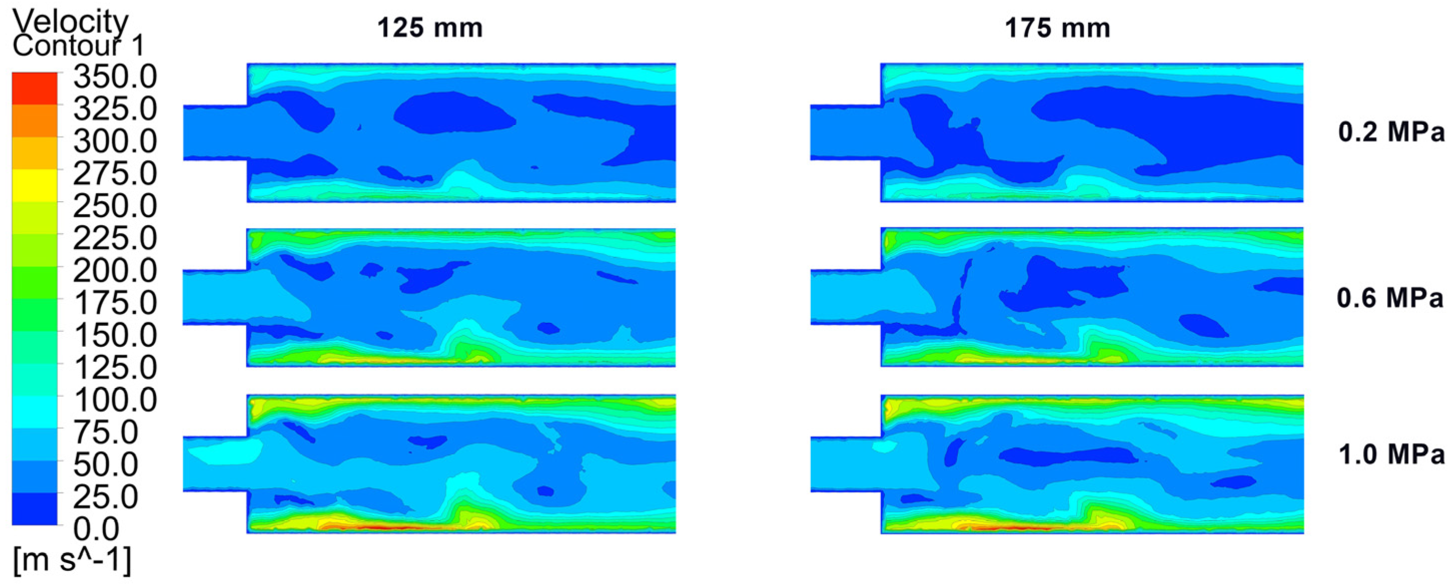
3.4. Contour Graphs of Axial and Radial Velocity Distribution

The compressed gas enters the vortex chamber tangentially from the swirl flow pipe inlet, the gas expansion performs work, and part of the pressure potential energy is converted into kinetic energy at the inlet. The kinetic energy forms a high-speed vortex flow in the pipe (Figure 10), increasing the temperature at the wall of the pipe, and produce a pressure gradient from the outer edge of the tube to the axial area. When the inlet pressure reaches 1 MPa, the inlet of the swirl flow pipe is depressurized, expanded, and accelerated to a critical state at the minimum cross-section. The depressurization continues to reach a supersonic state in the vortex chamber. From the numerical simulation results, it can be seen that the supersonic fluid will appear only when the pressure at the swirl flow pipe inlet is high enough. The pressure gradient between the hot-end valve and the vortex chamber is caused by the action of the hot-end valve, which in turn leads to backflow in the axial region. The high-speed airflow is in a cyclonic state while moving toward the hot-end valve, so the vortex phenomenon occurs in the swirl flow pipe (Figure 11). Figure 12 shows the distribution curve of the axial velocity of the swirl flow pipe. From Figure 12, it can be seen that the vortex velocity gradually decreases along with increased axial distance in the direction of the hot-end tube. The velocity variation in the axial region are low, and the energy separation is precisely due to the interaction between the positive and counter-rotating fluids. Figure 13 shows a three-dimensional streamline diagram of the swirl flow pipe, from which it can be seen that the axial velocity gradually decreases from the swirl flow pipe inlet to the direction of the hot-end valve and gradually increases as the inlet pressure increases. A long hot-end tube facilitates an increase in axial velocity.

Therefore, the axial velocity is a direct factor affecting the separation of hot and cold airflow in the swirl flow pipe. The interaction between the axially-oriented downstream and counter flows is a large contributor to the energy exchange in the swirl flow pipe, so it is vital to explore axial velocity. As the inlet pressure increases, the inlet velocity also increases, as shown in the blue part of Figure 11. As there is only one inlet nozzle for the swirl flow pipe, the sidewall of the vortex chamber near the inlet has the highest air velocity. To improve the durability of the swirl flow pipe, the vortex chamber can be designed with stronger materials, or the number of inlet nozzles can be increased to reduce erosion of the sidewall of the vortex chamber.

Figure 14 and Figure 15 show the axial circumferential velocity distribution of two different lengths of swirl flow pipes. The fluid entering the tube tangentially from the nozzle spontaneously generates free vortex flow along the outer edge of the swirl flow pipe (due to the restraining effect of the outer edge of the tube), while the counterflow fluid region away from the outer edge of the tube forms a forced vortex flow (due to the interaction between the inner and outer fluid).

3.5. Effect of Inlet Pressure on Radial Velocity

Figure 16 illustrates a three-dimensional model based on a physical drawing of the swirl flow pipe. The 3-dimensional model is defined by the Z-axis in the direction of the hot-end tube, the Y-axis in the direction of the swirl flow pipe inlet, and the X-axis perpendicular to the direction of the hot-end tube, with the origin coordinates placed in the middle of the swirl flow pipe.

The high-pressure flow passes through the inlet nozzle of the swirl flow pipe into the main tube. As the swirl flow pipe has no external source of work or heat, the pressure at the inlet is the only energy source available. The bulk of the pressure drop occurs in the nozzle, where the velocity increases dramatically, and a cyclonic flow is established. Figure 17 shows that as the swirl flow pipe inlet pressure continues to increase, the inlet radial cyclonic velocity rises, but the magnitude of the change decreases. The tangential velocity of the core flow is lower than that of the peripheral flow. It can be seen that the tangential velocity increases in the positive and negative Y-direction along the radius of the tube. The maximum velocity in the negative direction of the X-axis is greater than the maximum velocity in the positive direction, mainly because the former velocity is the velocity at the inlet of the swirl flow pipe into the vortex chamber, as shown in Figure 10. The pressure potential energy of the gas at the inlet is converted into kinetic energy, and the velocity rises sharply; this is the maximum velocity inside the swirl flow pipe. Figure 17 shows a gradual increase in tangential velocity from the center of the shaft to the outer edge of the swirl flow pipe, the low-velocity region at the center of the shaft gradually increases in the direction of the hot-end tube, indicating a gradual decrease in pressure along the hot-end tube.

Figure 17 also shows that the tangential velocity increases from the center of the axis to the outer edge of the swirl flow pipe in the same axial section; the tangential velocity also rises gradually with increasing pressure, but the increment decreases. There are significant differences in the tangential velocity in different axial sections. Along the hot-end tube, the tangential velocity becomes progressively weaker due to the fluid pressure difference and kinetic energy loss. As the fluid enters the vortex chamber tangentially, the fluid flows tangentially along the outer edge, so the pressure at the outer edge is higher than the pressure in the axial region. At different axial cross-sections, the exchange of work, kinetic energy, and heat (during the flow process) result in a reduction in pressure and, therefore, a reduction in tangential velocity. Figure 18 indicates that the effect of swirl flow pipe length on radial velocity is smaller for the same inlet pressure, as seen in the three plots, where the velocity of the swirl flow pipe with a tube length of 175 mm is slightly higher than that of the swirl flow pipe with a tube length of 125 mm. This leads to the conclusion that it is the number of swirl flow pipe inlets and the vortex chamber diameter, rather than the length of the swirl flow pipe hot end, that affects the radial velocity of the vortex chamber.

4. Conclusions

In the present study, numerical simulations were carried out on the designed swirl flow pipes of 125 and 175 mm length, and the process of energy separation was discussed. By varying the inlet pressure and comparing the maximum and minimum temperatures of two swirl flow pipes of different lengths, it can be concluded that the low-temperature effect of the swirl flow pipe first increases, then decreases, with increasing inlet pressure. Furthermore, pressure has a greater influence (on temperature) than pipe length. At an inlet pressure of 0.8 MPa, the lowest axial temperature of the 125 mm swirl flow pipe was 252.4 K, and the lowest axial temperature of the 175 mm pipe was 246.0 K. In summary, increasing the pressure increases the energy separation effect of the swirl flow pipe, all other things being equal. Moreover, as the pressure increases, the heating effect of the swirl flow pipe is greater than the cooling effect. The tube length also has little effect on the radial velocity of the swirl flow pipe but increases the maximum temperature. The numerical simulation found that as the pressure increases, the single-nozzle swirl flow pipe becomes more heavily burdened, and the vortex chamber wears out. A solution can be found by studying the effect of the number of swirl flow pipe inlets. When the swirl flow pipe is used as refrigeration equipment, the inlet pressure of the swirl flow pipe can be increased appropriately to obtain a lower thermodynamic temperature. When the swirl flow pipe is used as heat-producing equipment, the maximum heat-producing temperature can be increased by appropriately increasing the tube length of the swirl flow pipe.

References

1. Guo, X.; Zhang, B.; Liu, B.; Xu, X. A critical review on the flow structure studies of Ranque–Hilsch vortex tubes. Int. J. Refrig. 2019, 104, 51–64. [Google Scholar] [CrossRef]
2. Sarkar, J. Cycle parameter optimization of vortex tube expansion transcritical CO2 system. Int. J. Therm. Sci. 2009, 48, 1823–1828. [Google Scholar] [CrossRef]
3. Bazgir, A.; Nabhani, N.; Bazooyar, B.; Heydari, A. Computational Fluid Dynamic Prediction and Physical Mechanisms Consideration of Thermal Separation and Heat Transfer Processes Inside Divergent, Straight, and Convergent Ranque–Hilsch Vortex Tubes. J. Heat Transfer. 2019, 141. [Google Scholar] [CrossRef]
4. Wu, Y.T.; Ding, Y.; Ji, Y.B.; Ma, C.F.; Ge, M.C. Modification and experimental research on vortex tube. Int. J. Refrig. 2007, 30, 1042–1049. [Google Scholar] [CrossRef]
5. Kobiela, B.; Younis, B.A.; Weigand, B.; Neumann, O. A computational and experimental study of thermal energy separation by swirl. Int. J. Heat Mass Transfer. 2018, 124, 11–19. [Google Scholar] [CrossRef] [Green Version]
6. Behera, U.; Paul, P.J.; Kasthurirengan, S.; Karunanithi, R.; Ram, S.N.; Dinesh, K.; Jacob, S. CFD analysis and experimental investigations towards optimizing the parameters of Ranque–Hilsch vortex tube. Int. J. Heat Mass Transfer. 2005, 48, 1961–1973. [Google Scholar] [CrossRef] [Green Version]
7. Godbole, R.; Ramakrishna, P.A. Design guidelines for the vortex tube. Exp. Therm. Fluid Sci. 2020, 118. [Google Scholar] [CrossRef]
8. Hu, Z.; Li, R.; Yang, X.; Yang, M.; Day, R.; Wu, H. Energy separation for Ranque-Hilsch vortex tube: A short review. Therm. Sci. Eng. Prog. 2020, 19. [Google Scholar] [CrossRef]
9. Polat, K.; Kırmacı, V. Application of the output dependent feature scaling in modeling and prediction of performance of counter flow vortex tube having various nozzles numbers at different inlet pressures of air, oxygen, nitrogen and argon. Int. J. Refrig. 2011, 34, 1387–1397. [Google Scholar] [CrossRef]
10. Kırmacı, V. Exergy analysis and performance of a counter flow Ranque–Hilsch vortex tube having various nozzle numbers at different inlet pressures of oxygen and air. Int. J. Refrig. 2009, 32, 1626–1633. [Google Scholar] [CrossRef]
11. Polat, K.; Kırmacı, V. Determining of gas type in counter flow vortex tube using pairwise fisher score attribute reduction method. Int. J. Refrig. 2011, 34, 1372–1386. [Google Scholar] [CrossRef]
12. Kaya, H.; Günver, F.; Kirmaci, V. Experimental investigation of thermal performance of parallel connected vortex tubes with various nozzle materials. Appl. Therm. Eng. 2018, 136, 287–292. [Google Scholar] [CrossRef]
13. Gökçe, H. Optimization of Ranque–Hilsch vortex tube performances via Taguchi method. J. Braz. Soc. Mech. Sci. Eng. 2020, 42. [Google Scholar] [CrossRef]
14. Agrawal, N.; Naik, S.S.; Gawale, Y.P. Experimental investigation of vortex tube using natural substances. Int. Commun. Heat Mass Transfer. 2014, 52, 51–55. [Google Scholar] [CrossRef]
15. Aghagoli, A.; Sorin, M. Thermodynamic performance of a CO2 vortex tube based on 3D CFD flow analysis. Int. J. Refrig. 2019, 108, 124–137. [Google Scholar] [CrossRef]
16. Han, X.; Li, N.; Wu, K.; Wang, Z.; Tang, L.; Chen, G.; Xu, X. The influence of working gas characteristics on energy separation of vortex tube. Appl. Therm. Eng. 2013, 61, 171–177. [Google Scholar] [CrossRef]
17. Dincer, K.; Yilmaz, Y.; Berber, A.; Baskaya, S. Experimental investigation of performance of hot cascade type Ranque–Hilsch vortex tube and exergy analysis. Int. J. Refrig. 2011, 34, 1117–1124. [Google Scholar] [CrossRef]
18. Pourmahmoud, N.; Feyzi, A.; Orang, A.A.; Paykani, A. A parametric study on the performance of a Ranque-Hilsch vortex tube using a CFD-based approach. Mech. Ind. 2015, 16. [Google Scholar] [CrossRef]
19. Bramo, A.R.; Pourmahmoud, N. CFD simulation of length to diameter ratio effects on the energy separation in a vortex tube. Therm. Sci. 2011, 15, 833–848. [Google Scholar] [CrossRef]
20. Rafiee, S.E.; Sadeghiazad, M.M. Experimental and 3D CFD analysis on optimization of geometrical parameters of parallel vortex tube cyclone separator. Aerosp. Sci. Technol. 2017, 63, 110–122. [Google Scholar] [CrossRef]
21. Valipour, M.S.; Niazi, N. Experimental modeling of a curved Ranque–Hilsch vortex tube refrigerator. Int. J. Refrig. 2011, 34, 1109–1116. [Google Scholar] [CrossRef]
Figure 1. Physical model dimensions of the swirl flow pipe. All dimensions are in mm.
Applsci 11 09386 g001
Figure 2. Simplified 3D model of swirl flow pipe. Dimensions are the same as those shown in Figure 1.
Applsci 11 09386 g002
Figure 3. Meshing of the swirl flow pipe.
Applsci 11 09386 g003
Figure 4. Comparison of experimental data and CFD simulation results for swirl flow pipes of length 125 mm.
Applsci 11 09386 g004
Figure 5. Comparison of experimental data and CFD simulation results for swirl flow pipes of length 175 mm.
Applsci 11 09386 g005
Figure 6. Effect of inlet pressure and length of swirl flow pipe hot-end tube on cold outlet temperature.
Applsci 11 09386 g006
Figure 7. Effect of inlet pressure and length of swirl flow pipe hot-end tube on hot end temperature.
Applsci 11 09386 g007
Figure 8. Effect of inlet pressure and hot-end tube length ((a), 125 mm swirl flow pipe. (b), 175 mm swirl flow pipe) on axial outlet temperature.
Applsci 11 09386 g008
Figure 9. Effect of inlet pressure and hot-end tube length on radial temperature distribution.
Applsci 11 09386 g009
Figure 10. Radial velocity distribution of swirl flow pipes at different pressures.
Applsci 11 09386 g010
Figure 11. Axial velocity distribution of the swirl flow pipes at different inlet pressures.
Applsci 11 09386 g011
Figure 12. Axial velocity distribution curve of swirl flow pipes under different inlet pressures.
Applsci 11 09386 g012
Figure 13. Schematic diagram of the three-dimensional streamline diagram of a swirl flow pipe.
Applsci 11 09386 g013
Figure 14. Circumferential velocity distribution of 125 mm swirl flow pipe.
Applsci 11 09386 g014
Figure 15. Circumferential velocity distribution of 175 mm swirl flow pipe.
Applsci 11 09386 g015
Figure 16. Schematic diagram of 3-dimensional coordinates of the swirl flow pipe.
Applsci 11 09386 g016
Figure 17. Radial velocity distribution along the X-position at different inlet pressures.
Applsci 11 09386 g017
Figure 18. Radial velocity distribution for two lengths of swirl flow pipe at the same pressure.
Applsci 11 09386 g018