
A Combined Forecasting System Based on Modified Multi-Objective Optimization for Short-Term Wind Speed and Wind Power Forecasting

Abstract
:1. Introduction
- (1)
- For physical methods, to attain effective forecasting results, information on a range of physical factors is needed, rather than information on just a single factor such as the wind speed time series; thus, these meteorological models cannot generate forecasts simply [15]. In addition, physical models are not proficient in dealing with short-term series and involve a complex calculation process and high expansion costs, which all contribute to significant forecasting errors [16]. Physical models necessitate the gathering of numerical physical variables, such as the horizontal pressure gradient, geostrophic force, and fractionate to undergo wind speed forecasting [17]. However, the complex calculation and polytrophic processes involved are not only time consuming but create the risk of forecasting error [18].
- (2)
- With sufficient accessible spatial and temporal information from multiple wind farms, a few spatio-temporal prediction methodologies have been able to be investigated in recent studies. The spatio-temporal characteristics of wind speed are extracted by an undirected graph of wind farms [19]. A hybrid support vector machine forecasting model is proposed, which is based on the spatio-temporal and grey wolf optimization, to forecast wind power for multiple wind farms [20]. Ref. [21] uses copula theory and Bayesian theory to simulate spatio-temporal correlations between wind farms and deduce a conditional distribution of aggregated wind power. A probabilistic wind speed prediction approach was presented in Ref. [22] based on a spatio-temporal neural network (STNN) and variational Bayesian inference. With feeding of both the spatial and temporal information into the forecasting model, these methods have achieved a better forecasting performance. Nevertheless, most of these forecasting models often collected the wind speed information from different wind farms indiscriminately, and to some extent, the implicit spatial correlations cannot be fully exploited in the original wind speed data. Also, the thorny multi-dimensional computing problem caused by the large amount of wind speed data from multiple wind farms needs to be solved in an effective way.
- (3)
- Typical statistical methods can yield excellent forecasting results under the assumption that the input series was recorded under normal conditions [23]; however, nonlinearity, noise, instability, fluctuations, and other features within the raw time series are always difficult to control, resulting in a lack of modeling information. Therefore, such methods often result in bad short-term wind speed forecasting performance, especially in multistep-ahead forecasting [24]. In addition, historical data are utilized for statistical modeling methods, and only potential linear correlations between the variables and future forecasts are revealed; such models are unable to obtain a good forecasting performance within the required limits [25]. Statistical models, including typical autoregressive moving average family models (e.g., AR [26], MA, ARMA [27], autoregressive integrated moving average models (ARIMA) [28], SARIMA, etc.), exponential smoothing [29], Kalman filtering [30], vector autoregression structures for very short-term wind power forecasting [31], and autoregressive conditional heteroskedastic family models (e.g., ARCH, GARCH, and EARCH) [32] utilize significant amounts of historical data for wind speed forecasting with no consideration of other potential influencing factors to support the stochastic process. Meanwhile, a spatial-temporal forecasting method based on the vector autoregression framework has been proposed for renewable forecasting [33]. Generally, statistical methods work well for approaching linear features; however, they tend to fail when it comes to nonlinear problems due to the linear assumptions of the models [34].
- (4)
- Fortunately, the timely emergence of artificial intelligence (AI) arithmetic, subsuming artificial neural networks (ANNs) [35], support vector machines (SVMs) [36], deep neural networks [37], and fuzzy logical methods (FLMs) [38] have efficiently remedied the flaws in the wind speed forecasting territory in recent years [39]. However, because of the inherent disadvantages of each model and the boom in the integration of wind power into the grid system, a variety of hybrid and combined models with promising forecasting potentials have been created [40]. Generally, artificial intelligence methods can achieve greater forecasting accuracy than physical or statistical models [41]; however, they also possess insurmountable drawbacks. ANNs have been extensively studied and applied to explore the complexity of wind speed forecasting; however, their performance mostly relies on training sets, which can result in a focus on local optima, over-fitting, and a reduction in the convergence rate [42].
- (5)
- Differently to conventional or single models, hybrid models can reduce the current shortcomings associated with the forecasting of irregular, fluctuant, and nonstationary time series with noise or unpredictable components. In this regard, significant hybrid models have recently been launched [43]. Hybrid methods integrate different single algorithms to achieve a superior forecasting performance, and can overcome defects in AI models (e.g., falling into local minima, over-fitting, etc.)—greatly improving the accuracy of continuous fluctuant wind speed forecasting and providing better validity and stability than a single model [44]. Recently, the use of hybrid methods in the wind speed forecasting field has been widespread. Jiang et al. [45] proposed a hybrid model consisting of a grey correlation analysis, cuckoo search algorithm, and v-SVM (v-support vector machine). Dong et al. [46] proposed a hybrid preprocessing strategy coupled with an optimized local linear fuzzy neural network for wind power forecasting. It has been proven that this is a effective approach for predicting wind power. In 2017, Hu et al. [47] proposed a novel approach based on the Gaussian process with a t-observation model for short-term wind speed forecasting. Based on a spatio-temporal method, in [48], the performance of predictive clustering trees with a new feature space for wind power forecasting was investigated. The results showed that the proposed model achieved a satisfactory level of point forecasting accuracy and interval forecasting performance. A forecasting framework has been proposed in 2021 [49], that is multi-layer stacked bidirectional long/short-term memory (LSTM)-based for short-term time series forecasting. After being studied extensively, it is clear that no arithmetic method is omnipotent across all data cases. In future research, individual statistical models and artificial intelligence algorithms will be integrated to improve the precision of wind speed forecasting—these are referred to as hybrid models [50].
- (1)
- To achieve accurate and stable forecasting of short-term wind speed and wind power, a robust, novel, combined system based on three modules was developed in this study. This novel hybrid system for forecasting short-term wind speed and wind power includes a data preprocessing module, a forecast optimization module, and an evaluation module. The excellent performances of these algorithms are combined to provide accurate and stable results for multi-step wind speed forecasting.
- (2)
- To effectively eliminate fluctuations in the original time series and avoid the limitations of a single algorithm, a new data preprocessing step was proposed. This was shown to decrease uncertainty and irregularity in the wind speed times series. SSA-EEMD, a powerful secondary denoising algorithm, was used to decompose and further denoise the actual wind speed time series. These steps were found to successfully overcome the limitations of single SSA algorithms.
- (3)
- To overcome the disadvantages of individual models, multi models were used to forecast the wind speed and wind power. To consider the nonlinear characteristics of wind speed and wind power time series, seven artificial neural networks (ANNs) were employed to forecast two types of time series, and five optimal hybrid models were selected based on the accuracy of data testing by hybrid models to form a combined model and act as sub-models.
- (4)
- To further improve forecasting accuracy and stability, the multi-objective dragonfly algorithm was used to determine the optimal weight of the combined model. In the optimization process, the optimized parameters were found to not only have good accuracy, but they also ensured that the output results had a high level of stability. Therefore, this paper used the multi-objective optimization algorithm to optimize the weight of the combined model.
- (5)
- A more scientific and comprehensive forecasting evaluation method was conducted to estimate the forecasting performance of the developed forecasting system in the model evolution module. Interval forecasting was used to assess the uncertainty of the combined model, and this indicated that the forecasting results of the proposed combined model were accurate and stabilized in an all-around manner. Additionally, the Diebold–Mariano test and Wilcoxon rank-sum test were implemented to further analyze the forecasting accuracy of each model.
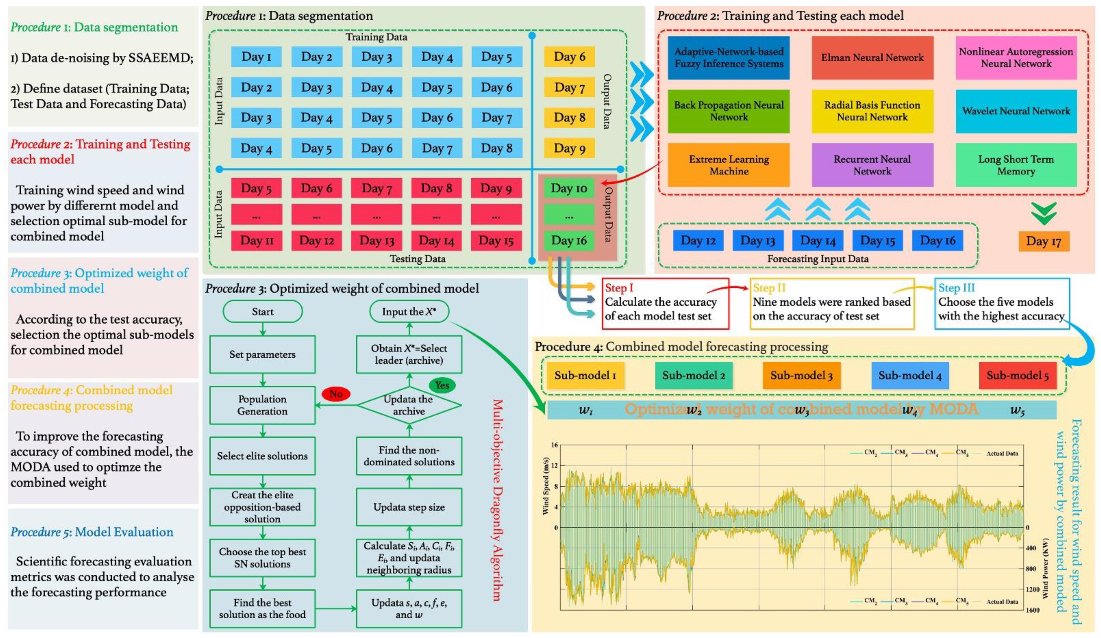
2. Flow of the Proposed Combined Model
- Procedure 1: Data Pretreatment
- Procedure 2: Prediction of Hybrid Models
- Procedure 3: Establishment of the Proposed Combined System
- Procedure 4: Wind Speed and Wind Power Forecasting
- Procedure 5: Model Evaluation
3. Experiment and Results
3.1. Data Acquisition
3.2. Experimental Setup
3.3. Performance Metrics and Benchmark Model
3.4. Parameter Setting
3.5. Experimental Results and Analysis
3.5.1. Experiment I: The Forecasting Performance of the Combined Models Optimized by Different Optimization Algorithms
3.5.2. Experiment II: The Forecasting Performance of Combined Models Optimized by Different Optimization Algorithms
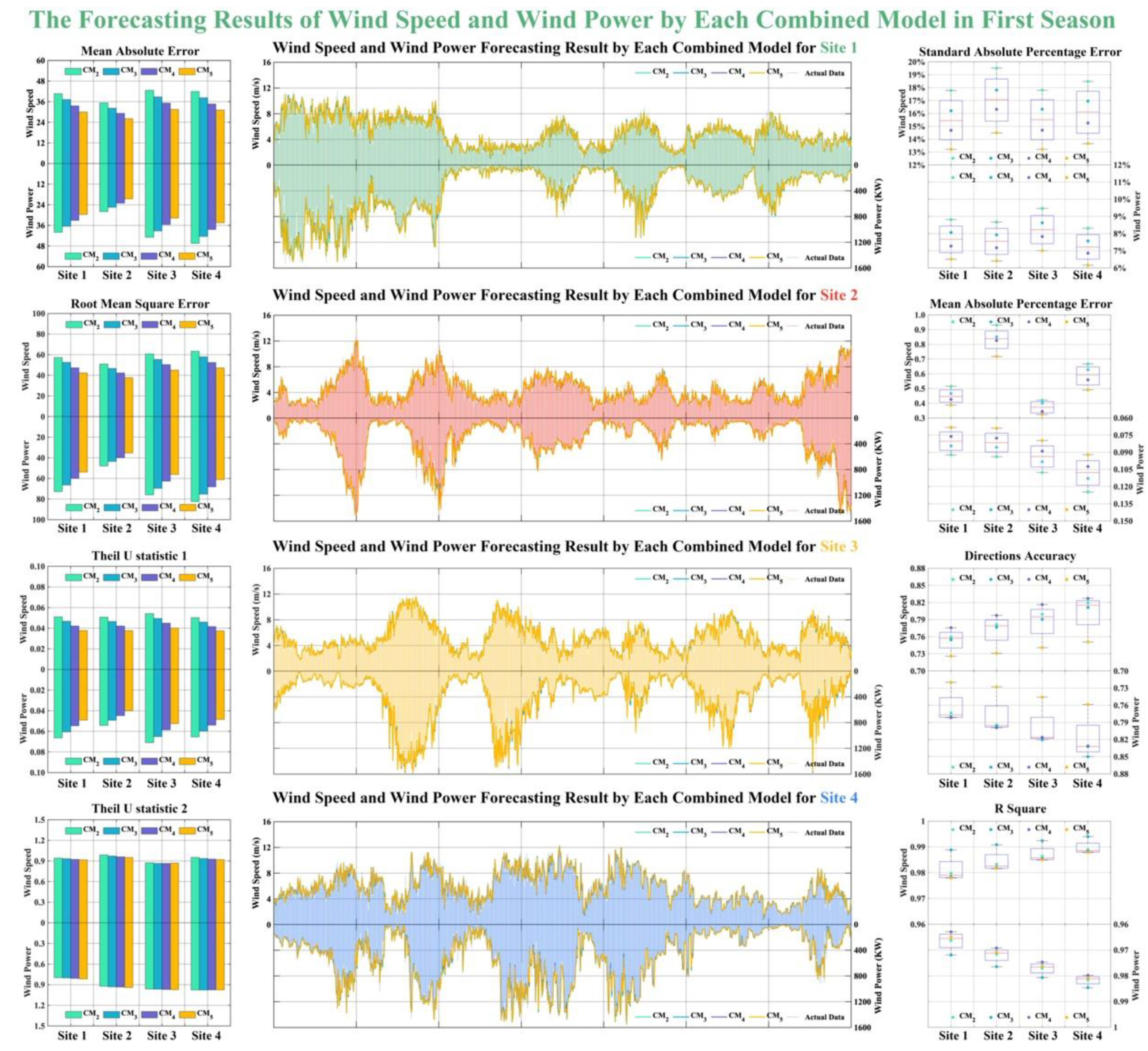
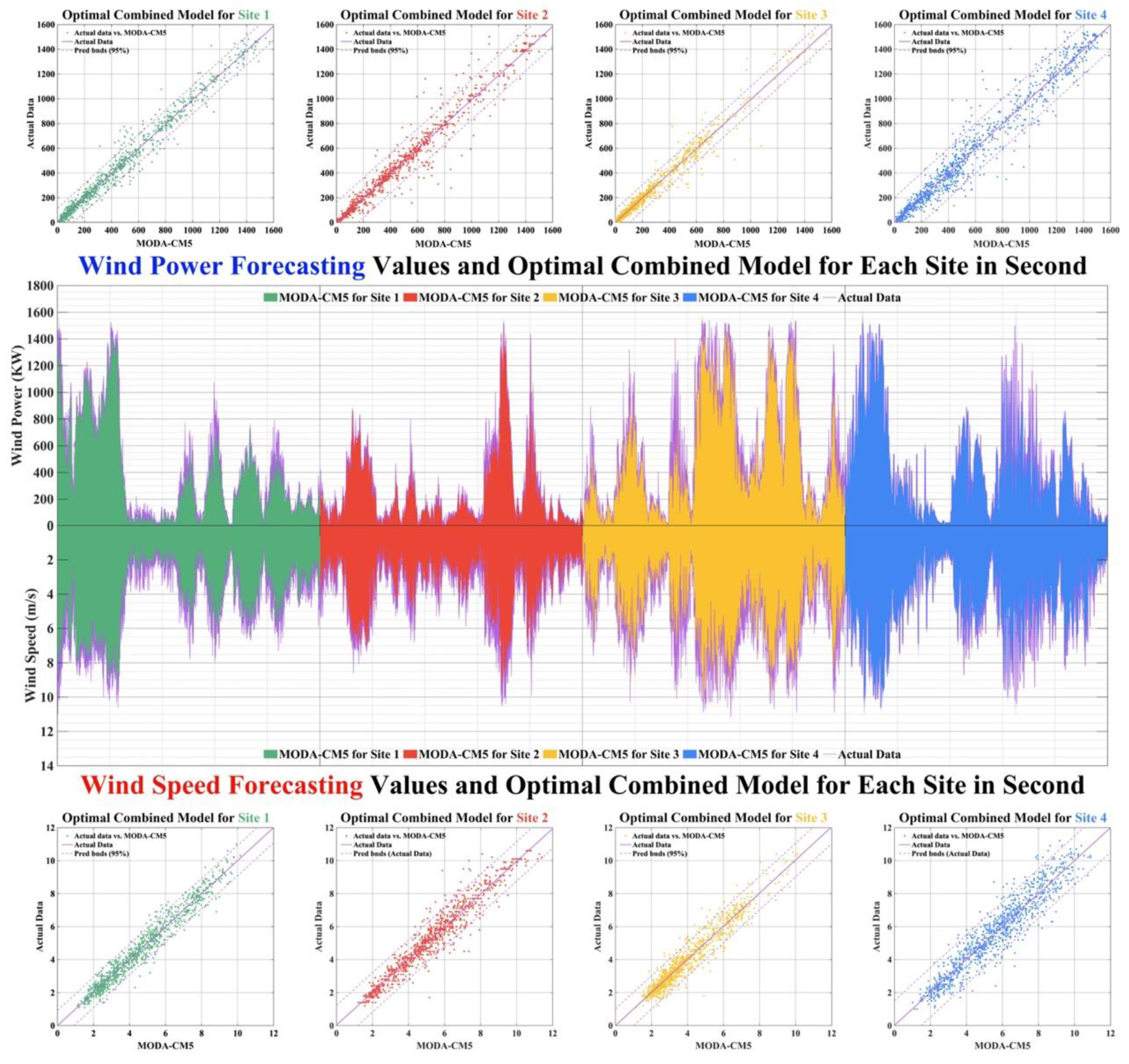
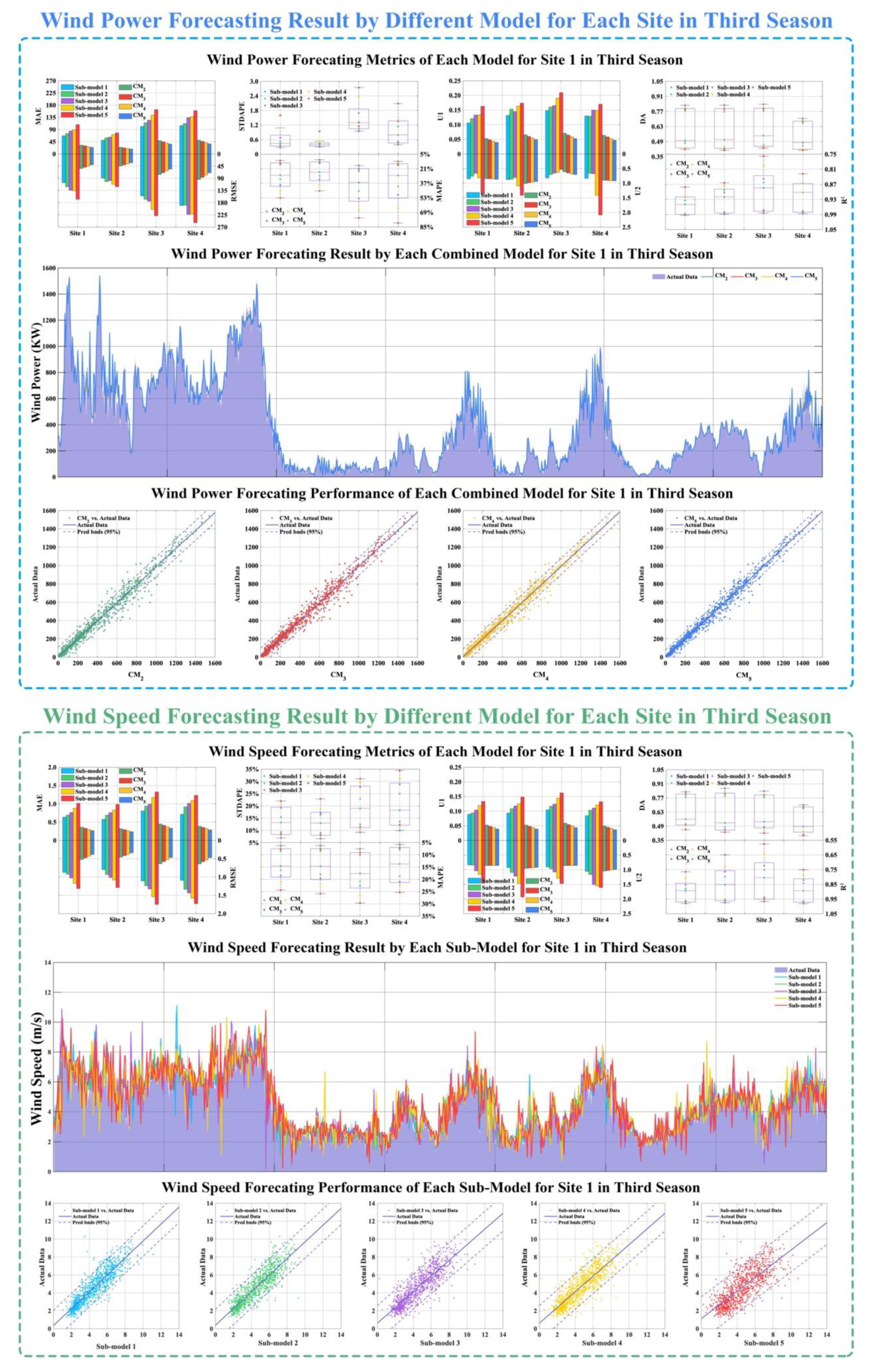
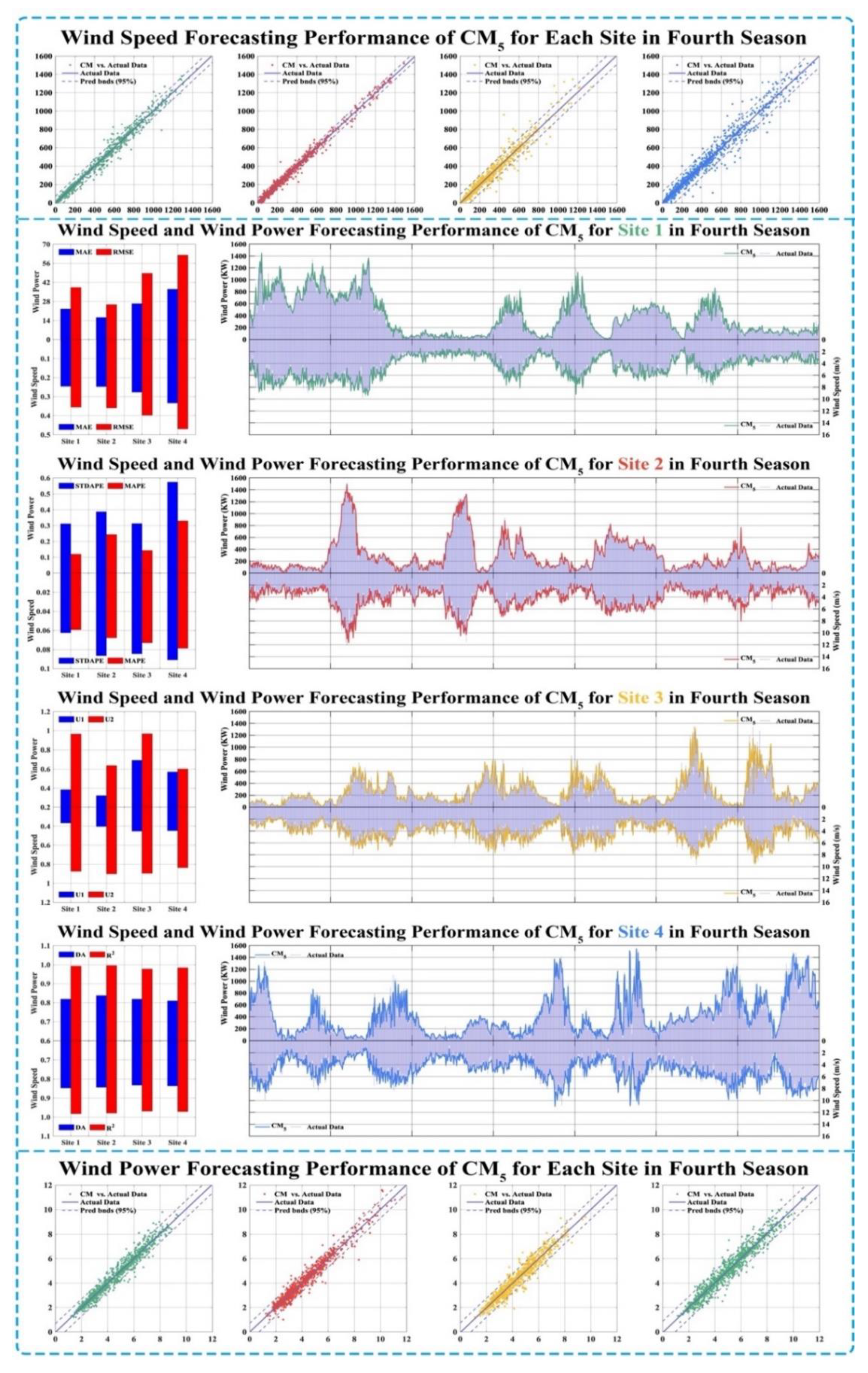
3.5.3. Experiment III: Verification of the Performance of the Combined Model Based on Five Sub-Models and Optimized by MODA
4. Discussion
4.1. Significance Test between Forecasting Values and Actual Data
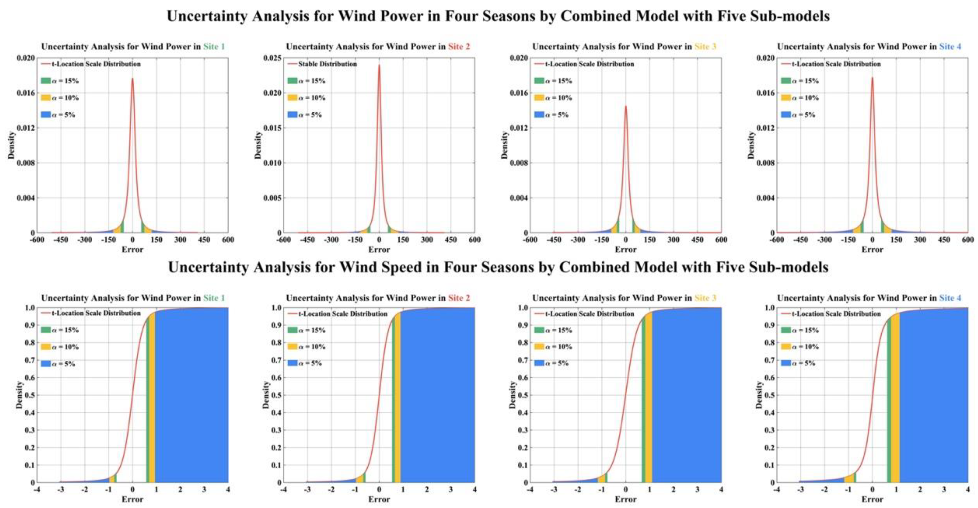
4.2. Uncertainty Analysis
5. Conclusions
Author Contributions
Funding
Conflicts of Interest
Appendix A
Modified Multi-Objective Dragonfly Algorithm
- (1)
- Elite Opposition Learning Strategy
- (2)
- Steps-based Strategy based on an Exponential Function

| Site | Metric | Wind Speed Forecasting Results | Wind Power Forecasting Results | ||||||||
| LSTM | WNN | ANFIS | RNN | ELM | LSTM | Elman | BPNN | RBFNN | SVM | ||
| Site 1 | MAE | 0.7128 | 0.8047 | 0.9306 | 0.9952 | 1.1224 | 72.7578 | 84.7192 | 94.2429 | 100.1841 | 123.008 |
| RMSE | 0.9969 | 1.0498 | 1.213 | 1.316 | 1.4909 | 123.6352 | 138.1371 | 150.2004 | 159.6466 | 191.7045 | |
| STDAPE | 14.22% | 15.16% | 17.65% | 18.85% | 20.90% | 80.87% | 136.27% | 153.49% | 172.28% | 260.26% | |
| DA | 53.23% | 47.27% | 44.39% | 47.47% | 44.59% | 50.05% | 44.49% | 45.08% | 43.40% | 40.81% | |
| U1 | 0.0902 | 0.0951 | 0.1093 | 0.1182 | 0.1329 | 0.1144 | 0.1281 | 0.1389 | 0.1467 | 0.1749 | |
| U2 | 0.8881 | 0.871 | 1.0413 | 1.085 | 1.4672 | 0.4916 | 0.5218 | 0.5837 | 0.6357 | 1.7005 | |
| MAPE | 14.91% | 17.05% | 20.06% | 21.49% | 24.03% | 28.53% | 35.87% | 37.62% | 43.22% | 55.27% | |
| R2 | 0.896 | 0.8831 | 0.8451 | 0.8182 | 0.7771 | 0.9411 | 0.9257 | 0.9121 | 0.9022 | 0.8603 | |
| Site | Metric | LSTM | WNN | ELM | RNN | ANFIS | LSTM | Elman | BPNN | SVM | RBFNN |
| Site 2 | MAE | 0.6592 | 0.7582 | 0.8299 | 0.9609 | 1.113 | 55.2501 | 64.6423 | 68.5449 | 81.2518 | 92.9089 |
| RMSE | 0.9157 | 1.0199 | 1.1101 | 1.2878 | 1.4649 | 94.3334 | 101.4713 | 107.9959 | 129.0841 | 146.0998 | |
| STDAPE | 15.65% | 18.03% | 18.53% | 20.95% | 26.19% | 105.16% | 234.08% | 255.50% | 348.94% | 427.78% | |
| DA | 52.33% | 46.57% | 47.57% | 43.00% | 42.60% | 50.35% | 42.30% | 44.69% | 41.31% | 39.82% | |
| U1 | 0.0926 | 0.1028 | 0.1118 | 0.1291 | 0.1459 | 0.1092 | 0.1169 | 0.1233 | 0.1476 | 0.1652 | |
| U2 | 1.0602 | 1.1315 | 1.2836 | 1.5189 | 1.8958 | 0.827 | 0.7993 | 0.7507 | 0.7423 | 0.6758 | |
| MAPE | 15.81% | 18.63% | 20.35% | 23.44% | 27.72% | 31.61% | 45.31% | 52.43% | 62.54% | 75.86% | |
| R2 | 0.9078 | 0.8857 | 0.8658 | 0.8221 | 0.7738 | 0.9575 | 0.9499 | 0.9432 | 0.918 | 0.8969 | |
| Site | Metric | LSTM | RNN | ELM | WNN | ANFIS | Elman | LSTM | BPNN | RBFNN | ANFIS |
| Site 3 | MAE | 0.7401 | 0.8572 | 0.9891 | 1.1429 | 1.2817 | 86.0772 | 102.83 | 110.7717 | 124.926 | 141.6915 |
| RMSE | 1.0265 | 1.1234 | 1.2926 | 1.4726 | 1.6495 | 143.5346 | 167.6258 | 174.9203 | 191.9277 | 213.2843 | |
| STDAPE | 16.57% | 17.86% | 22.35% | 23.63% | 27.92% | 184.14% | 241.75% | 270.58% | 331.04% | 381.07% | |
| DA | 52.04% | 46.38% | 43.50% | 40.32% | 42.01% | 52.14% | 44.89% | 44.79% | 45.38% | 41.81% | |
| U1 | 0.0921 | 0.1009 | 0.1155 | 0.1309 | 0.1453 | 0.1367 | 0.1592 | 0.165 | 0.1777 | 0.1965 | |
| U2 | 0.9028 | 1.0113 | 1.1226 | 1.2138 | 1.43 | 0.7837 | 0.8137 | 0.7846 | 0.7471 | 0.7233 | |
| MAPE | 16.43% | 18.98% | 22.27% | 25.56% | 29.17% | 38.51% | 48.10% | 55.41% | 64.25% | 75.54% | |
| R2 | 0.8932 | 0.872 | 0.8308 | 0.7842 | 0.745 | 0.9216 | 0.893 | 0.8834 | 0.8661 | 0.8373 | |
| Site | Metric | ANFIS | WNN | ELM | RNN | NARNN | ANFIS | BPNN | RBFNN | Elman | GRNN |
| Site 4 | MAE | 0.783 | 0.8931 | 1.0345 | 1.18 | 1.3166 | 90.0454 | 107.0139 | 117.4349 | 132.8439 | 154.0333 |
| RMSE | 1.1462 | 1.2293 | 1.4323 | 1.6254 | 1.803 | 152.6258 | 173.0959 | 180.8868 | 213.9421 | 228.7902 | |
| STDAPE | 18.73% | 21.71% | 25.73% | 27.44% | 28.79% | 64.24% | 79.57% | 123.60% | 153.34% | 149.54% | |
| DA | 51.14% | 48.36% | 43.89% | 42.40% | 39.52% | 48.56% | 44.19% | 46.08% | 43.59% | 41.51% | |
| U1 | 0.0914 | 0.098 | 0.1136 | 0.1286 | 0.1422 | 0.1235 | 0.14 | 0.1451 | 0.1679 | 0.1794 | |
| U2 | 1.1756 | 1.0218 | 1.2242 | 1.4279 | 1.5687 | 0.9525 | 0.9708 | 0.998 | 0.6264 | 0.7754 | |
| MAPE | 15.00% | 17.86% | 20.74% | 23.37% | 25.91% | 29.34% | 36.77% | 45.06% | 53.03% | 61.99% | |
| R2 | 0.8821 | 0.8631 | 0.8156 | 0.7734 | 0.7272 | 0.9227 | 0.8995 | 0.8909 | 0.8598 | 0.8351 | |
| Site | Metric | Wind Speed Forecasting Results | Wind Power Forecasting Results | ||||||||
| LSTM | WNN | RNN | ANFIS | ELM | LSTM | Elman | BPNN | RBFNN | SVM | ||
| Site 1 | MAE | 0.7128 | 0.8047 | 0.9306 | 0.9952 | 1.1224 | 72.7578 | 84.7192 | 94.2429 | 100.1841 | 123.008 |
| RMSE | 0.9969 | 1.0498 | 1.213 | 1.316 | 1.4909 | 123.6352 | 138.1371 | 150.2004 | 159.6466 | 191.7045 | |
| STDAPE | 14.22% | 15.16% | 17.65% | 18.85% | 20.90% | 80.87% | 136.27% | 153.49% | 172.28% | 260.26% | |
| DA | 53.23% | 47.27% | 44.39% | 47.47% | 44.59% | 50.05% | 44.49% | 45.08% | 43.40% | 40.81% | |
| U1 | 0.0902 | 0.0951 | 0.1093 | 0.1182 | 0.1329 | 0.1144 | 0.1281 | 0.1389 | 0.1467 | 0.1749 | |
| U2 | 0.8881 | 0.871 | 1.0413 | 1.085 | 1.4672 | 0.4916 | 0.5218 | 0.5837 | 0.6357 | 1.7005 | |
| MAPE | 14.91% | 17.05% | 20.06% | 21.49% | 24.03% | 28.53% | 35.87% | 37.62% | 43.22% | 55.27% | |
| R2 | 0.896 | 0.8831 | 0.8451 | 0.8182 | 0.7771 | 0.9411 | 0.9257 | 0.9121 | 0.9022 | 0.8603 | |
| Site | Metric | LSTM | ELM | RNN | WNN | ANFIS | LSTM | Elman | BPNN | SVM | RBFNN |
| Site 2 | MAE | 0.6592 | 0.7582 | 0.8299 | 0.9609 | 1.113 | 55.2501 | 64.6423 | 68.5449 | 81.2518 | 92.9089 |
| RMSE | 0.9157 | 1.0199 | 1.1101 | 1.2878 | 1.4649 | 94.3334 | 101.4713 | 107.9959 | 129.0841 | 146.0998 | |
| STDAPE | 15.65% | 18.03% | 18.53% | 20.95% | 26.19% | 105.16% | 234.08% | 255.50% | 348.94% | 427.78% | |
| DA | 52.33% | 46.57% | 47.57% | 43.00% | 42.60% | 50.35% | 42.30% | 44.69% | 41.31% | 39.82% | |
| U1 | 0.0926 | 0.1028 | 0.1118 | 0.1291 | 0.1459 | 0.1092 | 0.1169 | 0.1233 | 0.1476 | 0.1652 | |
| U2 | 1.0602 | 1.1315 | 1.2836 | 1.5189 | 1.8958 | 0.827 | 0.7993 | 0.7507 | 0.7423 | 0.6758 | |
| MAPE | 15.81% | 18.63% | 20.35% | 23.44% | 27.72% | 31.61% | 45.31% | 52.43% | 62.54% | 75.86% | |
| R2 | 0.9078 | 0.8857 | 0.8658 | 0.8221 | 0.7738 | 0.9575 | 0.9499 | 0.9432 | 0.918 | 0.8969 | |
| Site | Metric | LSTM | WNN | ELM | RNN | ANFIS | LSTM | Elman | BPNN | ANFIS | SVM |
| Site 3 | MAE | 0.7401 | 0.8572 | 0.9891 | 1.1429 | 1.2817 | 86.0772 | 102.83 | 110.7717 | 124.926 | 141.6915 |
| RMSE | 1.0265 | 1.1234 | 1.2926 | 1.4726 | 1.6495 | 143.5346 | 167.6258 | 174.9203 | 191.9277 | 213.2843 | |
| STDAPE | 16.57% | 17.86% | 22.35% | 23.63% | 27.92% | 184.14% | 241.75% | 270.58% | 331.04% | 381.07% | |
| DA | 52.04% | 46.38% | 43.50% | 40.32% | 42.01% | 52.14% | 44.89% | 44.79% | 45.38% | 41.81% | |
| U1 | 0.0921 | 0.1009 | 0.1155 | 0.1309 | 0.1453 | 0.1367 | 0.1592 | 0.165 | 0.1777 | 0.1965 | |
| U2 | 0.9028 | 1.0113 | 1.1226 | 1.2138 | 1.43 | 0.7837 | 0.8137 | 0.7846 | 0.7471 | 0.7233 | |
| MAPE | 16.43% | 18.98% | 22.27% | 25.56% | 29.17% | 38.51% | 48.10% | 55.41% | 64.25% | 75.54% | |
| R2 | 0.8932 | 0.872 | 0.8308 | 0.7842 | 0.745 | 0.9216 | 0.893 | 0.8834 | 0.8661 | 0.8373 | |
| Site | Metric | ANFIS | WNN | ELM | RNN | NARNN | BPNN | Elman | LSTM | ANFIS | RBFNN |
| Site 4 | MAE | 0.783 | 0.8931 | 1.0345 | 1.18 | 1.3166 | 90.0454 | 107.0139 | 117.4349 | 132.8439 | 154.0333 |
| RMSE | 1.1462 | 1.2293 | 1.4323 | 1.6254 | 1.803 | 152.6258 | 173.0959 | 180.8868 | 213.9421 | 228.7902 | |
| STDAPE | 18.73% | 21.71% | 25.73% | 27.44% | 28.79% | 64.24% | 79.57% | 123.60% | 153.34% | 149.54% | |
| DA | 51.14% | 48.36% | 43.89% | 42.40% | 39.52% | 48.56% | 44.19% | 46.08% | 43.59% | 41.51% | |
| U1 | 0.0914 | 0.098 | 0.1136 | 0.1286 | 0.1422 | 0.1235 | 0.14 | 0.1451 | 0.1679 | 0.1794 | |
| U2 | 1.1756 | 1.0218 | 1.2242 | 1.4279 | 1.5687 | 0.9525 | 0.9708 | 0.998 | 0.6264 | 0.7754 | |
| MAPE | 15.00% | 17.86% | 20.74% | 23.37% | 25.91% | 29.34% | 36.77% | 45.06% | 53.03% | 61.99% | |
| R2 | 0.8821 | 0.8631 | 0.8156 | 0.7734 | 0.7272 | 0.9227 | 0.8995 | 0.8909 | 0.8598 | 0.8351 | |
| Site | Metric | Wind Speed Forecasting Results | Wind Power Forecasting Results | ||||||||
| LSTM | WNN | ANFIS | RNN | ELM | LSTM | Elman | BPNN | RBFNN | SVM | ||
| Site 1 | MAE | 0.7128 | 0.8047 | 0.9306 | 0.9952 | 1.1224 | 72.7578 | 84.7192 | 94.2429 | 100.1841 | 123.008 |
| RMSE | 0.9969 | 1.0498 | 1.213 | 1.316 | 1.4909 | 123.6352 | 138.1371 | 150.2004 | 159.6466 | 191.7045 | |
| STDAPE | 14.22% | 15.16% | 17.65% | 18.85% | 20.90% | 80.87% | 136.27% | 153.49% | 172.28% | 260.26% | |
| DA | 53.23% | 47.27% | 44.39% | 47.47% | 44.59% | 50.05% | 44.49% | 45.08% | 43.40% | 40.81% | |
| U1 | 0.0902 | 0.0951 | 0.1093 | 0.1182 | 0.1329 | 0.1144 | 0.1281 | 0.1389 | 0.1467 | 0.1749 | |
| U2 | 0.8881 | 0.871 | 1.0413 | 1.085 | 1.4672 | 0.4916 | 0.5218 | 0.5837 | 0.6357 | 1.7005 | |
| MAPE | 14.91% | 17.05% | 20.06% | 21.49% | 24.03% | 28.53% | 35.87% | 37.62% | 43.22% | 55.27% | |
| R2 | 0.896 | 0.8831 | 0.8451 | 0.8182 | 0.7771 | 0.9411 | 0.9257 | 0.9121 | 0.9022 | 0.8603 | |
| Site | Metric | LSTM | ELM | RNN | WNN | ANFIS | LSTM | Elman | BPNN | RBFNN | SVM |
| Site 2 | MAE | 0.6592 | 0.7582 | 0.8299 | 0.9609 | 1.113 | 55.2501 | 64.6423 | 68.5449 | 81.2518 | 92.9089 |
| RMSE | 0.9157 | 1.0199 | 1.1101 | 1.2878 | 1.4649 | 94.3334 | 101.4713 | 107.9959 | 129.0841 | 146.0998 | |
| STDAPE | 15.65% | 18.03% | 18.53% | 20.95% | 26.19% | 105.16% | 234.08% | 255.50% | 348.94% | 427.78% | |
| DA | 52.33% | 46.57% | 47.57% | 43.00% | 42.60% | 50.35% | 42.30% | 44.69% | 41.31% | 39.82% | |
| U1 | 0.0926 | 0.1028 | 0.1118 | 0.1291 | 0.1459 | 0.1092 | 0.1169 | 0.1233 | 0.1476 | 0.1652 | |
| U2 | 1.0602 | 1.1315 | 1.2836 | 1.5189 | 1.8958 | 0.827 | 0.7993 | 0.7507 | 0.7423 | 0.6758 | |
| MAPE | 15.81% | 18.63% | 20.35% | 23.44% | 27.72% | 31.61% | 45.31% | 52.43% | 62.54% | 75.86% | |
| R2 | 0.9078 | 0.8857 | 0.8658 | 0.8221 | 0.7738 | 0.9575 | 0.9499 | 0.9432 | 0.918 | 0.8969 | |
| Site | Metric | LSTM | RNN | WNN | ELM | ANFIS | LSTM | Elman | BPNN | RBFNN | SVM |
| Site 3 | MAE | 0.7401 | 0.8572 | 0.9891 | 1.1429 | 1.2817 | 86.0772 | 102.83 | 110.7717 | 124.926 | 141.6915 |
| RMSE | 1.0265 | 1.1234 | 1.2926 | 1.4726 | 1.6495 | 143.5346 | 167.6258 | 174.9203 | 191.9277 | 213.2843 | |
| STDAPE | 16.57% | 17.86% | 22.35% | 23.63% | 27.92% | 184.14% | 241.75% | 270.58% | 331.04% | 381.07% | |
| DA | 52.04% | 46.38% | 43.50% | 40.32% | 42.01% | 52.14% | 44.89% | 44.79% | 45.38% | 41.81% | |
| U1 | 0.0921 | 0.1009 | 0.1155 | 0.1309 | 0.1453 | 0.1367 | 0.1592 | 0.165 | 0.1777 | 0.1965 | |
| U2 | 0.9028 | 1.0113 | 1.1226 | 1.2138 | 1.43 | 0.7837 | 0.8137 | 0.7846 | 0.7471 | 0.7233 | |
| MAPE | 16.43% | 18.98% | 22.27% | 25.56% | 29.17% | 38.51% | 48.10% | 55.41% | 64.25% | 75.54% | |
| R2 | 0.8932 | 0.872 | 0.8308 | 0.7842 | 0.745 | 0.9216 | 0.893 | 0.8834 | 0.8661 | 0.8373 | |
| Site | Metric | ANFIS | RNN | WNN | ELM | NARNN | BPNN | ANFIS | Elman | RBFNN | GRNN |
| Site 4 | MAE | 0.783 | 0.8931 | 1.0345 | 1.18 | 1.3166 | 90.0454 | 107.0139 | 117.4349 | 132.8439 | 154.0333 |
| RMSE | 1.1462 | 1.2293 | 1.4323 | 1.6254 | 1.803 | 152.6258 | 173.0959 | 180.8868 | 213.9421 | 228.7902 | |
| STDAPE | 18.73% | 21.71% | 25.73% | 27.44% | 28.79% | 64.24% | 79.57% | 123.60% | 153.34% | 149.54% | |
| DA | 51.14% | 48.36% | 43.89% | 42.40% | 39.52% | 48.56% | 44.19% | 46.08% | 43.59% | 41.51% | |
| U1 | 0.0914 | 0.098 | 0.1136 | 0.1286 | 0.1422 | 0.1235 | 0.14 | 0.1451 | 0.1679 | 0.1794 | |
| U2 | 1.1756 | 1.0218 | 1.2242 | 1.4279 | 1.5687 | 0.9525 | 0.9708 | 0.998 | 0.6264 | 0.7754 | |
| MAPE | 15.00% | 17.86% | 20.74% | 23.37% | 25.91% | 29.34% | 36.77% | 45.06% | 53.03% | 61.99% | |
| R2 | 0.8821 | 0.8631 | 0.8156 | 0.7734 | 0.7272 | 0.9227 | 0.8995 | 0.8909 | 0.8598 | 0.8351 | |
| Site | Metric | Wind Speed Forecasting Results | Wind Power Forecasting Results | ||||||||
| LSTM | ANFIS | RNN | ELM | WNN | LSTM | Elman | BPNN | RBFNN | SVM | ||
| Site 1 | MAE | 0.7128 | 0.8047 | 0.9306 | 0.9952 | 1.1224 | 72.7578 | 84.7192 | 94.2429 | 100.1841 | 123.008 |
| RMSE | 0.9969 | 1.0498 | 1.213 | 1.316 | 1.4909 | 123.6352 | 138.1371 | 150.2004 | 159.6466 | 191.7045 | |
| STDAPE | 14.22% | 15.16% | 17.65% | 18.85% | 20.90% | 80.87% | 136.27% | 153.49% | 172.28% | 260.26% | |
| DA | 53.23% | 47.27% | 44.39% | 47.47% | 44.59% | 50.05% | 44.49% | 45.08% | 43.40% | 40.81% | |
| U1 | 0.0902 | 0.0951 | 0.1093 | 0.1182 | 0.1329 | 0.1144 | 0.1281 | 0.1389 | 0.1467 | 0.1749 | |
| U2 | 0.8881 | 0.871 | 1.0413 | 1.085 | 1.4672 | 0.4916 | 0.5218 | 0.5837 | 0.6357 | 1.7005 | |
| MAPE | 14.91% | 17.05% | 20.06% | 21.49% | 24.03% | 28.53% | 35.87% | 37.62% | 43.22% | 55.27% | |
| R2 | 0.896 | 0.8831 | 0.8451 | 0.8182 | 0.7771 | 0.9411 | 0.9257 | 0.9121 | 0.9022 | 0.8603 | |
| Site | Metric | LSTM | RNN | WNN | ELM | ANFIS | LSTM | Elman | BPNN | SVM | RBFNN |
| Site 2 | MAE | 0.6592 | 0.7582 | 0.8299 | 0.9609 | 1.113 | 55.2501 | 64.6423 | 68.5449 | 81.2518 | 92.9089 |
| RMSE | 0.9157 | 1.0199 | 1.1101 | 1.2878 | 1.4649 | 94.3334 | 101.4713 | 107.9959 | 129.0841 | 146.0998 | |
| STDAPE | 15.65% | 18.03% | 18.53% | 20.95% | 26.19% | 105.16% | 234.08% | 255.50% | 348.94% | 427.78% | |
| DA | 52.33% | 46.57% | 47.57% | 43.00% | 42.60% | 50.35% | 42.30% | 44.69% | 41.31% | 39.82% | |
| U1 | 0.0926 | 0.1028 | 0.1118 | 0.1291 | 0.1459 | 0.1092 | 0.1169 | 0.1233 | 0.1476 | 0.1652 | |
| U2 | 1.0602 | 1.1315 | 1.2836 | 1.5189 | 1.8958 | 0.827 | 0.7993 | 0.7507 | 0.7423 | 0.6758 | |
| MAPE | 15.81% | 18.63% | 20.35% | 23.44% | 27.72% | 31.61% | 45.31% | 52.43% | 62.54% | 75.86% | |
| R2 | 0.9078 | 0.8857 | 0.8658 | 0.8221 | 0.7738 | 0.9575 | 0.9499 | 0.9432 | 0.918 | 0.8969 | |
| Site | Metric | LSTM | WNN | RNN | ELM | ANFIS | Elman | LSTM | BPNN | SVM | RBFNN |
| Site 3 | MAE | 0.7401 | 0.8572 | 0.9891 | 1.1429 | 1.2817 | 86.0772 | 102.83 | 110.7717 | 124.926 | 141.6915 |
| RMSE | 1.0265 | 1.1234 | 1.2926 | 1.4726 | 1.6495 | 143.5346 | 167.6258 | 174.9203 | 191.9277 | 213.2843 | |
| STDAPE | 16.57% | 17.86% | 22.35% | 23.63% | 27.92% | 184.14% | 241.75% | 270.58% | 331.04% | 381.07% | |
| DA | 52.04% | 46.38% | 43.50% | 40.32% | 42.01% | 52.14% | 44.89% | 44.79% | 45.38% | 41.81% | |
| U1 | 0.0921 | 0.1009 | 0.1155 | 0.1309 | 0.1453 | 0.1367 | 0.1592 | 0.165 | 0.1777 | 0.1965 | |
| U2 | 0.9028 | 1.0113 | 1.1226 | 1.2138 | 1.43 | 0.7837 | 0.8137 | 0.7846 | 0.7471 | 0.7233 | |
| MAPE | 16.43% | 18.98% | 22.27% | 25.56% | 29.17% | 38.51% | 48.10% | 55.41% | 64.25% | 75.54% | |
| R2 | 0.8932 | 0.872 | 0.8308 | 0.7842 | 0.745 | 0.9216 | 0.893 | 0.8834 | 0.8661 | 0.8373 | |
| Site | Metric | ANFIS | WNN | ELM | RNN | NARNN | Elman | BPNN | RBFNN | ANFIS | GRNN |
| Site 4 | MAE | 0.783 | 0.8931 | 1.0345 | 1.18 | 1.3166 | 90.0454 | 107.0139 | 117.4349 | 132.8439 | 154.0333 |
| RMSE | 1.1462 | 1.2293 | 1.4323 | 1.6254 | 1.803 | 152.6258 | 173.0959 | 180.8868 | 213.9421 | 228.7902 | |
| STDAPE | 18.73% | 21.71% | 25.73% | 27.44% | 28.79% | 64.24% | 79.57% | 123.60% | 153.34% | 149.54% | |
| DA | 51.14% | 48.36% | 43.89% | 42.40% | 39.52% | 48.56% | 44.19% | 46.08% | 43.59% | 41.51% | |
| U1 | 0.0914 | 0.098 | 0.1136 | 0.1286 | 0.1422 | 0.1235 | 0.14 | 0.1451 | 0.1679 | 0.1794 | |
| U2 | 1.1756 | 1.0218 | 1.2242 | 1.4279 | 1.5687 | 0.9525 | 0.9708 | 0.998 | 0.6264 | 0.7754 | |
| MAPE | 15.00% | 17.86% | 20.74% | 23.37% | 25.91% | 29.34% | 36.77% | 45.06% | 53.03% | 61.99% | |
| R2 | 0.8821 | 0.8631 | 0.8156 | 0.7734 | 0.7272 | 0.9227 | 0.8995 | 0.8909 | 0.8598 | 0.8351 | |
| Type | Period | 1st Season | ||||||||||
| Site | Site 1 | Site | Site 2 | Site | Site 3 | Site | Site 4 | |||||
| Model | DM Test | WRS Test | Model | DM Test | WRS Test | Model | DM Test | WRS Test | Model | DM Test | WRS Test | |
| Wind Speed | LSTM | 2.0153 * | 0.3999 (1) | LSTM | 2.2311 * | 0.5271 (1) | LSTM | 2.1936 * | 0.5866 (1) | ANFIS | 2.0345 * | 0.7851 (1) |
| WNN | 2.0911 * | 0.5008 (1) | WNN | 2.3116 * | 0.4679 (1) | RNN | 2.3051 * | 0.4623 (1) | WNN | 2.0683 * | 0.8657 (1) | |
| ANFIS | 2.0791 * | 0.6388 (1) | ELM | 2.2490 * | 0.4506 (1) | ELM | 2.2691 * | 0.9545 (1) | ELM | 2.0176 * | 0.8652 (1) | |
| RNN | 2.0237 * | 0.8169 (1) | RNN | 2.2329 * | 0.5504 (1) | WNN | 2.2762 * | 0.7556 (1) | RNN | 2.0892 * | 0.8939 (1) | |
| ELM | 2.0347 * | 0.9344 (1) | ANFIS | 2.2511 * | 0.9087 (1) | ANFIS | 2.2555 * | 0.4812 (1) | NARNN | 2.0554 * | 0.9906 (1) | |
| Wind Power | LSTM | 1.6448 ** | 0.5148 (1) | LSTM | 1.8413 ** | 0.1658 (1) | Elman | 2.1714 * | 0.469 (1) | ANFIS | 1.8767 ** | 0.5515 (1) |
| Elman | 1.8584 ** | 0.6926 (1) | Elman | 2.0113 * | 0.3029 (1) | LSTM | 2.1891 * | 0.428 (1) | BPNN | 1.8933 ** | 0.7224 (1) | |
| BPNN | 1.8545 ** | 0.7135 (1) | BPNN | 1.9819 * | 0.3315 (1) | BPNN | 2.1510 * | 0.8385 (1) | RBFNN | 1.9811 * | 0.9577 (1) | |
| RBFNN | 1.8092 ** | 0.6182 (1) | SVM | 1.9397 ** | 0.4709 (1) | RBFNN | 2.1536 * | 0.883 (1) | Elman | 1.8210 ** | 0.8973 (1) | |
| SVM | 1.6948 ** | 0.9221 (1) | RBFNN | 1.9759 * | 0.6006 (1) | ANFIS | 2.1529 * | 0.8701 (1) | GRNN | 1.9347 ** | 0.6005 (1) | |
| Type | Period | 2nd Season | ||||||||||
| Wind Speed | LSTM | 2.1945 * | 0.6758 (1) | LSTM | 2.2025 * | 0.4777 (1) | LSTM | 2.1799 * | 0.5881 (1) | ANFIS | 2.1549 * | 0.9343 (1) |
| WNN | 2.0491 * | 0.7707 (1) | ELM | 2.1907 * | 0.3819 (1) | WNN | 2.1802 * | 0.6535 (1) | WNN | 2.1582 * | 0.8213 (1) | |
| RNN | 2.1712 * | 0.9856 (1) | RNN | 2.1570 * | 0.4754 (1) | ELM | 2.1139 * | 0.7227 (1) | ELM | 2.1066 * | 0.4826 (1) | |
| ANFIS | 2.2617 * | 0.9507 (1) | WNN | 2.1710 * | 0.6418 (1) | RNN | 2.1974 * | 0.8559 (1) | RNN | 2.1212 * | 0.3952 (1) | |
| ELM | 2.2046 * | 0.7191 (1) | ANFIS | 2.1974 * | 0.6615 (1) | ANFIS | 2.2154 * | 0.8648 (1) | NARNN | 2.1212 * | 0.5641 (1) | |
| Wind Power | LSTM | 1.8129 ** | 0.6877 (1) | LSTM | 1.9293 * | 0.2834 (1) | LSTM | 1.8850 ** | 0.191 (1) | BPNN | 1.9729 * | 0.8058 (1) |
| Elman | 1.7532 ** | 0.5882 (1) | Elman | 1.8266 ** | 0.5608 (1) | Elman | 1.7569 ** | 0.652 (1) | Elman | 1.9529 ** | 0.7731 (1) | |
| BPNN | 1.7520 ** | 0.6515 (1) | BPNN | 1.7419 ** | 0.8147 (1) | BPNN | 1.7442 ** | 0.6615 (1) | LSTM | 1.9488 ** | 0.8387 (1) | |
| RBFNN | 1.7478 ** | 0.8189 (1) | SVM | 1.9149 ** | 0.9142 (1) | ANFIS | 1.7942 ** | 0.8653 (1) | ANFIS | 1.9671 * | 0.796 (1) | |
| SVM | 1.7491 ** | 0.8162 (1) | RBFNN | 1.7790 * | 0.9952 (1) | SVM | 1.8647 ** | 0.8221 (1) | RBFNN | 1.9611 * | 0.7553 (1) | |
| Type | Period | 3rd Season | ||||||||||
| Wind Speed | LSTM | 2.1481 * | 0.3747 (1) | LSTM | 2.1868 * | 0.403 (1) | LSTM | 2.2618 * | 0.3518 (1) | ANFIS | 2.0569 * | 0.5237 (1) |
| WNN | 2.2647 * | 0.6465 (1) | ELM | 2.1580 * | 0.4889 (1) | RNN | 2.2334 * | 0.5056 (1) | RNN | 2.0278 * | 0.814 (1) | |
| ANFIS | 2.2909 * | 0.7413 (1) | RNN | 2.0821 * | 0.5868 (1) | WNN | 2.2084 * | 0.9067 (1) | WNN | 2.0900 * | 0.6827 (1) | |
| RNN | 2.2743 * | 0.7856 (1) | WNN | 2.1309 * | 0.979 (1) | ELM | 2.1865 * | 0.3958 (1) | ELM | 2.0578 * | 0.8486 (1) | |
| ELM | 2.2512 * | 0.6406 (1) | ANFIS | 2.1179 * | 0.8809 (1) | ANFIS | 2.1745 * | 0.9007 (1) | NARNN | 2.0572 * | 0.7602 (1) | |
| Wind Power | LSTM | 1.8928 ** | 0.4611 (1) | LSTM | 1.6638 ** | 0.3403 (1) | LSTM | 2.0381 * | 0.0666 (1) | BPNN | 1.7334 ** | 0.2531 (1) |
| Elman | 1.8541 ** | 0.5106 (1) | Elman | 1.6214 *** | 0.185 (1) | Elman | 2.1068 * | 0.1145 (1) | ANFIS | 1.8031 ** | 0.5048 (1) | |
| BPNN | 1.8038 ** | 0.4511 (1) | BPNN | 1.7245 ** | 0.7108 (1) | BPNN | 2.0731 * | 0.5217 (1) | Elman | 1.8146 ** | 0.9873 (1) | |
| RBFNN | 1.9330 ** | 0.8213 (1) | RBFNN | 1.6877 ** | 0.7228 (1) | RBFNN | 2.0916 * | 0.9811 (1) | RBFNN | 1.9499 ** | 0.7887 (1) | |
| SVM | 1.8470 ** | 0.7011 (1) | SVM | 1.7908 ** | 0.8306 (1) | SVM | 2.1666 * | 0.6872 (1) | GRNN | 1.8161 ** | 0.9878 (1) | |
| Type | Period | 4th Season | ||||||||||
| Wind Speed | LSTM | 2.2046 * | 0.8297 (1) | LSTM | 2.1795 * | 0.5349 (1) | LSTM | 2.1252 * | 0.3748 (1) | ANFIS | 2.1443 * | 0.2156 (1) |
| ANFIS | 2.2263 * | 0.9765 (1) | RNN | 2.1626 * | 0.6195 (1) | WNN | 2.1970 * | 0.4513 (1) | WNN | 2.1105 * | 0.2088 (1) | |
| RNN | 2.2232 * | 0.9149 (1) | WNN | 2.1002 * | 0.8759 (1) | RNN | 2.1791 * | 0.9334 (1) | ELM | 2.0785 * | 0.6151 (1) | |
| ELM | 2.1759 * | 0.953 (1) | ELM | 2.1286 * | 0.9552 (1) | ELM | 2.1603 * | 0.7556 (1) | RNN | 2.1600 * | 0.8181 (1) | |
| WNN | 2.2367 * | 0.8119 (1) | ANFIS | 2.1282 * | 0.571 (1) | ANFIS | 2.1505 * | 0.369 (1) | NARNN | 2.2729 * | 0.4898 (1) | |
| Wind Power | LSTM | 2.1095 * | 0.617 (1) | LSTM | 2.1545 * | 0.2666 (1) | Elman | 1.8865 ** | 0.1524 (1) | Elman | 2.0134 * | 0.3397 (1) |
| Elman | 2.0571 * | 0.7218 (1) | Elman | 2.0155 * | 0.2679 (1) | LSTM | 1.8103 ** | 0.2156 (1) | BPNN | 2.1494 * | 0.4345 (1) | |
| BPNN | 2.1123 * | 0.8302 (1) | BPNN | 2.0564 * | 0.442 (1) | BPNN | 1.8667 ** | 0.6435 (1) | RBFNN | 2.0748 * | 0.8048 (1) | |
| RBFNN | 2.0746 * | 0.9939 (1) | SVM | 1.9941 ** | 0.7566 (1) | SVM | 1.8281 ** | 0.9013 (1) | ANFIS | 2.0411 * | 0.8842 (1) | |
| SVM | 2.0468 * | 0.9744 (1) | RBFNN | 1.9628 * | 0.992 (1) | RBFNN | 1.8860 ** | 0.9017 (1) | GRNN | 2.0735 * | 0.6124 (1) | |
References
- GWEC|GLOBAL WIND REPORT 2021. 2021. Available online: https://gwec.net/wp-content/uploads/2021/03/GWEC-Global-Wind-Report-2021.pdf (accessed on 5 May 2021).
- Liu, H.; Tian, H.-Q.; Li, Y.-F. Four wind speed multi-step forecasting models using extreme learning machines and signal de-composing algorithms. Energy Convers. Manag. 2015, 100, 16–22. [Google Scholar] [CrossRef]
- Selig, M.S.; Tangler, J.L. Development of a multipoint inverse design method for horizontal axis wind turbines. Wind. Eng. 1995, 19, 91–105. [Google Scholar]
- Lee, S. Inverse design of horizontal axis wind turbine blades using a vortex line method. Wind Energy 2015, 18, 253–266. [Google Scholar] [CrossRef] [Green Version]
- Moghadassian, B.; Sharma, A. Inverse Design of Single-A and Multi-Rotor Horizontal Axis Wind Turbine Blades Using Com-Putational Fluid Dynamics. J. Sol. Energy Eng. 2017, 140, 021003. [Google Scholar] [CrossRef] [Green Version]
- Tahani, M.; Kavari, G.; Masdari, M.; Mirhosseini, M. Aerodynamic design of horizontal axis wind turbine with innovative local linearization of chord and twist distributions. Energy 2017, 131, 78–91. [Google Scholar] [CrossRef]
- Liu, X.; Wang, L.; Tang, X. Optimized linearization of chord and twist angle profiles for fixed-pitch fixed-speed wind turbine blades. Renew. Energy 2013, 57, 111–119. [Google Scholar] [CrossRef]
- Soman, S.S.; Zareipour, H.; Malik, O.; Mandal, P. A review of wind power and wind speed forecasting methods with different timehorizons. In Proceedings of the North-American Power Symposium 2010, Arlington, TX, USA, 26–28 September 2010; pp. 1–7. [Google Scholar] [CrossRef]
- Zhang, S.; Chen, Y.; Xiao, J.; Zhang, W.; Feng, R. Hybrid wind speed forecasting model based on multivariate data secondary decomposition approach and deep learning algorithm with attention mechanism. Renew. Energy 2021, 174, 688–704. [Google Scholar] [CrossRef]
- Jacondino, W.D.; Nascimento, A.L.D.S.; Calvetti, L.; Fisch, G.; Beneti, C.A.A.; da Paz, S.R. Hourly day-ahead wind power forecasting at two wind farms in northeast Brazil using WRF model. Energy 2021, 230, 120841. [Google Scholar] [CrossRef]
- Pearre, N.S.; Swan, L.G. Statistical approach for improved wind speed forecasting for wind power production. Sustain. Energy Technol. Assess. 2018, 27, 180–191. [Google Scholar] [CrossRef]
- Jahangir, H.; Golkar, M.A.; Alhameli, F.; Mazouz, A.; Ahmadian, A.; Elkamel, A. Short-term wind speed forecasting framework based on stacked denoising auto-encoders with rough ANN. Sustain. Energy Technol. Assess. 2020, 38, 100601. [Google Scholar] [CrossRef]
- Dong, Y.; Zhang, L.; Liu, Z.; Wang, J. Integrated Forecasting Method for Wind Energy Management: A Case Study in China. Processes 2019, 8, 35. [Google Scholar] [CrossRef] [Green Version]
- Jiang, P.; Liu, Z.; Niu, X.; Zhang, L. A combined forecasting system based on statistical method, artificial neural networks, and deep learning methods for short-term wind speed forecasting. Energy 2021, 217, 119361. [Google Scholar] [CrossRef]
- Brabec, M.; Craciun, A.; Dumitrescu, A. Hybrid numerical models for wind speed forecasting. J. Atmos. Sol. Terr. Phys. 2021, 220, 105669. [Google Scholar] [CrossRef]
- Zhao, J.; Guo, Z.; Guo, Y.; Lin, W.; Zhu, W. A self-organizing forecast of day-ahead wind speed: Selective ensemble strategy based on numerical weather predictions. Energy 2021, 218, 119509. [Google Scholar] [CrossRef]
- Al-Yahyai, S.; Charabi, Y.; Gastli, A. Review of the use of Numerical Weather Prediction (NWP) Models for wind energy as-sessment. Renew. Sustain. Energy Rev. 2010, 14, 3192–3198. [Google Scholar] [CrossRef]
- Mu, M.U.; Chen, B. Methods and Uncertainties of Meteorological Forecast. Meteorol. Mon. 2011, 37, 1–13. [Google Scholar] [CrossRef]
- Khodayar, M.; Wang, J. Spatio-Temporal Graph Deep Neural Network for Short-Term Wind Speed Forecasting. IEEE Trans. Sustain. Energy 2018, 10, 670–681. [Google Scholar] [CrossRef]
- Lu, P.; Ye, L.; Zhong, W.; Qu, Y.; Zhai, B.; Tang, Y.; Zhao, Y. A novel spatio-temporal wind power forecasting framework based on multi-output support vector machine and optimization strategy. J. Clean. Prod. 2020, 254, 119993. [Google Scholar] [CrossRef]
- Sun, M.; Feng, C.; Zhang, J. Conditional aggregated probabilistic wind power forecasting based on spatio-temporal correlation. Appl. Energy 2019, 256, 113842. [Google Scholar] [CrossRef]
- Liu, Y.; Qin, H.; Zhang, Z.; Pei, S.; Jiang, Z.; Feng, Z.; Zhou, J. Probabilistic spatiotemporal wind speed forecasting based on a variational Bayesian deep learning model. Appl. Energy 2020, 260, 114259. [Google Scholar] [CrossRef]
- Ma, X.; Jin, Y.; Dong, Q. A generalized dynamic fuzzy neural network based on singular spectrum analysis optimized by brain storm optimization for short-term wind speed forecasting. Appl. Soft Comput. 2017, 54, 296–312. [Google Scholar] [CrossRef]
- Niu, T.; Wang, J.; Zhang, K.; Du, P. Multi-step-ahead wind speed forecasting based on optimal feature selection and a modified bat algorithm with the cognition strategy. Renew. Energy 2018, 118, 213–229. [Google Scholar] [CrossRef]
- Iversen, E.B.; Morales, J.; Møller, J.K.; Madsen, H. Short-term probabilistic forecasting of wind speed using stochastic differential equations. Int. J. Forecast. 2016, 32, 981–990. [Google Scholar] [CrossRef]
- Torres, J.; García, A.; de Blas, M.; Francisco, A. Forecast of hourly average wind speed with ARMA models in Navarre (Spain). Sol. Energy 2005, 79, 65–77. [Google Scholar] [CrossRef]
- Erdem, E.; Shi, J. ARMA based approaches for forecasting the tuple of wind speed and direction. Appl. Energy 2011, 88, 1405–1414. [Google Scholar] [CrossRef]
- Shukur, O.B.; Lee, M. Daily wind speed forecasting through hybrid KF-ANN model based on ARIMA. Renew. Energy 2015, 76, 637–647. [Google Scholar] [CrossRef]
- Yang, D.; Sharma, V.; Ye, Z.; Lim, L.I.; Zhao, L.; Aryaputera, A.W. Forecasting of global horizontal irradiance by exponential smoothing, using decompositions. Energy 2015, 81, 111–119. [Google Scholar] [CrossRef] [Green Version]
- Zuluaga, C.; Álvarez, M.A.; Giraldo, E. Short-term wind speed prediction based on robust Kalman filtering: An experimental comparison. Appl. Energy 2015, 156, 321–330. [Google Scholar] [CrossRef]
- Cavalcante, L.; Bessa, R.J.; Reis, M.; Browell, J. LASSO vector autoregression structures for very short-term wind power forecasting. Wind Energy 2017, 20, 657–675. [Google Scholar] [CrossRef] [Green Version]
- Ziel, F.; Croonenbroeck, C.; Ambach, D. Forecasting wind power—Modeling periodic and non-linear effects under conditional heteroscedasticity. Appl. Energy 2016, 177, 285–297. [Google Scholar] [CrossRef] [Green Version]
- Bessa, R.; Trindade, A.; Miranda, V. Spatial-Temporal Solar Power Forecasting for Smart Grids. IEEE Trans. Ind. Informatics 2015, 11, 232–241. [Google Scholar] [CrossRef]
- Wang, J.; Heng, J.; Xiao, L.; Wang, C. Research and application of a combined model based on multi-objective optimization for multi-step ahead wind speed forecasting. Energy 2017, 125, 591–613. [Google Scholar] [CrossRef]
- Li, X.; Yang, D.; Yang, J.; Zheng, G.; Han, G.; Nan, Y.; Li, W. Analysis of coastal wind speed retrieval from CYGNSS mission using artificial neural network. Remote Sens. Environ. 2021, 260, 112454. [Google Scholar] [CrossRef]
- Prasad, S.; Nguyen-Huy, T.; Deo, R. Support vector machine model for multistep wind speed forecasting. Predict. Model. Energy Manag. Power Syst. Eng. 2020, 335–389. [Google Scholar] [CrossRef]
- Kalajdjieski, J.; Zdravevski, E.; Corizzo, R.; Lameski, P.; Kalajdziski, S.; Pires, I.; Garcia, N.; Trajkovik, V. Remote Sensing Air Pollution Prediction with Multi-Modal Data and Deep Neural Networks. Remote Sens. 2020, 12, 4142. [Google Scholar] [CrossRef]
- Jiang, P.; Yang, H.; Heng, J. A hybrid forecasting system based on fuzzy time series and multi-objective optimization for wind speed forecasting. Appl. Energy 2019, 235, 786–801. [Google Scholar] [CrossRef]
- Zhao, J.; Guo, Z.-H.; Su, Z.-Y.; Zhao, Z.-Y.; Xiao, X.; Liu, F. An improved multi-step forecasting model based on WRF ensembles and creative fuzzy systems for wind speed. Appl. Energy 2016, 162, 808–826. [Google Scholar] [CrossRef]
- Naik, J.; Dash, S.; Dash, P.; Bisoi, R. Short term wind power forecasting using hybrid variational mode decomposition and multi-kernel regularized pseudo inverse neural network. Renew. Energy 2018, 118, 180–212. [Google Scholar] [CrossRef]
- Liu, Z.; Hara, R.; Kita, H. Hybrid forecasting system based on data area division and deep learning neural network for short-term wind speed forecasting. Energy Convers. Manag. 2021, 238, 114136. [Google Scholar] [CrossRef]
- Aly, H.H. A proposed intelligent short-term load forecasting hybrid models of ANN, WNN and KF based on clustering techniques for smart grid. Electr. Power Syst. Res. 2020, 182, 106191. [Google Scholar] [CrossRef]
- Wang, D.; Luo, H.; Grunder, O.; Lin, Y. Multi-step ahead wind speed forecasting using an improved wavelet neural network combining variational mode decomposition and phase space reconstruction. Renew. Energy 2017, 113, 1345–1358. [Google Scholar] [CrossRef]
- Huang, X.; Wang, J.; Huang, B. Two novel hybrid linear and nonlinear models for wind speed forecasting. Energy Convers. Manag. 2021, 238, 114162. [Google Scholar] [CrossRef]
- Du, P.; Wang, J.; Guo, Z.; Yang, W. Research and application of a novel hybrid forecasting system based on multi-objective optimization for wind speed forecasting. Energy Convers. Manag. 2017, 150, 90–107. [Google Scholar] [CrossRef]
- Jiang, P.; Wang, Y.; Wang, J. Short-term wind speed forecasting using a hybrid model. Energy 2017, 119, 561–577. [Google Scholar] [CrossRef]
- Hu, J.; Wang, J.; Xiao, L. A hybrid approach based on the Gaussian process with t-observation model for short-term wind speed forecasts. Renew. Energy 2017, 114, 670–685. [Google Scholar] [CrossRef]
- Corizzo, R.; Ceci, M.; Fanaee-T, H.; Gama, J. Multi-aspect renewable energy forecasting. Inf. Sci. 2021, 546, 701–722. [Google Scholar] [CrossRef]
- Cai, C.; Tao, Y.; Zhu, T.; Deng, Z. Short-Term Load Forecasting Based on Deep Learning Bidirectional LSTM Neural Network. Appl. Sci. 2021, 11, 8129. [Google Scholar] [CrossRef]
- Han, Q.; Meng, F.; Hu, T.; Chu, F. Non-parametric hybrid models for wind speed forecasting. Energy Convers. Manag. 2017, 148, 554–568. [Google Scholar] [CrossRef]
- Zhou, Q.; Wang, C.; Zhang, G. A combined forecasting system based on modified multi-objective optimization and sub-model selection strategy for short-term wind speed. Appl. Soft Comput. 2020, 94, 106463. [Google Scholar] [CrossRef]
- Wang, C.; Zhang, H.; Ma, P. Wind power forecasting based on singular spectrum analysis and a new hybrid Laguerre neural network. Appl. Energy 2020, 259, 114139. [Google Scholar] [CrossRef]
- Wang, S.; Zhang, N.; Wu, L.; Wang, Y. Wind speed forecasting based on the hybrid ensemble empirical mode decomposition and GA-BP neural network method. Renew. Energy 2016, 94, 629–636. [Google Scholar] [CrossRef]
- Song, J.; Wang, J.; Lu, H.Y. A novel combined model based on advanced optimization algorithm for short-term wind speed forecasting. Appl. Energy 2018, 215, 643–658. [Google Scholar] [CrossRef]
- Wang, C.; Zhang, S.; Xiao, L.; Fu, T. Wind speed forecasting based on multi-objective grey wolf optimisation algorithm, weighted information criterion, and wind energy conversion system: A case study in Eastern China. Energy Convers. Manag. 2021, 243, 114402. [Google Scholar] [CrossRef]
- Haynes, W. Wilcoxon Rank Sum Test. In Encyclopedia of Systems Biology; Dubitzky, W., Wolkenhauer, O., Cho, K.-H., Yokota, H., Eds.; Springer: New York, NY, USA, 2013; pp. 2354–2355. [Google Scholar]
- Jiang, P.; Li, R.; Li, H. Multi-objective algorithm for the design of prediction intervals for wind power forecasting model. Appl. Math. Model. 2019, 67, 101–122. [Google Scholar] [CrossRef]
- Yang, W.; Wang, J.; Lu, H.; Niu, T.; Du, P. Hybrid wind energy forecasting and analysis system based on divide and conquer scheme: A case study in China. J. Clean. Prod. 2019, 222, 942–959. [Google Scholar] [CrossRef] [Green Version]
- Jiang, P.; Li, C.; Li, R.; Yang, H. An innovative hybrid air pollution early-warning system based on pollutants forecasting and Extenics evaluation. Knowledge-Based Syst. 2019, 164, 174–192. [Google Scholar] [CrossRef]
- Wang, J.; Niu, T.; Lu, H.; Yang, W.; Du, P. A Novel Framework of Reservoir Computing for Deterministic and Probabilistic Wind Power Forecasting. IEEE Trans. Sustain. Energy 2019, 11, 337–349. [Google Scholar] [CrossRef]
- Tian, C.; Hao, Y. Point and interval forecasting for carbon price based on an improved analysis-forecast system. Appl. Math. Model. 2020, 79, 126–144. [Google Scholar] [CrossRef]
- Liu, Z.; Jiang, P.; Zhang, L.; Niu, X. A combined forecasting model for time series: Application to short-term wind speed fore-casting. Appl. Energy 2019, 259, 114137. [Google Scholar] [CrossRef]


| Type | Period | Site | Mean | Standard Deviation | Skewness | Kurtosis | Minimum | Maximum | Median |
|---|---|---|---|---|---|---|---|---|---|
| Wind Power | 1st season | Site 1 | 411.7689 | 363.5244 | 1.0921 | 3.5363 | 1.8000 | 1531.5000 | 306.4000 |
| Site 2 | 305.9613 | 321.8997 | 1.6886 | 5.5276 | 0.3000 | 1513.3000 | 183.2500 | ||
| Site 3 | 389.7726 | 365.3030 | 1.4564 | 4.3496 | 1.3000 | 1536.0000 | 258.8000 | ||
| Site 4 | 492.9215 | 393.0559 | 0.7732 | 2.5640 | 3.3000 | 1523.5000 | 385.3000 | ||
| 2nd season | Site 1 | 489.9329 | 410.8507 | 0.7160 | 2.3936 | 3.3000 | 1526.0000 | 385.2500 | |
| Site 2 | 265.8611 | 283.6276 | 2.0574 | 7.6069 | 1.8000 | 1525.5000 | 158.1500 | ||
| Site 3 | 434.1101 | 399.5205 | 1.2323 | 3.4904 | 2.5000 | 1540.5000 | 295.0500 | ||
| Site 4 | 564.8915 | 480.9706 | 0.5564 | 1.8021 | 10.5000 | 1531.5000 | 411.0000 | ||
| 3rd season | Site 1 | 424.9078 | 381.9728 | 1.0105 | 3.0595 | 3.3000 | 1526.0000 | 291.0500 | |
| Site 2 | 276.0506 | 292.7475 | 1.8652 | 6.5899 | 1.8000 | 1525.5000 | 153.9000 | ||
| Site 3 | 592.1482 | 446.7148 | 0.6088 | 2.0907 | 5.3000 | 1542.5000 | 456.8000 | ||
| Site 4 | 488.0642 | 390.1739 | 0.9079 | 3.0299 | 7.8000 | 1514.5000 | 398.3000 | ||
| 4th season | Site 1 | 380.6880 | 324.9817 | 0.8102 | 2.7174 | 2.5000 | 1462.3000 | 277.6500 | |
| Site 2 | 283.2654 | 280.0499 | 1.8746 | 6.5163 | 0.3000 | 1517.8000 | 179.5000 | ||
| Site 3 | 268.0734 | 230.0943 | 1.5841 | 5.9610 | 1.5000 | 1346.5000 | 195.9000 | ||
| Site 4 | 421.4685 | 345.8556 | 1.0779 | 3.4431 | 0.5000 | 1526.0000 | 326.9000 | ||
| Wind Speed | 1st season | Site 1 | 5.1481 | 2.2185 | 0.4563 | 2.4600 | 1.2000 | 11.6000 | 4.9000 |
| Site 2 | 4.5349 | 2.1664 | 0.9898 | 3.5858 | 1.4000 | 12.6000 | 4.0000 | ||
| Site 3 | 5.1488 | 2.2517 | 0.6968 | 2.8510 | 1.2000 | 12.0000 | 4.7000 | ||
| Site 4 | 5.8518 | 2.4114 | 0.3464 | 2.3357 | 1.0000 | 12.4000 | 5.6000 | ||
| 2nd season | Site 1 | 4.9307 | 2.2821 | 0.3152 | 2.0210 | 1.1000 | 11.0000 | 4.7000 | |
| Site 2 | 3.9232 | 1.7690 | 1.0834 | 3.9326 | 1.1000 | 10.5000 | 3.5000 | ||
| Site 3 | 4.8579 | 2.2117 | 0.6551 | 2.9134 | 1.0000 | 12.7000 | 4.5500 | ||
| Site 4 | 5.6659 | 2.6578 | 0.3630 | 1.9376 | 1.3000 | 11.8000 | 5.2500 | ||
| 3rd season | Site 1 | 4.5910 | 1.9214 | 0.4164 | 2.3272 | 1.3000 | 10.3000 | 4.4000 | |
| Site 2 | 4.0730 | 1.5074 | 0.7948 | 3.5370 | 1.3000 | 10.7000 | 3.8000 | ||
| Site 3 | 5.0499 | 1.8318 | 0.0851 | 2.5125 | 0.8000 | 10.4000 | 5.1000 | ||
| Site 4 | 6.0569 | 2.4137 | 0.0421 | 2.1270 | 1.0000 | 11.9000 | 6.0000 | ||
| 4th season | Site 1 | 4.5007 | 1.8974 | 0.3944 | 2.1300 | 1.2000 | 9.8000 | 4.2000 | |
| Site 2 | 4.1078 | 1.7622 | 1.2393 | 4.9165 | 1.0000 | 12.1000 | 3.7000 | ||
| Site 3 | 4.1116 | 1.5963 | 0.5948 | 2.7939 | 1.2000 | 9.7000 | 3.8000 | ||
| Site 4 | 4.8970 | 1.9637 | 0.4211 | 2.5776 | 0.8000 | 10.9000 | 4.7000 |
| Metric | Definition | Equation |
|---|---|---|
| MAE | The mean absolute error of N forecasting results | |
| RMSE | The root mean square error of N forecasting results | |
| MAPE | The mean absolute percentage error of N forecasting results | |
| STD of APE | The standard deviation of absolute percentage error of N forecasting results | |
| R2 | The goodness-of-forecasting fit | |
| DA | Directions or turning points between actual and forecasting values | |
| U1 | U-Statistic of 1-order | |
| U2 | U-Statistic of 2-order |
| Data Sets | Frequency | Site 1 | Site 2 | ||
| Eigenvalue | Eigenvalue | ||||
| Wind Speed | Low | 1–13 | 97.7643 | 1–13 | 95.5416 |
| High | 14–24 | 2.2357 | 14–24 | 4.4584 | |
| Wind Power | Low | 1–13 | 96.2804 | 1–13 | 95.5364 |
| High | 14–24 | 3.7196 | 14–24 | 4.4636 | |
| Data Sets | Frequency | Site 3 | Site 4 | ||
| Eigenvalue | Eigenvalue | ||||
| Wind Speed | Low | 1–13 | 98.0989 | 1–13 | 99.1851 |
| High | 14–24 | 1.9011 | 14–24 | 0.8149 | |
| Wind Power | Low | 1–13 | 94.3994 | 1–13 | 92.8841 |
| High | 14–24 | 5.6006 | 14–24 | 7.1159 | |
| Metric | Wind Speed Forecasting Result | Wind Power Forecasting Result | ||||||
|---|---|---|---|---|---|---|---|---|
| MODA-CM2 | MODA-CM3 | MODA-CM4 | MODA-CM5 | MODA-CM2 | MODA-CM3 | MODA-CM4 | MODA-CM5 | |
| MAE | 0.4062 | 0.3719 | 0.3354 | 0.3001 | 40.056 | 36.561 | 33.0686 | 29.6338 |
| RMSE | 0.5721 | 0.5251 | 0.4724 | 0.4235 | 72.7933 | 66.3983 | 59.9124 | 53.9345 |
| STDAPE | 9.23% | 8.45% | 7.62% | 6.83% | 51.54% | 46.59% | 42.60% | 38.78% |
| DA | 77.36% | 79.44% | 81.63% | 83.32% | 75.97% | 78.15% | 79.94% | 81.93% |
| U1 | 0.051 | 0.0468 | 0.0421 | 0.0378 | 0.0664 | 0.0605 | 0.0546 | 0.0492 |
| U2 | 0.9416 | 0.9313 | 0.9228 | 0.9166 | 0.7976 | 0.8011 | 0.8082 | 0.8168 |
| MAPE | 8.81% | 8.06% | 7.27% | 6.51% | 17.78% | 16.21% | 14.68% | 13.21% |
| R2 | 0.9663 | 0.9716 | 0.9771 | 0.9816 | 0.9798 | 0.9832 | 0.9863 | 0.9879 |
| MAE | 0.3524 | 0.3221 | 0.2917 | 0.2608 | 27.9611 | 25.4445 | 23.082 | 20.5847 |
| RMSE | 0.5098 | 0.4669 | 0.4234 | 0.3783 | 47.9482 | 43.5267 | 39.6267 | 35.2723 |
| STDAPE | 9.39% | 8.57% | 7.77% | 6.90% | 93.10% | 85.07% | 82.63% | 71.73% |
| DA | 78.05% | 79.74% | 82.03% | 85.00% | 75.47% | 77.66% | 79.05% | 81.13% |
| U1 | 0.0508 | 0.0466 | 0.0422 | 0.0377 | 0.0542 | 0.0492 | 0.0448 | 0.0399 |
| U2 | 0.9873 | 0.9719 | 0.9596 | 0.9502 | 0.9234 | 0.9301 | 0.9345 | 0.9415 |
| MAPE | 8.67% | 7.93% | 7.17% | 6.41% | 19.52% | 17.81% | 16.31% | 14.49% |
| R2 | 0.9719 | 0.9765 | 0.9807 | 0.9846 | 0.9888 | 0.9908 | 0.9924 | 0.994 |
| MAE | 0.4258 | 0.3881 | 0.3521 | 0.3145 | 42.9189 | 39.2509 | 35.4895 | 31.7399 |
| RMSE | 0.6075 | 0.5541 | 0.5036 | 0.4504 | 76.0106 | 69.6039 | 62.6796 | 56.1495 |
| STDAPE | 10.77% | 9.83% | 8.91% | 7.97% | 42.11% | 40.08% | 34.50% | 32.30% |
| DA | 78.15% | 79.94% | 81.63% | 83.12% | 77.56% | 79.74% | 81.63% | 82.72% |
| U1 | 0.0541 | 0.0494 | 0.0449 | 0.0401 | 0.071 | 0.0651 | 0.0586 | 0.0525 |
| U2 | 0.8735 | 0.8645 | 0.8654 | 0.8688 | 0.963 | 0.9666 | 0.9691 | 0.9719 |
| MAPE | 9.47% | 8.63% | 7.82% | 7.00% | 17.80% | 16.32% | 14.69% | 13.21% |
| R2 | 0.9629 | 0.9692 | 0.9747 | 0.9798 | 0.9783 | 0.9818 | 0.9852 | 0.9882 |
| MAE | 0.4195 | 0.3825 | 0.3466 | 0.3111 | 46.5028 | 42.4459 | 38.4124 | 34.4107 |
| RMSE | 0.6343 | 0.5784 | 0.5246 | 0.4716 | 82.4384 | 75.2224 | 68.0996 | 61.1102 |
| STDAPE | 12.47% | 11.30% | 10.26% | 9.22% | 66.74% | 62.73% | 55.86% | 49.06% |
| DA | 72.00% | 72.79% | 74.58% | 75.87% | 72.59% | 73.09% | 74.08% | 75.07% |
| U1 | 0.0503 | 0.0459 | 0.0416 | 0.0374 | 0.0653 | 0.0596 | 0.054 | 0.0485 |
| U2 | 0.952 | 0.9354 | 0.9269 | 0.9191 | 0.9773 | 0.9768 | 0.9758 | 0.9755 |
| MAPE | 8.31% | 7.57% | 6.86% | 6.16% | 18.48% | 16.96% | 15.26% | 13.66% |
| R2 | 0.9648 | 0.9708 | 0.9761 | 0.9808 | 0.9779 | 0.9816 | 0.9849 | 0.9879 |
| Site | Data | Model | MAE | RMSE | STDAPE | DA | U1 | U2 | MAPE | R2 |
|---|---|---|---|---|---|---|---|---|---|---|
| Site 1 | Wind speed | MOGWO-CM5 | 0.3533 | 0.4647 | 9.07% | 78.55% | 0.0457 | 0.7801 | 8.97% | 0.9765 |
| MODA-CM5 | 0.3531 | 0.4644 | 9.06% | 78.55% | 0.0456 | 0.7798 | 8.97% | 0.9765 | ||
| MOMVO-CM5 | 0.3533 | 0.4649 | 9.08% | 78.45% | 0.0457 | 0.7802 | 8.97% | 0.9765 | ||
| MODE-CM5 | 0.3533 | 0.4648 | 9.08% | 78.35% | 0.0457 | 0.7799 | 8.97% | 0.9765 | ||
| Wind power | MOGWO-CM5 | 36.8124 | 58.3834 | 61.35% | 70.51% | 0.0510 | 0.5874 | 19.52% | 0.9883 | |
| MODA-CM5 | 36.8083 | 58.3819 | 61.15% | 70.51% | 0.0511 | 0.5861 | 19.51% | 0.9884 | ||
| MOMVO-CM5 | 36.8087 | 58.3822 | 61.58% | 70.41% | 0.0512 | 0.5862 | 19.54% | 0.9883 | ||
| MODE-CM5 | 36.8282 | 58.3929 | 61.58% | 70.31% | 0.0511 | 0.5868 | 19.54% | 0.9883 | ||
| Site 2 | Wind speed | MOGWO-CM5 | 0.3702 | 0.5147 | 11.57% | 77.36% | 0.0591 | 0.7825 | 10.41% | 0.9599 |
| MODA-CM5 | 0.3701 | 0.5146 | 11.57% | 77.36% | 0.0591 | 0.7828 | 10.41% | 0.9599 | ||
| MOMVO-CM5 | 0.3701 | 0.5147 | 11.58% | 77.16% | 0.0591 | 0.7826 | 10.41% | 0.9599 | ||
| MODE-CM5 | 0.3702 | 0.5148 | 11.59% | 77.46% | 0.0592 | 0.7828 | 10.41% | 0.9599 | ||
| Wind power | MOGWO-CM5 | 28.566 | 53.2864 | 37.05% | 71.40% | 0.0663 | 0.7942 | 17.77% | 0.9833 | |
| MODA-CM5 | 28.5521 | 53.2496 | 36.91% | 71.40% | 0.0662 | 0.7945 | 17.75% | 0.9834 | ||
| MOMVO-CM5 | 28.5809 | 53.3471 | 37.05% | 71.30% | 0.0663 | 0.7949 | 17.77% | 0.9833 | ||
| MODE-CM5 | 28.5791 | 53.3585 | 37.09% | 71.40% | 0.0664 | 0.7944 | 17.77% | 0.9833 | ||
| Site 3 | Wind speed | MOGWO-CM5 | 0.5719 | 0.7595 | 13.09% | 74.68% | 0.063 | 0.7921 | 11.93% | 0.9438 |
| MODA-CM5 | 0.5719 | 0.7595 | 13.08% | 74.78% | 0.063 | 0.7925 | 11.92% | 0.9438 | ||
| MOMVO-CM5 | 0.572 | 0.7598 | 13.10% | 74.88% | 0.063 | 0.7931 | 11.93% | 0.9437 | ||
| MODE-CM5 | 0.5723 | 0.7601 | 13.10% | 74.58% | 0.063 | 0.7923 | 11.93% | 0.9437 | ||
| Wind power | MOGWO-CM5 | 67.6516 | 102.8315 | 55.22% | 70.11% | 0.0696 | 0.8788 | 21.67% | 0.9731 | |
| MODA-CM5 | 67.6172 | 102.7371 | 54.96% | 70.31% | 0.0695 | 0.8781 | 21.65% | 0.9732 | ||
| MOMVO-CM5 | 67.6892 | 102.9403 | 55.08% | 70.11% | 0.0696 | 0.8776 | 21.68% | 0.9731 | ||
| MODE-CM5 | 67.6626 | 102.8442 | 55.40% | 70.21% | 0.0696 | 0.8793 | 21.68% | 0.9731 | ||
| Site 4 | Wind speed | MOGWO-CM5 | 0.4162 | 0.6063 | 10.78% | 60.68% | 0.0534 | 1.1342 | 8.88% | 0.9623 |
| MODA-CM5 | 0.4162 | 0.6061 | 10.77% | 60.58% | 0.0534 | 1.134 | 8.88% | 0.9624 | ||
| MOMVO-CM5 | 0.4164 | 0.6064 | 10.77% | 60.68% | 0.0534 | 1.1338 | 8.89% | 0.9623 | ||
| MODE-CM5 | 0.4163 | 0.6063 | 10.77% | 60.58% | 0.0534 | 1.1338 | 8.89% | 0.9623 | ||
| Wind power | MOGWO-CM5 | 45.4275 | 81.9936 | 24.61% | 61.87% | 0.0656 | 1.0822 | 14.23% | 0.9777 | |
| MODA-CM5 | 45.4039 | 81.9297 | 24.57% | 61.77% | 0.0656 | 1.0824 | 14.23% | 0.9778 | ||
| MOMVO-CM5 | 45.4503 | 82.1035 | 24.63% | 61.87% | 0.0657 | 1.0824 | 14.23% | 0.9777 | ||
| MODE-CM5 | 45.4691 | 82.0945 | 24.64% | 61.77% | 0.0657 | 1.0824 | 14.24% | 0.9777 |
| Site | Model | Wind Speed Forecasting Result | |||||||
| MAE | RMSE | STDAPE | DA | U1 | U2 | MAPE | R2 | ||
| Site 1 | MODA-CM2 | 0.3616 | 0.5242 | 9.37% | 77.66% | 0.0527 | 0.8608 | 8.50% | 0.9622 |
| MODA-CM3 | 0.3299 | 0.4789 | 8.64% | 80.24% | 0.0482 | 0.8546 | 7.76% | 0.9685 | |
| MODA-CM4 | 0.2977 | 0.4301 | 7.79% | 81.73% | 0.0433 | 0.8564 | 7.01% | 0.9746 | |
| MODA-CM5 | 0.2676 | 0.3874 | 6.88% | 82.82% | 0.039 | 0.8577 | 6.29% | 0.9795 | |
| Site 2 | MODA-CM2 | 0.3204 | 0.4572 | 8.92% | 78.85% | 0.0527 | 0.9545 | 8.45% | 0.9531 |
| MODA-CM3 | 0.2926 | 0.417 | 8.16% | 81.43% | 0.0481 | 0.94 | 7.72% | 0.961 | |
| MODA-CM4 | 0.2652 | 0.3791 | 7.48% | 83.52% | 0.0437 | 0.9312 | 7.00% | 0.9678 | |
| MODA-CM5 | 0.2365 | 0.3379 | 6.63% | 86.00% | 0.0389 | 0.9242 | 6.24% | 0.9745 | |
| Site 3 | MODA-CM2 | 0.4522 | 0.6379 | 12.53% | 77.56% | 0.0594 | 0.8627 | 10.26% | 0.9376 |
| MODA-CM3 | 0.4115 | 0.5791 | 11.40% | 79.64% | 0.0539 | 0.8583 | 9.33% | 0.9488 | |
| MODA-CM4 | 0.3716 | 0.5228 | 10.32% | 81.13% | 0.0487 | 0.8561 | 8.43% | 0.9585 | |
| MODA-CM5 | 0.3336 | 0.4706 | 9.27% | 83.22% | 0.0438 | 0.8584 | 7.57% | 0.9665 | |
| Site 4 | MODA-CM2 | 0.3883 | 0.6405 | 13.61% | 66.93% | 0.0492 | 1.0477 | 7.92% | 0.9643 |
| MODA-CM3 | 0.3547 | 0.5851 | 12.41% | 67.73% | 0.045 | 1.0224 | 7.22% | 0.9702 | |
| MODA-CM4 | 0.3205 | 0.5301 | 11.18% | 69.02% | 0.0407 | 1.0012 | 6.53% | 0.9756 | |
| MODA-CM5 | 0.2871 | 0.4752 | 10.18% | 70.51% | 0.0365 | 0.9905 | 5.86% | 0.9804 | |
| Site | Model | Wind Power Forecasting Result | |||||||
| Site 1 | MODA-CM2 | 32.4895 | 53.7871 | 36.59% | 77.86% | 0.0525 | 0.8427 | 16.20% | 0.9874 |
| MODA-CM3 | 29.6887 | 49.3502 | 33.95% | 79.25% | 0.0482 | 0.8462 | 14.83% | 0.9894 | |
| MODA-CM4 | 26.8511 | 44.4808 | 30.78% | 80.93% | 0.0435 | 0.854 | 13.46% | 0.9913 | |
| MODA-CM5 | 24.1056 | 40.1238 | 27.06% | 82.72% | 0.0392 | 0.8654 | 12.00% | 0.9929 | |
| Site 2 | MODA-CM2 | 24.2458 | 44.4954 | 43.91% | 76.76% | 0.0652 | 1.0144 | 14.99% | 0.9802 |
| MODA-CM3 | 22.1599 | 40.7036 | 40.24% | 79.15% | 0.0596 | 0.9834 | 13.72% | 0.9834 | |
| MODA-CM4 | 20.055 | 36.9844 | 36.29% | 81.13% | 0.0542 | 0.9624 | 12.38% | 0.9863 | |
| MODA-CM5 | 17.9601 | 32.9801 | 31.82% | 82.82% | 0.0483 | 0.9421 | 11.10% | 0.9891 | |
| Site 3 | MODA-CM2 | 48.8722 | 76.0633 | 129.59% | 77.56% | 0.0708 | 0.612 | 23.75% | 0.9717 |
| MODA-CM3 | 44.5428 | 69.2187 | 115.33% | 79.44% | 0.0644 | 0.6482 | 21.44% | 0.9766 | |
| MODA-CM4 | 40.3523 | 62.7414 | 101.21% | 81.53% | 0.0584 | 0.6876 | 19.35% | 0.9808 | |
| MODA-CM5 | 36.0848 | 56.0705 | 94.94% | 83.71% | 0.0522 | 0.7036 | 17.50% | 0.9847 | |
| Site 4 | MODA-CM2 | 50.3663 | 94.3956 | 51.41% | 66.34% | 0.0634 | 0.8965 | 17.36% | 0.9760 |
| MODA-CM3 | 45.9655 | 86.1728 | 46.87% | 67.73% | 0.0579 | 0.901 | 15.87% | 0.9788 | |
| MODA-CM4 | 41.6598 | 78.4007 | 43.20% | 68.82% | 0.0527 | 0.9131 | 14.42% | 0.9835 | |
| MODA-CM5 | 37.2738 | 69.8088 | 38.74% | 70.51% | 0.0469 | 0.9179 | 12.92% | 0.9865 | |
| Site | Model | Wind Speed Forecasting Result | |||||||
| MAE | RMSE | STDAPE | DA | U1 | U2 | MAPE | R2 | ||
| Site 1 | MODA-CM2 | 0.3336 | 0.4826 | 8.47% | 77.86% | 0.0495 | 0.88 | 8.04% | 0.9671 |
| MODA-CM3 | 0.3038 | 0.4388 | 7.71% | 79.54% | 0.045 | 0.8761 | 7.33% | 0.9729 | |
| MODA-CM4 | 0.2747 | 0.3969 | 6.98% | 82.42% | 0.0407 | 0.8736 | 6.63% | 0.9779 | |
| MODA-CM5 | 0.2455 | 0.3551 | 6.24% | 84.71% | 0.0364 | 0.8735 | 5.92% | 0.9823 | |
| Site 2 | MODA-CM2 | 0.3347 | 0.4866 | 11.57% | 77.66% | 0.0546 | 0.935 | 9.16% | 0.9612 |
| MODA-CM3 | 0.3053 | 0.444 | 10.84% | 79.74% | 0.0498 | 0.922 | 8.38% | 0.9677 | |
| MODA-CM4 | 0.2761 | 0.4001 | 9.56% | 82.03% | 0.0449 | 0.9077 | 7.57% | 0.9739 | |
| MODA-CM5 | 0.2468 | 0.3549 | 8.65% | 84.31% | 0.0403 | 0.9007 | 6.77% | 0.9789 | |
| Site 3 | MODA-CM2 | 0.3734 | 0.5373 | 11.29% | 79.34% | 0.0609 | 0.9129 | 9.84% | 0.9419 |
| MODA-CM3 | 0.3408 | 0.4907 | 10.26% | 80.34% | 0.0556 | 0.9039 | 8.98% | 0.9517 | |
| MODA-CM4 | 0.3086 | 0.4441 | 9.27% | 81.83% | 0.0504 | 0.8955 | 8.13% | 0.9606 | |
| MODA-CM5 | 0.2762 | 0.3978 | 8.44% | 83.22% | 0.0451 | 0.8951 | 7.29% | 0.9685 | |
| Site 4 | MODA-CM2 | 0.4509 | 0.6336 | 12.34% | 77.66% | 0.0604 | 0.8293 | 10.65% | 0.9465 |
| MODA-CM3 | 0.4107 | 0.5774 | 11.26% | 80.04% | 0.055 | 0.8293 | 9.70% | 0.9558 | |
| MODA-CM4 | 0.3728 | 0.5245 | 10.22% | 81.73% | 0.05 | 0.8329 | 8.79% | 0.9636 | |
| MODA-CM5 | 0.3334 | 0.4693 | 9.09% | 83.61% | 0.0447 | 0.8365 | 7.86% | 0.9711 | |
| Site | Model | Wind Power Forecasting Result | |||||||
| Site 1 | MODA-CM2 | 30.4507 | 51.8389 | 43.30% | 76.86% | 0.0519 | 0.9746 | 16.11% | 0.9872 |
| MODA-CM3 | 27.7441 | 47.0719 | 38.51% | 79.15% | 0.0472 | 0.9691 | 14.64% | 0.9895 | |
| MODA-CM4 | 25.1217 | 42.7923 | 35.70% | 80.64% | 0.0429 | 0.9664 | 13.30% | 0.9913 | |
| MODA-CM5 | 22.4712 | 38.2385 | 31.23% | 81.83% | 0.0383 | 0.9648 | 11.87% | 0.9931 | |
| Site 2 | MODA-CM2 | 22.0638 | 35.0959 | 538.95% | 78.25% | 0.044 | 0.5185 | 33.41% | 0.9922 |
| MODA-CM3 | 20.1148 | 31.8624 | 469.76% | 80.54% | 0.0399 | 0.5708 | 29.73% | 0.9935 | |
| MODA-CM4 | 18.1789 | 28.8482 | 451.01% | 82.42% | 0.0362 | 0.5857 | 27.77% | 0.9947 | |
| MODA-CM5 | 16.2631 | 25.6994 | 387.20% | 83.71% | 0.0322 | 0.6368 | 24.37% | 0.9958 | |
| Site 3 | MODA-CM2 | 35.7497 | 65.9754 | 42.12% | 74.48% | 0.0939 | 0.9555 | 19.27% | 0.9581 |
| MODA-CM3 | 32.6873 | 60.0973 | 38.53% | 77.76% | 0.0856 | 0.9589 | 17.61% | 0.9653 | |
| MODA-CM4 | 29.6624 | 54.9203 | 34.63% | 79.54% | 0.0782 | 0.9615 | 15.93% | 0.9711 | |
| MODA-CM5 | 26.4136 | 48.6081 | 31.34% | 81.83% | 0.0692 | 0.9668 | 14.28% | 0.9774 | |
| Site 4 | MODA-CM2 | 50.0333 | 83.8969 | 749.01% | 76.17% | 0.0772 | 0.7179 | 43.81% | 0.9702 |
| MODA-CM3 | 45.6821 | 76.5383 | 716.34% | 77.46% | 0.0704 | 0.6871 | 41.01% | 0.9752 | |
| MODA-CM4 | 41.1558 | 68.8028 | 626.17% | 79.15% | 0.0633 | 0.623 | 36.33% | 0.9789 | |
| MODA-CM5 | 36.9947 | 62.0098 | 574.43% | 80.93% | 0.0571 | 0.6016 | 33.05% | 0.9838 | |
| Period | Site | Test | Wind Speed | Wind Power | ||||||
|---|---|---|---|---|---|---|---|---|---|---|
| MODA-CM2 | MODA-CM3 | MODA-CM4 | MODA-CM5 | MODA-CM2 | MODA-CM3 | MODA-CM4 | MODA-CM5 | |||
| First Season | Site 1 | DM Test | 15.5146 * | 14.8602 * | 12.4159 * | - | 8.5860 * | 8.6528 * | 6.6730 * | - |
| WRS Test | 0.696 (1) | 0.6998 (1) | 0.7299 (1) | 0.7249 (1) | 0.6832 (1) | 0.6988 (1) | 0.7095 (1) | 0.7203 (1) | ||
| Site 2 | DM Test | 13.1674 * | 11.5685 * | 10.0139 * | - | 10.0496 * | 9.5269 * | 7.9863 * | - | |
| WRS Test | 0.8018 (1) | 0.7791 (1) | 0.7916 (1) | 0.7953 (1) | 0.8747 (1) | 0.8722 (1) | 0.8702 (1) | 0.8683 (1) | ||
| Site 3 | DM Test | 14.0858 * | 13.7322 * | 13.5449 * | - | 8.2746 * | 8.6871 * | 9.6449 * | - | |
| WRS Test | 0.6724 (1) | 0.6695 (1) | 0.6935 (1) | 0.7111 (1) | 0.6688 (1) | 0.6717 (1) | 0.6756 (1) | 0.6817 (1) | ||
| Site 4 | DM Test | 12.2121 * | 12.2736 * | 10.0069 * | - | 9.9215 * | 9.8950 * | 8.2886 * | - | |
| WRS Test | 0.9969 (1) | 0.9902 (1) | 0.974 (1) | 0.9904 (1) | 0.8323 (1) | 0.8339 (1) | 0.8323 (1) | 0.8319 (1) | ||
| Seconds Season | Site 1 | DM Test | 18.1848 * | 16.5849 * | 15.0379 * | - | 11.2257 * | 11.2726 * | 10.0365 * | - |
| WRS Test | 0.8078 (1) | 0.8047 (1) | 0.8094 (1) | 0.8068 (1) | 0.8876 (1) | 0.878 (1) | 0.8706 (1) | 0.8809 (1) | ||
| Site 2 | DM Test | 13.8823 * | 15.1337 * | 12.4642 * | - | 7.0921 * | 6.4662 * | 7.3349 * | - | |
| WRS Test | 0.7429 (1) | 0.7476 (1) | 0.759 (1) | 0.7608 (1) | 0.7528 (1) | 0.7378 (1) | 0.7216 (1) | 0.7325 (1) | ||
| Site 3 | DM Test | 17.6655 * | 16.8552 * | 14.6886 * | - | 11.4051 * | 12.2241 * | 9.1368 * | - | |
| WRS Test | 0.5999 (1) | 0.6083 (1) | 0.613 (1) | 0.6217 (1) | 0.9473 (1) | 0.942 (1) | 0.9438 (1) | 0.9398 (1) | ||
| Site 4 | DM Test | 12.3603 * | 13.1989 * | 10.3810 * | - | 8.9026 * | 8.8885 * | 8.0601 * | - | |
| WRS Test | 0.7159 (1) | 0.706 (1) | 0.6962 (1) | 0.7048 (1) | 0.831 (1) | 0.8319 (1) | 0.8204 (1) | 0.8272 (1) | ||
| Third Season | Site 1 | DM Test | 10.2836 * | 10.0742 * | 8.1850 * | - | 10.4397 * | 10.0330 * | 7.9945 * | - |
| WRS Test | 0.8255 (1) | 0.8297 (1) | 0.8435 (1) | 0.8549 (1) | 0.9071 (1) | 0.8986 (1) | 0.8983 (1) | 0.8945 (1) | ||
| Site 2 | DM Test | 12.8066 * | 14.1692 * | 9.9269 * | - | 5.8617 * | 5.7684 * | 7.1332 * | - | |
| WRS Test | 0.8133 (1) | 0.8018 (1) | 0.7958 (1) | 0.8084 (1) | 0.9597 (1) | 0.9449 (1) | 0.9404 (1) | 0.9437 (1) | ||
| Site 3 | DM Test | 14.2602 * | 14.8542 * | 12.3259 * | - | 12.5005 * | 12.1284 * | 10.7953 * | - | |
| WRS Test | 0.6149 (1) | 0.6449 (1) | 0.647 (1) | 0.666 (1) | 0.6954 (1) | 0.7037 (1) | 0.707 (1) | 0.7183 (1) | ||
| Site 4 | DM Test | 9.8375 * | 9.9908 * | 9.1350 * | - | 9.0853 * | 8.9344 * | 7.4904 * | - | |
| WRS Test | 0.9427 (1) | 0.966 (1) | 0.9616 (1) | 0.9752 (1) | 0.9713 (1) | 0.9665 (1) | 0.9513 (1) | 0.9471 (1) | ||
| Four Season | Site 1 | DM Test | 14.1478 * | 13.6951 * | 12.2685 * | - | 8.9806 * | 9.8720 * | 7.0639 * | - |
| WRS Test | 0.9448 (1) | 0.914 (1) | 0.9242 (1) | 0.9258 (1) | 0.8697 (1) | 0.8692 (1) | 0.8744 (1) | 0.8766 (1) | ||
| Site 2 | DM Test | 11.9130 * | 11.7688 * | 9.2459 * | - | 8.5189 * | 8.9237 * | 6.2209 * | - | |
| WRS Test | 0.8767 (1) | 0.8775 (1) | 0.8527 (1) | 0.8533 (1) | 0.905 (1) | 0.9045 (1) | 0.8972 (1) | 0.8991 (1) | ||
| Site 3 | DM Test | 13.8255 * | 13.7087 * | 11.2639 * | - | 7.2845 * | 7.2283 * | 7.4506 * | - | |
| WRS Test | 0.4918 (1) | 0.5037 (1) | 0.5219 (1) | 0.5325 (1) | 0.7759 (1) | 0.7637 (1) | 0.7568 (1) | 0.7548 (1) | ||
| Site 4 | DM Test | 15.4436 * | 15.1429 * | 12.2494 * | - | 10.0481 * | 10.1940 * | 9.0470 * | - | |
| WRS Test | 0.947 (1) | 0.9459 (1) | 0.9562 (1) | 0.9734 (1) | 0.9623 (1) | 0.9382 (1) | 0.9193 (1) | 0.9152 (1) | ||
| Model | Distribution | R2 for Wind Speed | R2 for Wind Power | ||||||
|---|---|---|---|---|---|---|---|---|---|
| Site 1 | Site 2 | Site 3 | Site 4 | Site 1 | Site 2 | Site 3 | Site 4 | ||
| MODA-CM2 | Normal | 0.8899 | 0.8770 | 0.8731 | 0.7568 | 0.6571 | 0.6800 | 0.6008 | 0.5499 |
| Logistic | 0.9555 | 0.9487 | 0.9432 | 0.8549 | 0.8105 | 0.8522 | 0.7496 | 0.7045 | |
| Stable | 0.9760 | 0.9729 | 0.9671 | 0.9407 | 0.9795 | 0.9911 | 0.9698 | 0.9684 | |
| t-Location Scale | 0.9846 | 0.9825 | 0.9768 | 0.9466 | 0.9784 | 0.9926 | 0.9634 | 0.9573 | |
| MODA-CM3 | Normal | 0.8918 | 0.8752 | 0.8776 | 0.7670 | 0.6598 | 0.6813 | 0.6005 | 0.5572 |
| Logistic | 0.9564 | 0.9468 | 0.9470 | 0.8650 | 0.8131 | 0.8529 | 0.7498 | 0.7132 | |
| Stable | 0.9761 | 0.9710 | 0.9704 | 0.9487 | 0.9831 | 0.9917 | 0.9694 | 0.9749 | |
| t-Location Scale | 0.9839 | 0.9812 | 0.9796 | 0.9544 | 0.9820 | 0.9933 | 0.9632 | 0.9642 | |
| MODA-CM4 | Normal | 0.8938 | 0.8766 | 0.8778 | 0.7755 | 0.6639 | 0.6822 | 0.6042 | 0.5599 |
| Logistic | 0.9579 | 0.9490 | 0.9473 | 0.8739 | 0.8175 | 0.8563 | 0.7545 | 0.7160 | |
| Stable | 0.9772 | 0.9738 | 0.9708 | 0.9568 | 0.9848 | 0.9943 | 0.9726 | 0.9776 | |
| t-Location Scale | 0.9851 | 0.9839 | 0.9799 | 0.9624 | 0.9838 | 0.9953 | 0.9666 | 0.9682 | |
| MODA-CM5 | Normal | 0.8931 | 0.8766 | 0.8792 | 0.7767 | 0.6661 | 0.6850 | 0.6069 | 0.5648 |
| Logistic | 0.9575 | 0.9486 | 0.9482 | 0.8752 | 0.8211 | 0.8582 | 0.7562 | 0.7225 | |
| Stable | 0.9771 | 0.9730 | 0.9712 | 0.9575 | 0.9876 | 0.9942 | 0.9731 | 0.9824 | |
| t-Location Scale | 0.9852 | 0.9830 | 0.9806 | 0.9629 | 0.9866 | 0.9952 | 0.9671 | 0.9725 | |
| Metric | Definition | Equation |
|---|---|---|
| Upper Bound | Upper bounds of the wind speed forecasting value | |
| Lower Bound | Lower bounds of the wind speed forecasting value | |
| FICP | Forecast interval coverage probability of testing dataset | |
| FINAW | Forecast interval normalized average width of testing dataset | |
| AWDi | Accumulated width deviation of testing sample i | |
| AWD | Accumulated width deviation of testing dataset |
| Site | Alpha | Metric | Uncertainty Analysis for Wind Power | Uncertainty Analysis for Wind Speed | ||||||
|---|---|---|---|---|---|---|---|---|---|---|
| MODA-CM2 | MODA-CM3 | MODA-CM4 | MODA-CM5 | MODA-CM2 | MODA-CM3 | MODA-CM4 | MODA-CM5 | |||
| Site 1 | 5% | FICP | 92.53% | 93.55% | 94.64% | 95.06% | 90.45% | 92.26% | 93.82% | 94.59% |
| FINAW | 0.1896 | 0.175 | 0.1613 | 0.1544 | 0.2337 | 0.2188 | 0.201 | 0.1921 | ||
| AWD | 0.0597 | 0.0482 | 0.038 | 0.0333 | 8.599 | 6.6718 | 4.9176 | 4.0492 | ||
| 10% | FICP | 84.40% | 86.28% | 88.05% | 88.79% | 82.71% | 85.14% | 87.67% | 88.99% | |
| FINAW | 0.1155 | 0.1067 | 0.0984 | 0.0941 | 0.1734 | 0.1625 | 0.1492 | 0.1425 | ||
| AWD | 0.1849 | 0.1557 | 0.1299 | 0.117 | 20.5692 | 16.7262 | 12.9613 | 11.1074 | ||
| 15% | FICP | 77.58% | 79.71% | 81.97% | 82.96% | 76.17% | 78.97% | 82.02% | 83.53% | |
| FINAW | 0.0852 | 0.0787 | 0.0726 | 0.0694 | 0.142 | 0.1331 | 0.1222 | 0.1168 | ||
| AWD | 0.3338 | 0.2864 | 0.2433 | 0.2219 | 34.0823 | 28.3738 | 22.5981 | 19.7348 | ||
| Site 2 | 5% | FICP | 92.68% | 93.85% | 94.64% | 95.14% | 90.72% | 92.36% | 94.07% | 94.82% |
| FINAW | 0.1335 | 0.1228 | 0.1126 | 0.1073 | 0.2025 | 0.1871 | 0.1713 | 0.1634 | ||
| AWD | 0.0735 | 0.0606 | 0.0494 | 0.0437 | 8.0195 | 6.1951 | 4.578 | 3.8903 | ||
| 10% | FICP | 84.97% | 86.61% | 88.19% | 88.91% | 83.11% | 85.39% | 87.50% | 89.01% | |
| FINAW | 0.0828 | 0.0762 | 0.0699 | 0.0666 | 0.1487 | 0.1374 | 0.1258 | 0.12 | ||
| AWD | 0.2025 | 0.1718 | 0.1439 | 0.1296 | 19.2918 | 15.5357 | 12.1406 | 10.5021 | ||
| 15% | FICP | 78.08% | 80.26% | 82.54% | 83.71% | 75.92% | 79.32% | 82.39% | 83.73% | |
| FINAW | 0.0616 | 0.0568 | 0.052 | 0.0496 | 0.1212 | 0.1119 | 0.1025 | 0.0978 | ||
| AWD | 0.3513 | 0.3021 | 0.2566 | 0.2336 | 32.0718 | 26.3358 | 21.115 | 18.5686 | ||
| Site 3 | 5% | FICP | 93.15% | 94.05% | 95.14% | 95.68% | 90.20% | 92.24% | 93.70% | 94.44% |
| FINAW | 0.2619 | 0.2455 | 0.2277 | 0.2189 | 0.2385 | 0.2191 | 0.1995 | 0.1903 | ||
| AWD | 0.0491 | 0.0399 | 0.0312 | 0.027 | 7.3483 | 5.4847 | 3.9785 | 3.3008 | ||
| 10% | FICP | 84.13% | 86.19% | 87.95% | 88.59% | 83.04% | 85.32% | 87.75% | 88.74% | |
| FINAW | 0.1525 | 0.1429 | 0.1327 | 0.1276 | 0.1767 | 0.1624 | 0.1481 | 0.1411 | ||
| AWD | 0.1741 | 0.1488 | 0.1237 | 0.1118 | 17.7187 | 14.0368 | 10.8555 | 9.3221 | ||
| 15% | FICP | 76.74% | 78.77% | 80.51% | 81.65% | 76.26% | 79.19% | 82.07% | 83.73% | |
| FINAW | 0.1098 | 0.1029 | 0.0956 | 0.0919 | 0.1447 | 0.1329 | 0.1213 | 0.1156 | ||
| AWD | 0.3334 | 0.2907 | 0.2474 | 0.2262 | 29.4085 | 23.8798 | 18.9585 | 16.5917 | ||
| Site 4 | 5% | FICP | 93.63% | 94.44% | 95.31% | 95.76% | 91.52% | 93.15% | 94.47% | 95.16% |
| FINAW | 0.2422 | 0.2245 | 0.2099 | 0.2023 | 0.2375 | 0.2214 | 0.2048 | 0.1956 | ||
| AWD | 0.0426 | 0.0342 | 0.0267 | 0.0233 | 6.8928 | 5.3731 | 4.0268 | 3.3892 | ||
| 10% | FICP | 84.80% | 85.94% | 87.57% | 88.42% | 82.66% | 84.67% | 87.10% | 88.19% | |
| FINAW | 0.1337 | 0.1238 | 0.1158 | 0.1117 | 0.1621 | 0.1512 | 0.1398 | 0.1336 | ||
| AWD | 0.1691 | 0.1438 | 0.1208 | 0.1098 | 19.9071 | 16.2968 | 12.9652 | 11.3022 | ||
| 15% | FICP | 77.18% | 79.37% | 81.45% | 82.49% | 76.22% | 78.70% | 81.00% | 82.24% | |
| FINAW | 0.0935 | 0.0866 | 0.081 | 0.0781 | 0.1271 | 0.1185 | 0.1096 | 0.1047 | ||
| AWD | 0.3311 | 0.2873 | 0.2487 | 0.2298 | 34.924 | 29.4457 | 24.1466 | 21.4982 | ||
Publisher’s Note: MDPI stays neutral with regard to jurisdictional claims in published maps and institutional affiliations. |
© 2021 by the authors. Licensee MDPI, Basel, Switzerland. This article is an open access article distributed under the terms and conditions of the Creative Commons Attribution (CC BY) license (https://creativecommons.org/licenses/by/4.0/).
Share and Cite
Zhou, Q.; Lv, Q.; Zhang, G. A Combined Forecasting System Based on Modified Multi-Objective Optimization for Short-Term Wind Speed and Wind Power Forecasting. Appl. Sci. 2021, 11, 9383. https://doi.org/10.3390/app11209383
Zhou Q, Lv Q, Zhang G. A Combined Forecasting System Based on Modified Multi-Objective Optimization for Short-Term Wind Speed and Wind Power Forecasting. Applied Sciences. 2021; 11(20):9383. https://doi.org/10.3390/app11209383
Chicago/Turabian StyleZhou, Qingguo, Qingquan Lv, and Gaofeng Zhang. 2021. "A Combined Forecasting System Based on Modified Multi-Objective Optimization for Short-Term Wind Speed and Wind Power Forecasting" Applied Sciences 11, no. 20: 9383. https://doi.org/10.3390/app11209383