A Novel Machine Learning Approach for Tuberculosis Segmentation and Prediction Using Chest-X-Ray (CXR) Images

Abstract

Tuberculosis is a potential fatal disease with high morbidity and mortality rates. Tuberculosis death rates are rising, posing a serious health threat in several poor countries around the world. To address this issue, we proposed a novel method for detecting tuberculosis in chest X-ray (CXR) images that uses a three-phased approach to distinguish tuberculosis such as segmentation, feature extraction, and classification. In a CXR, we utilized the Weiner filter to distinguish and reduce the impulse noise. The features were extracted from CXR images and trained using a decision tree classifier known as the stacked loopy decision tree (SLDT) classifier. For the classification process, the ROI-based morphological approach was applied in the mentioned three-phased approach, and the feature extraction was accomplished through chromatic and Prewitt-edge highlights.

1. Introduction

Tuberculosis (TB) is one of the most serious health problems in the world, which is a bacterial infection caused primarily by the lung-impaired bacteria Mycobacterium Tuberculosis (MTB). In the past few decades, TB cases have diminished, while in some high-risk populations, TB rates are increasing, especially in metropolitan areas in Western Europe [1].

An automated method in detecting TB in chest X-rays (CXRs) is based on lung segmentation and feature removal. A computerized process is useful for identifying TB in CXRs based on lung division and extraction. In this examination, we centered around the three classes of anomalies such as textural irregularities, portrayed by diffuse changes by all accounts and construction of an area; central anomalies, which are disengaged outlined changes in thickness; and shape irregularities, where sickness measures have modified the form of typical anatomical designs [2].

The greater part of the recently evolved frameworks for programmed examination of chest radiographs have zeroed in on a single assignment. For programmed TB identification, there are two primary motivations to consolidate frameworks. First is that it is not conceivable that a solitary framework will do the trick in a large number of settings, so a combination of different frameworks can be applied to the particular setting. For instance, by gauging the yield of a particular anomaly identification framework higher when it is unequivocally connected with TB in a specific populace. The subsequent explanation is an overall useful impact of framework blend on the presentation of directed frameworks [3].

In several poor countries worldwide, tuberculosis mortality is rising, posing a severe danger in human lives. According to the World Health Organization (WHO), TB has the highest number of deaths, followed by the human immunodeficiency virus (HIV). Southeast Asia and areas of Sub-Saharan Africa are some of the parts of the world that are more affected. According to estimates, since 2012, 8.5 million new cases of TB each year were diagnosed worldwide [4]. TB can be cured by having a legitimate determination in taking the recommended medications in the proper time while maintaining a strategic distance from others to help lessen the transmission of the infection.

The sputum test is a reliable procedure to diagnose TB, which involves microscopic analysis of the cultured sputum samples. However, the downside of the sputum test is that it relies upon the capacity of the patient to deliver sputum, which is hard to collect in old-aged people and sometimes combined with different sicknesses [5].

Interferon-gamma release assays (IGRA) are blood tests used to detect tuberculosis but are expensive and difficult to use for screening purposes [6]. CXR is a low-cost method of determining the presence of tuberculosis since any TB symptoms are visible in CXRs. In this research paper, tuberculosis was predicted by analyzing CXRs using a stacked loopy decision tree (SLDT) classifier.

2. Related Works

To produce predictions, the autoregressive moving average model and the grey prediction model were presented by Xuan Chen et al. [7]. The generalized regression neural network was then used to dynamically weight based on the prediction results of two models. As a result, the neural network’s prediction findings became more accurate, and provide a scientific foundation for the implementation of appropriate prevention and control actions.

Zaman et al. [8] discussed that CXR images were first segmented using the random walker method, then computed features enabled the support vector machine (SVM) classifier in classifying CXR images as infected or healthy based on the computed features. The dataset, which was gathered from the Indiana University Hospital Network and consisted of 100 photographs, was used to assess the system performance. Using the SVM classifier, a system accuracy rate of 73% was calculated.

Munadi et al. [9] explained some algorithms used to enhance images of CXRs to detect tuberculosis. These algorithms were evaluated by unsharp masking (UM), high-frequency emphasis filtering (HEF), and contrast limited adaptive histogram equalization (CLAHE). Munadi et al. used a deep learning (DL) approach for classification and area under curve (AUC) and achieved an 89.92% accuracy rate in classification and 94.80% in AUC.

Fariza et al. [10] utilized a fuzzy method known as spatial fuzzy risk mapping to map the spatial risk of tuberculosis based on a variety of criteria that comprise TB risk factors. Among the criteria were the number of people with TB (BTM positive), population density, unsanitary living conditions, and health services. The weight value of each criterion was generated using fuzzy multi-criteria decision making, and the best alternative from the sub-district regions was chosen using a ranking method. Following the calculation of fuzzy membership, the sub-district areas were directly sorted into three index levels based on rule association: low, medium, and high.

The TB risk index was calculated for 31 densely populated metropolitan areas in Surabaya, Indonesia. Using the risk map, a spatial geographic information system (GIS) mapping was created. There were four sub-districts that decreased (12.9%), six that expanded (19.4%), and the remaining 68.7% did not change over the last three years (2013–2015). In 2015, the fuzzy risk model classified 13.33% of sub-districts as low risk, while the Public Health Service classified people as high risk.

M. K. M. Serrão et al.’s [11] proposal was tested on a large image dataset that was validated by three experts. Three CNN architectures were tested, each with three optimization strategies. The deeper design yielded better results, with accuracy levels above 99%.

Cao et al. [12] used an enhanced fuzzy C-means (FCM) clustering technique to pre-segment MRI images to track the approximate site of brain TB and provide the start contour for hybrid model segmentation.

N. Singh and S. Hamade [13] represented automatic TB detection method using conventional digital chest radiographs. There were three stages such as extracting using Gabor filtering, segmentation, and classification using support vector machine.

F. Pasa et al. [14] suggested an efficient simple convolutional neural network for fast visualization of the chest X-ray images by the grad-CAM method.

S. Rajaraman and S.K. Antani [15] proposed modality-specific features from large-scale publicly available CXR collections by using a custom convolutional neural network (CNN). They proved some improved performance criteria using classification, accuracy, and AUC, which led to reduced overfitting and improved generalization.

S. Jaeger et al. [16] developed an automated approach to detect tuberculosis in conventional posteroanterior chest radiographs. Based on the graph cut, the lung region was segmented using an optimization method.

S. Hwang et al. [17] designed a computer aided design (CAD) system based on deep CNN for automatic TB screening for large scale CXRs and showed viable TB screening performances of 0.96, 0.93, and 0.88 in terms of area under curve (AUC) by exploiting the effect of transfer learning.

U.K. Lopes and J.F. Valiati [18] presented three different proposals to detect tuberculosis using pretrained CNN. The first proposal was used to extract the features then trained using the SVM classifier. The second proposal was used to extract the features from sub regions of CXRs, then trained using SVM. Based on those two proposals, they created ensembles of classifiers.

Hyun kwon [19] suggested an adversarial training approach for defending against adversarial instances generated by the fast gradient sign method (FGSM) over a range of epsilon values. As a result, it created several models that displayed segmentation robustness in the face of malicious cases by decreasing the pixel error between original labels and adversarial examples to an average of 1.45. The author’s approach was carried out in three parts. First, adversarial cases were generated using FGSM for various epsilon values and targeting a local model known to the defender. In the second stage, the training process started on the adversarial images using the U-Net model and epsilon settings. Finally, segmentation was applied to the unidentified adversarial samples.

T. Rahman et al. [20] reported a deep CNN approach with transfer learning for automatic identification of tuberculosis from chest radiographs. The proposed Score-CAM visualization for lung segmentation improved in making decisions based on features within the lung region, as opposed to the traditional X-rays, which allowed for decisions to be made based on features outside the lung region.

S. Candemir et al. [21] established a patient-specific adaptive lung model-based nonrigid registration-driven robust lung segmentation approach that detects lung limits. The method has three major stages: finding training images, developing a patient-specific anatomical model of lung shape using scale invariant feature transform (SIFT) flow, and finally extracting the boundaries.

3. Research Gaps

The research gaps in this study are as follows:

• Investigate indications, symptoms, and TB risk markers;
• Ensure sensitivity and specificity are high enough for the first TB screening;
• Examine the feasibility, effectiveness, and cost-efficiency of screening people previously diagnosed with TB for broader signs and symptoms of TB, similar to what is recommended for HIV patients; and
• Develop a low-cost tuberculosis diagnostic tool that can be used in low-resource situations.

4. Research Contributions

We proposed a novel approach using a stacked loopy decision tree (SLDT) that may be utilized for label prediction in typical tree-based image analysis models in this paper. We also looked at how unusual, stacked decision trees can aid with medical image analysis including image screening and classification for tuberculosis. This work’s commitments can be summarized as follows:

(1)

We offer a choice tree model with an integrated stacking encoder that can be taught from start to finish for a clinical imaging application;

(2)

SLDT can take the place of the careful procedures employed in image layout. For neighborhood sites, the proposed consideration approach allows for clearer column structure;

(3)

We used the suggested model to identify TB and demonstrate that it surpasses the reference technique in classification; and

(4)

We show how care maps can be used to quickly locate tuberculosis lesions, demonstrating that the characteristics considered were indeed correlated with the desired lesion characteristics.

5. Dataset Description

Three publicly accessible databases were utilized in building the proposed method, and the details for each database are as follows:

(1)

NLM (National Library of Medicine) dataset [16,20,21]: This was made by two publicly accessible datasets including the Montgomery County CXR set (MC) and Shenzhen (CHN) dataset. The MC dataset was compiled in collaboration with Montgomery County, Maryland, the United States’ Department of Health and Human Services. The collection includes 138 frontal CXRs from Montgomery County’s tuberculosis screening program, where 80 CXRs were normal cases while 58 CXRs had TB manifestations. The X-rays were taken with a Eureka stationary X-ray machine (CR) and provided as 12-bit gray level images in portable network graphics (PNG) format. Moreover, the Digital Imaging and Communications in Medicine (DICOM) format is also available upon request. The X-rays were either 4020 × 4892 or 4892 × 4020 pixels in size. The Shenzhen dataset was collected in collaboration with Shenzhen No. 3 People’s Hospital, Guangdong Medical College, Shenzhen, China. The CXRs were from outpatient clinics and captured as part of the daily hospital routine within a 1-month period, mostly in September 2012, using a Philips DR Digital Diagnost system. The dataset contained 662 frontal CXRs, of which 326 belonged to normal cases while 336 had TB manifestations including pediatric X-rays (AP). The X-rays are provided in PNG format, and can vary in size, but is approximately 3 K × 3 K pixels.

(2)

Belarus dataset [20]: The National Institute of Allergy and Infectious Diseases, Ministry of Health, Republic of Belarus, collected the Belarus Set for a drug resistance study. There are 306 CXRs in the dataset, representing 169 patients. The Kodak Point-of-Care 260 system was used to take chest radiographs with a resolution of 2248 × 2248 pixels. All images in this database had been infected with tuberculosis.

(3)

RSNA dataset [20]: The RSNA pneumonia detection challenge dataset contains approximately 30,000 chest X-ray images, 10,000 of which were normal and the rest were abnormal as well as the lung opacity images. The DICOM format was used for all images. A total of 3094 normal images were taken from this database and the remaining 406 normal images were taken from the NLM database to create a normal database of 3500 chest X-ray images for this study.

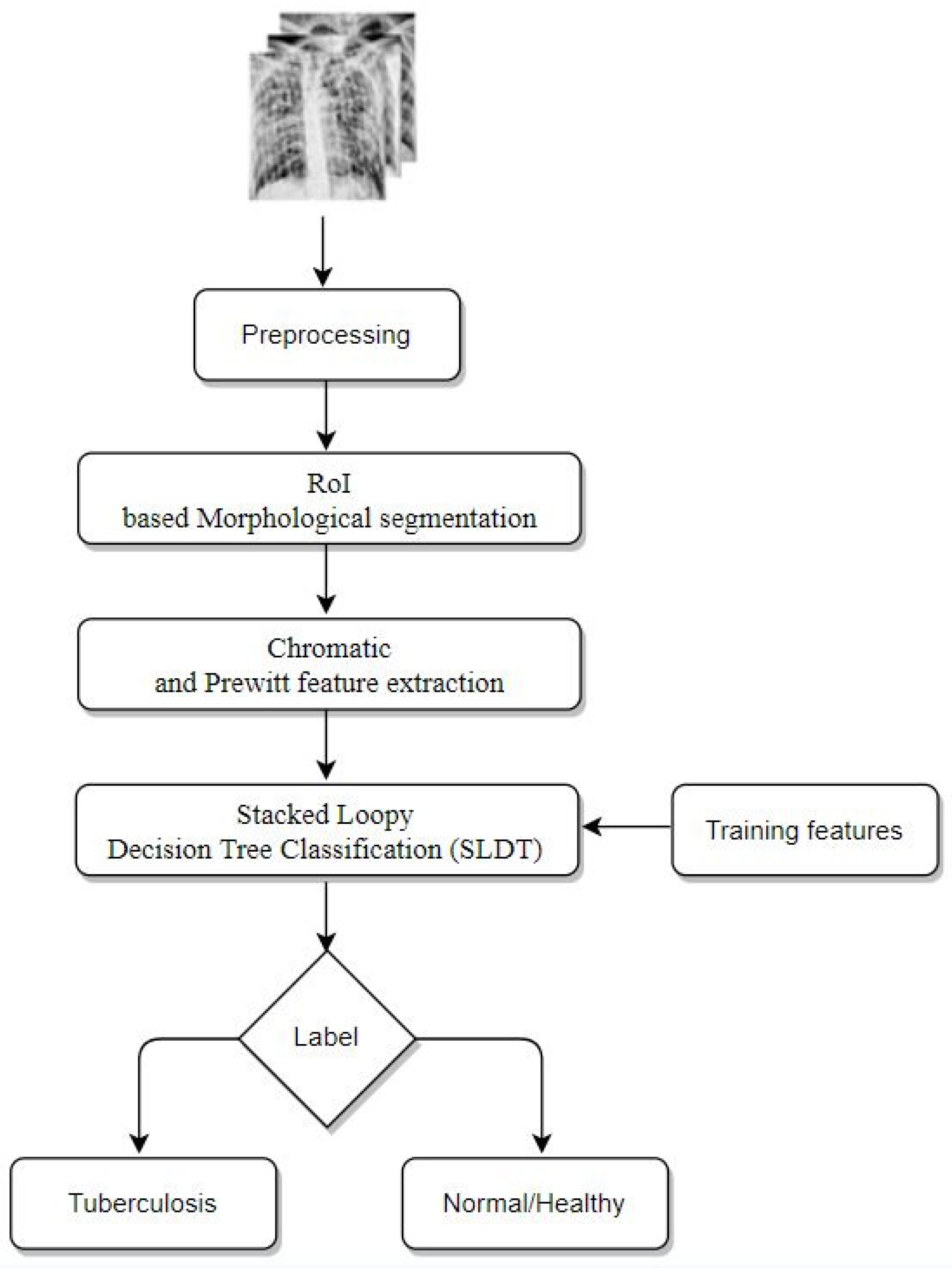
6. Methodology

In a three-stage approach, the proposed method identifies TB: segmentation, feature extraction, and classification. Noise reduction was applied to CXRs in order to detect and remove impulse abnormalities. The features were retrieved from the CXRs, and then the SLDT classifier was used to train the model and classify the dataset. The training and testing data were divided in the ratio of 70:30, and the ROI-based morphological method was used for segmentation. A block diagram of the proposed method is shown in Figure 1.

In Figure 1, the input images are CXR images in JPEG format. The image to be processed must be chosen by the user from its directory using the file name. After choosing the image to be analyzed, the ROI-based morphological segmentation will follow, then the chromatic and Prewitt feature extraction. The SLDT was used in training the features, and after the whole process had been undertaken, the labels were returned as either Tuberculosis or Normal.

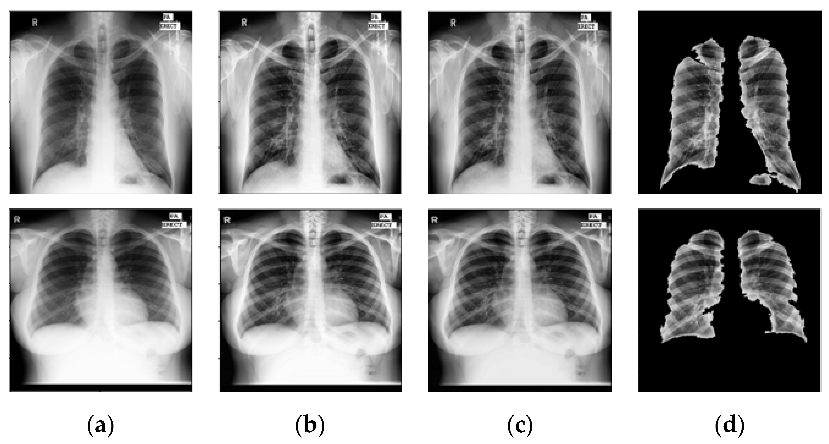
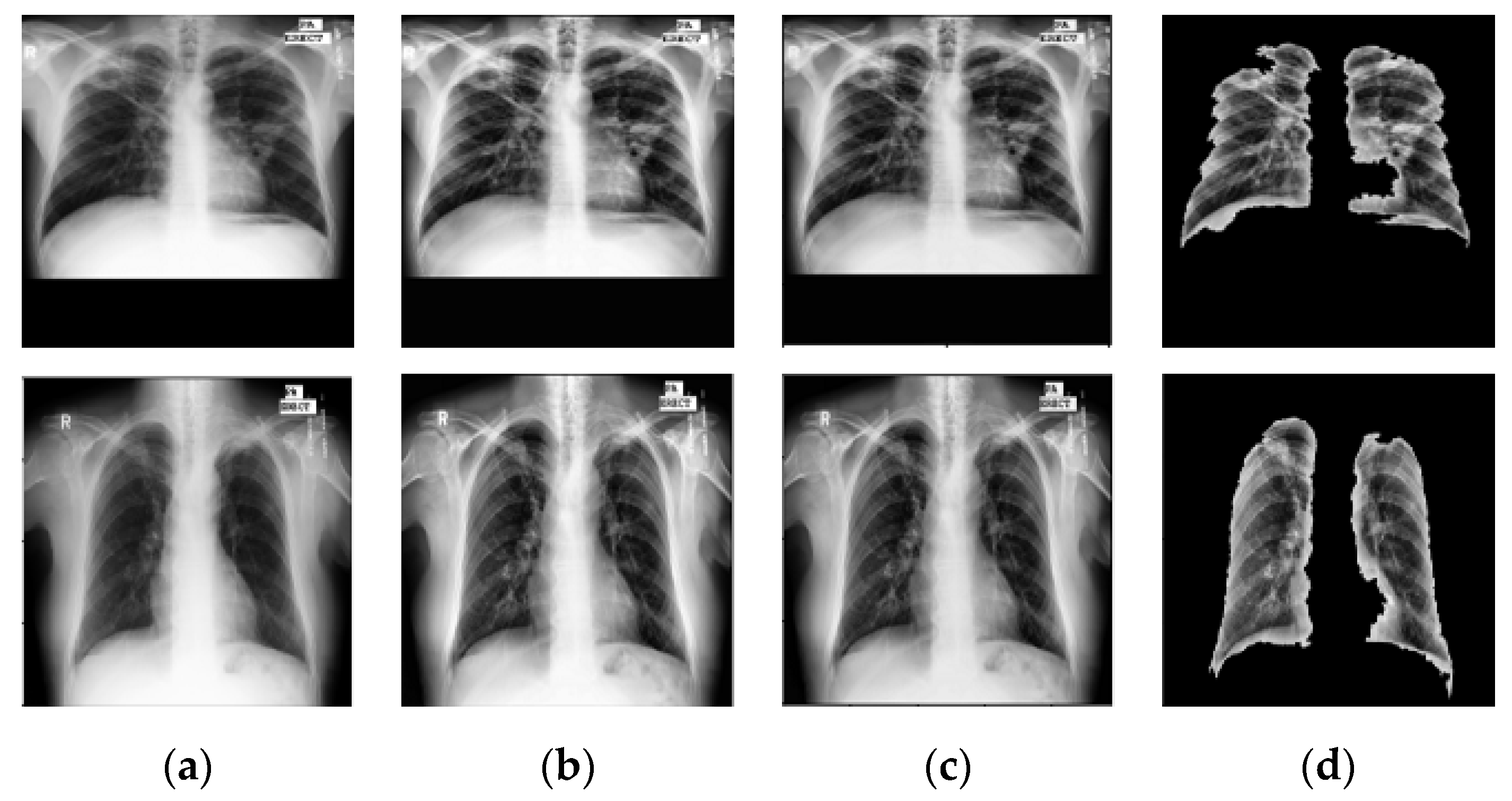
6.1. Weiner Filtering

The RGB format of the input image was used then transformed to a grayscale image before being processed further. The Wiener filter with a mask size 7 × 7 was used to remove the noise from the CXRs because it is one of the best methods to remove noise from CXRs, which often contain artifacts or noise due to patient movement.

For images with additive noise and blurring, the Wiener filter is the MSE-optimal stationary linear filter. The Wiener filter is calculated assuming second-order stationary signal and noise processes (in the random process sense) [22]. An observed image or degraded images can often be modeled as

$$x\left(i,j\right)=\iint h\left(i-i^{\prime },j-j^{\prime }\right) s\left(i^{\prime },j^{\prime }\right) d{i}^{\prime }d{j}^{\prime }+n\left(i,j\right)$$

(1)

where h is the imaging system’s point spread function, and n is the additive noise. We estimated the original images from the degraded image x in this case for image restoration.

$$x\left(i,j\right)=h\left(i,j\right) \times s\left(i,j\right)$$

(2)

where $h\left(i,j\right)$ is considered as the filter of the degraded image; $s\left(i,j\right)$ is considered as the original image; and $x\left(i,j\right)$ is considered as the modified or degraded image.

Hence, from Equations (1) and (2), we can derive the following generative model.

$$x\left(i,j\right)=h\left(i,j\right) \times s\left(i,j\right)\leftrightarrow X\left(a,b\right)=H\left(a,b\right) \times S\left(a,b\right)+N\left(a,b\right)$$

(3)

and for the moment, we ignore $n\left(i,j\right).$

Wiener filters are typically used in the frequency domain. Given a degraded image $x\left(i,j\right)$, the discrete Fourier transform (DFT) is used to produce $X \left(a,b\right)$. The original image spectrum is reconstructed by taking the product of $X\left(a,b\right)$ and the Wiener Filter $G\left(a,b\right)$.

$$\widehat{S}\left(a,b\right)=G\left(a,b\right)·X\left(a,b\right)$$

(4)

where $X\left(a,b\right)$ is DFT of $x\left(i,j\right)$.

$$\begin{array}{c}G\left(a,b\right) \mathrm{is} \mathrm{Weiner} \mathrm{Filter}\hfill \\ \widehat{S}\left(a,b\right) \mathrm{is} \mathrm{filtered} \mathrm{or} \mathrm{degraded} \mathrm{image}.\hfill \end{array}$$

The following Equation (5) will define the Wiener Filter.

$$G\left(a,b\right)=H\ast \left(a,b\right) Ps\left(a,b\right)/{\left|H\left(a,b\right)\right|}^2 Ps\left(a,b\right)+Pn\left(a,b\right)$$

(5)

where $Ps\left(u,v\right)$ is considered as the signal process by taking the Fourier transform of the signal autocorrelation. $Pn\left(u,v\right)$ is considered as a noise process by taking the Fourier transform of the signal autocorrelation.

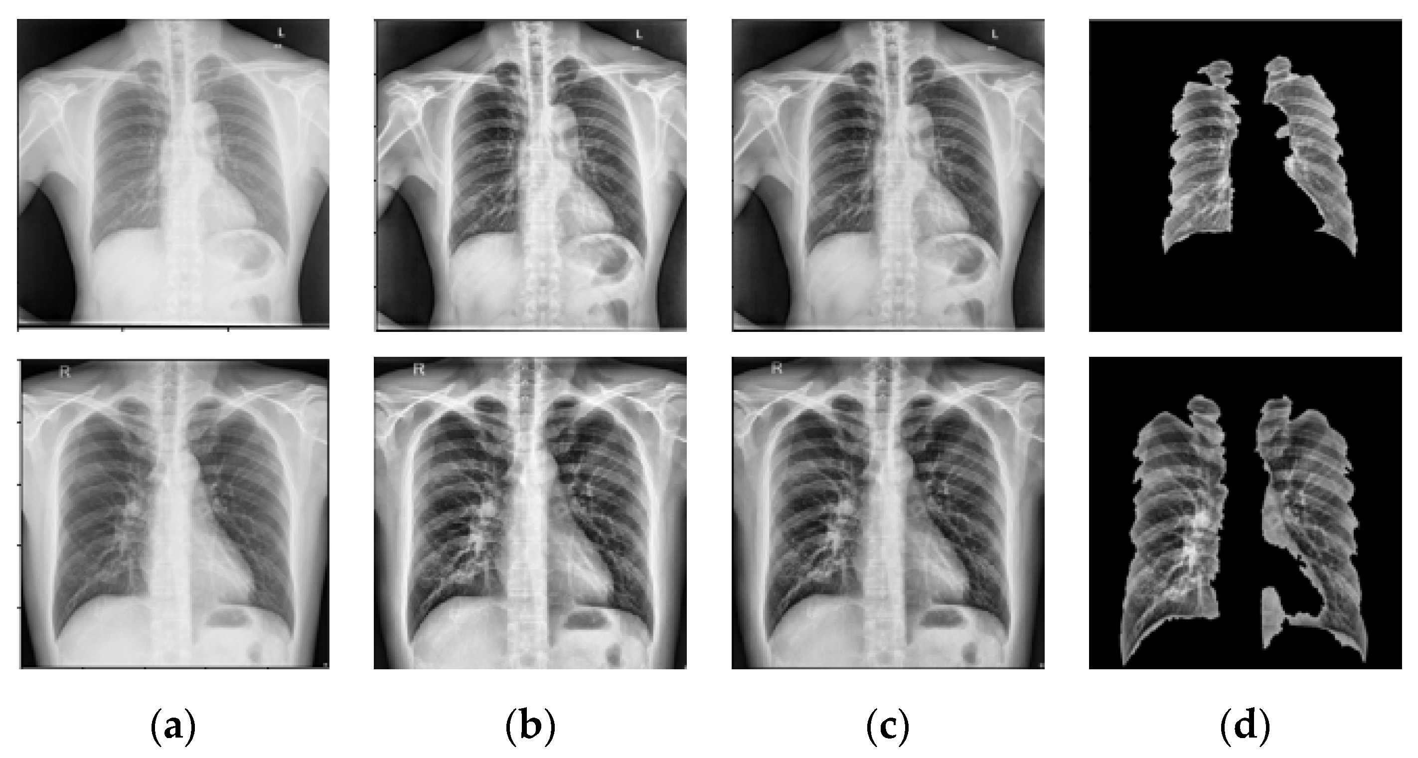
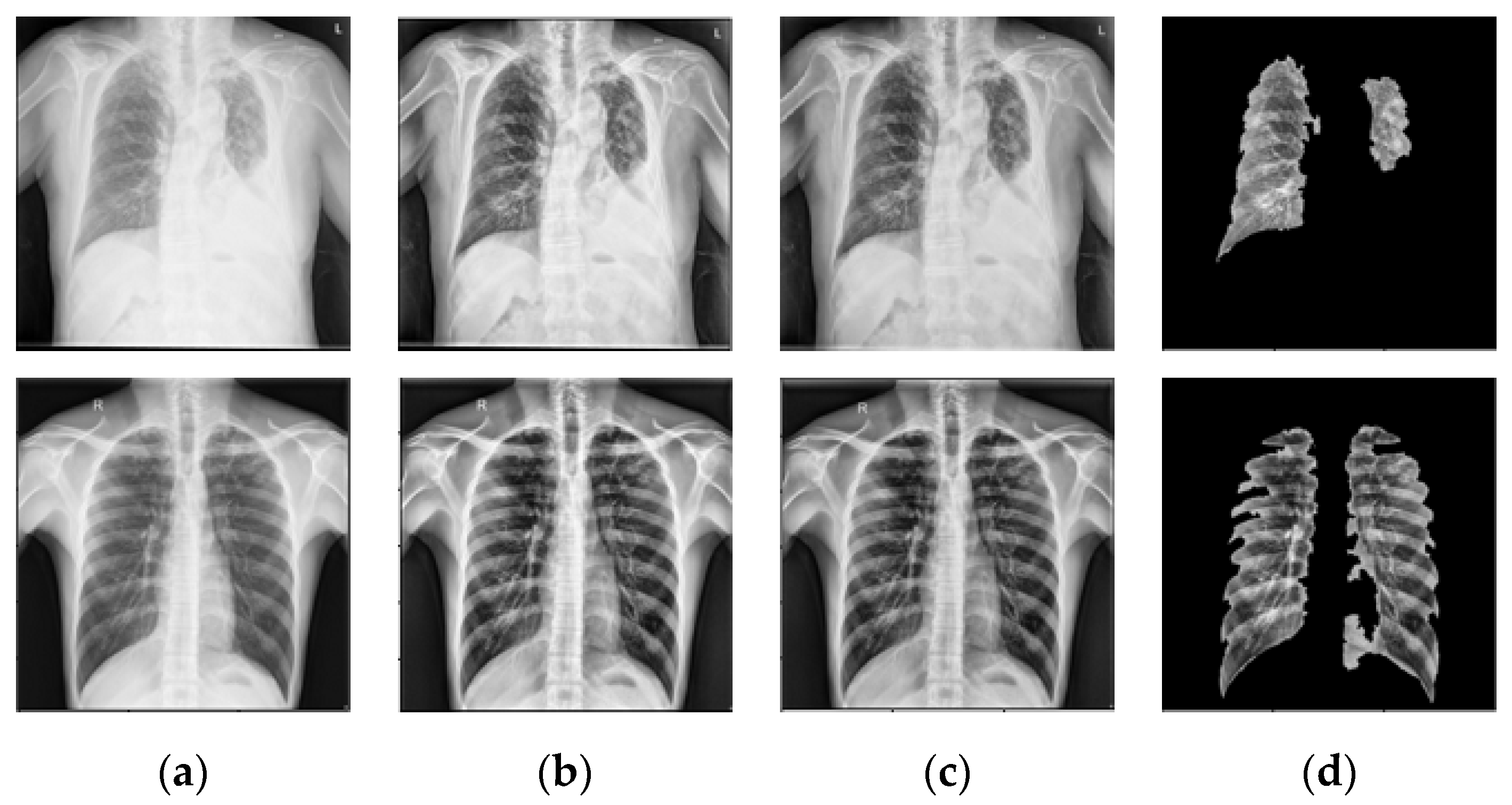
6.2. Prior TB Segmentation

Weiner Filter was used to remove unwanted noise from the CXRs, which can increase the image intensity uniformity while maintaining the texture and limits. A morphological-based region of interest (RoI) algorithm must then be used to remove the extra brain tissues. For automatic tracking of the location of the TB location, morphological operation was performed by the Weiner Filter and produced a mask that can be used for future segmentations. This method makes use of an image that combines morphological operations such as extended minima and morphological gradient algorithms to segment grayscale images of any size (8, 16, and 32-bit) in 2D and 3D.

Despite the fact that morphological operations are based on set theory, many of them are logical and simple to perform. The two most fundamental morphological activities are erosion and dilation. Several morphological operations have been represented as combinations of erosion, dilation, and simple set-theoretic operations such as the complement of a binary image. These were mentioned in Equations (6)–(9).

$$\{\begin{array}{c}{f}^c\left(A,B\right)=1, if f\left(A,B\right)=0\\ f^c\left(A,B\right)=0, if f\left(A,B\right)=1\end{array}$$

(6)

The intersection, $h=f\cap g$, of two binary images $f$ and $g$:

$$\begin{gathered} h\left(A,B\right)=1, if f\left(A,B\right)=1 \\ g\left(A,B\right)=1, and h\left(A,B\right)=0 otherwise \end{gathered}$$

(7)

and the union $h=f\cup g$ of two binary images $f$ and $g$:

$$\begin{gathered} h\left(A,B\right)=1, if f\left(A,B\right)=1 or g\left(A,B\right)=1, \\ and h\left(A,B\right)=0 otherwise \end{gathered}$$

(8)

The opening of an image $f$ by a structuring element $s$ (denoted by $f\circ s$) is an erosion followed by a dilation:

$$f\circ s=\left(f\ominus s\right)\oplus s$$

(9)

After selecting the RoI, morphological operation was applied to segment the image using the above equations.

6.3. Feature Extraction Phase

One of the most significant modules for classification is feature extraction. In this case, extracted features play a critical role in improving TB detection accuracy. The classifier was fed both chromatic and edge characteristics in this study.

The following steps are involved in extracting chromatic features:

(1)

Converting the RGB image to HSV image;

(2)

Determining the hue plane’s variance;

(3)

Calculating the hue plane’s standard deviation;

(4)

Determining the hue plane’s skewness;

(5)

Applying the above steps for the saturation and value; and

(6)

Combine all of these characteristics.

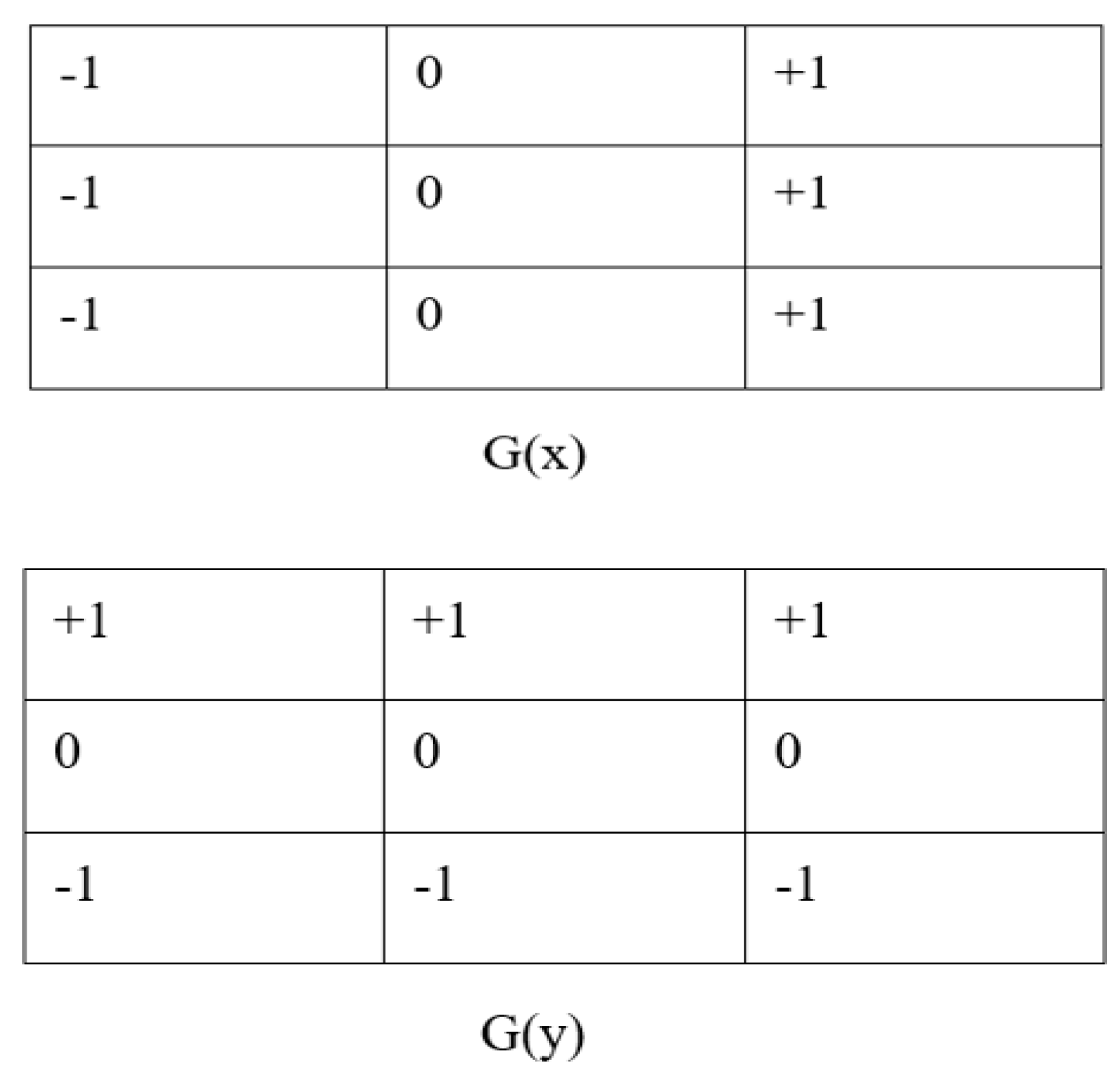
6.4. Prewitt Edge Detection

The Prewitt operator returns either the matching gradient vector or the vector’s normal, and is also used to measure the gradient intensity. The Prewitt operator works by performing convolution to the picture in the horizontal (x) and vertical (y) directions with a tiny, separable, integer-valued filter, which is a cheap and effective method for detecting edges. This method is only good for images that are not noisy and have a lot of contrast [23]. The spectral response is the difference between the Prewitt and Sobel operators, which is an effective way to figure out how big an edge is and how it is positioned.

Kernel $G\left(x\right)$ is used to calculate the vertical edge component, while Kernel $G\left(y\right)$ is used to compute the horizontal edge component (y) [24]. The gradient intensity in the current pixel is indicated by $\left|G\left(x\right)\right|+\left|G\left(y\right)\right|$. In order to find the absolute magnitude of gradient at each point and orientation of that gradient, we need to combine it together. Figure 2 shows the Prewitt operator, which is made up of a pair of $3\times 3$ convolution kernels.

The Kernels can be applied individually to the input image to provide independent gradient component measurements in each orientation (call these $Gx$ and $Gy$). Magnitude can be calculated by following Equations (10) and (11),

$$\left|\nabla f\right|=\sqrt{G{x}^2}+\sqrt{G{y}^2}$$

(10)

$$\left|\nabla f\right|=\left|G{x}^2\right|+\left|G{y}^2\right|$$

(11)

$$\begin{gathered} \nabla f-Magitude of image \\ Gx-gradient along x direction \\ Gy-gradient along y direction \end{gathered}$$

Angle of computation of the gradient of a picture is based on finding the partial derivatives of $\partial f/\partial x$ and $\partial f/\partial y$ at each pixel position by Equation (12). These derivatives can be applied to a whole image using masks with the size $3\times 3$ and the convolution method.

$$Angle of \nabla f={\tan }^{-1}(\frac{G\left(x\right)}{G\left(y\right)})$$

(12)

Based on Equation (14), the image’s magnitude values and angles of Prewitt convolutional kernels are used to implement the central point by following Equations (13) and (14).

$$Gx=\left(z7+z8+z9\right)-\left(z1+z2+z3\right)$$

(13)

$$Gy=\left(z5+z6+z9\right)-\left(z1+z4+z7\right)$$

(14)

6.5. Stacked Loopy Decision Tree (SLDT) Algorithm

Stacking is a machine learning ensemble algorithm that is also known as stacked generalization. Using a meta-learning method, it learns how to merge predictions from two or more underlying machine learning algorithms. Stacking provides the advantage of combining the capabilities of a number of high-performing models to produce predictions that are better than any one model in the ensemble on a classification or regression problem. Algorithm 1 will explain the proposed system.

The architecture of the stacking model consists of two or more base models (known as level-0 models) and a meta-model (known as levels-1) that integrates the predictions of the base models.

(1)

Level 0 models (base models) are used to compile and adapt to training data, whereas Level 1 models (Meta Mode) are used to integrate the basic model predictions to the greatest extent possible;

(2)

Strategies to access primary models such as training data entry can also be included in meta-training models on how to best combine design elements;

(3)

Once the meta-training model’s dataset has been generated, the meta-model can be trained independently on it, while the base models can be trained on the complete original training dataset;

(4)

The ultimate conclusion is reached using a decision tree, which is iterated for numerous loops to forecast the image’s label; and

(5)

Generally, a decision tree algorithm has a decision node and leaf node. Several branches can be made by using the decision nodes. At same time, decision output is represented by the leaf nodes without multiple branches.

Algorithm 1. Proposed Algorithm.

Input: Image Output: Optimized Image 1. Read input image. 2. Transform the image to a gray image. 3. Use Equation (1) to apply the Weiner Filter. 4. Carry out segmentation by Equation (5). 5. Extract chromatic features for images in the data set by Prewitt edge. 6. Train the dataset and make the decision using SLDT.

7. Experimental Results

Evaluation Metrics

The number of correct predictions of healthy and TB patients was used to determine the SLDT performance. The following performance criteria were utilized to evaluate: accuracy, sensitivity, specificity, and area under curve (AUC). These variables are expressed in Equations (15)–(17) below.

$$Sensitivity(\%)=TP/TP+FN\times 100$$

(15)

$$Specificity(\%)=TN/FP+TN\times 100$$

(16)

$$Accuracy(\%)=\left(TP+TN\right)/TP+FN+TN+FP\times 100$$

(17)

where TP, TN, FN, and FP are True Positive, True Negative, False Negative, and False Positive, respectively.

The results of several phases performed on the normal and abnormal images of TB CXRs were illustrated by various datasets such as MC and CHN, which are shown in Figure 3, Figure 4, Figure 5 and Figure 6, respectively.

Figure 3 was processed and taken from normal images of the CHN dataset.

In Figure 3, the first column (a) illustrates the input image, which is an normal CXR image; the second column (b) illustrates the output image, which was equalized from the given normal input image; the third column (c) illustrates the Weiner Filtered image of the given input image; and the fourth column (d) illustrates the output image, which was segmented using ROI-based morphological operations. It can be noted that column d is segmented, which is output from the first column (a), second column (b), and third column (c). We could observe different between original images and segmented images using our proposed system. The above experiment was processed on a CHN normal dataset.

Figure 4 was processed and taken from abnormal images of the CHN dataset.

In Figure 4, the first column (a) illustrates the input image, which is the abnormal CXR image; the second column (b) illustrates the output image, which was equalized from the given abnormal input image; the third column (c) illustrates the Weiner Filtered image of the given input image; and the fourth column (d) illustrates the output image, which was segmented using ROI-based morphological operations. The above experimental results were processed and taken from abnormal dataset of CHN.

Figure 5 was taken from normal images of the MC dataset.

In Figure 5, the first column (a) illustrates the input image, which is the normal CXR image; the second column (b) illustrates the output image, which was equalized from the given normal input image; the third column (c) illustrates the Weiner Filtered image of the given input image; and the fourth column (d) illustrates the output image, which was segmented using ROI-based morphological operations. These images were taken from the MC normal dataset.

Figure 6 was processed and taken from abnormal images of the MC dataset.

In Figure 6, the first column (a) illustrates the input image, which is the abnormal CXR image; the second column (b) illustrates the output image, which was equalized from the given abnormal input image; the third column (c) illustrates the Weiner Filtered image of the given input image; and the fourth column (d) illustrates the output image, which was segmented using ROI-based morphological operations. The above experimental results were processed and taken from the abnormal dataset of MC.

The performance metrics, which were evaluated using the formulas that were given above and its comparison with the existing systems with the proposed system, were displayed in

Table 1. Performance measures of the proposed method with the existing method by the CHN dataset.

Authors	Methods	Dataset	Accuracy	Sensitivity	Specificity	AUC
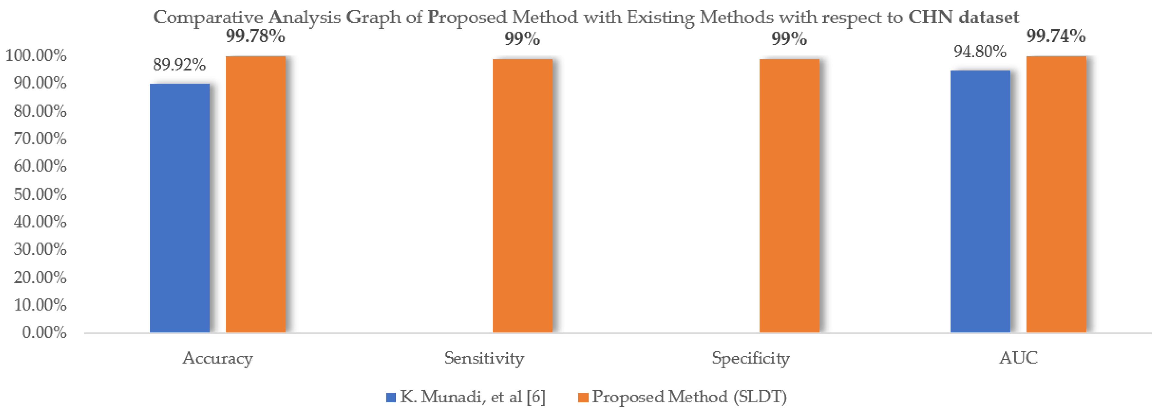
K. Munadi et al. [9]	CNN with Transfer learning	CHN	89.92%	N/A	N/A	94.8%
Proposed Method	SLDT	CHN	99.78%	99%	99%	99.74%

,

Table 2. Performance measures of the proposed method with the existing methods by the MC dataset.

Authors	Methods	Dataset	Accuracy	Sensitivity	Specificity	AUC
Rajaraman and Antari [15]	Ensemble Method	MC	94.1%	N/A	N/A	99%
S. Jaeger et al. [16]	Graph cut	MC	84%	N/A	N/A	90%
Hwang et al. [17]	CNN with Transfer learning	MC	83.7%	N/A	N/A	92.6%
Proposed Method	SLDT	MC	98.9%	98%	97.3%	99%

,

Table 3. Performance measures of the proposed method with existing methods by the combined dataset 1 (MC and CHN).

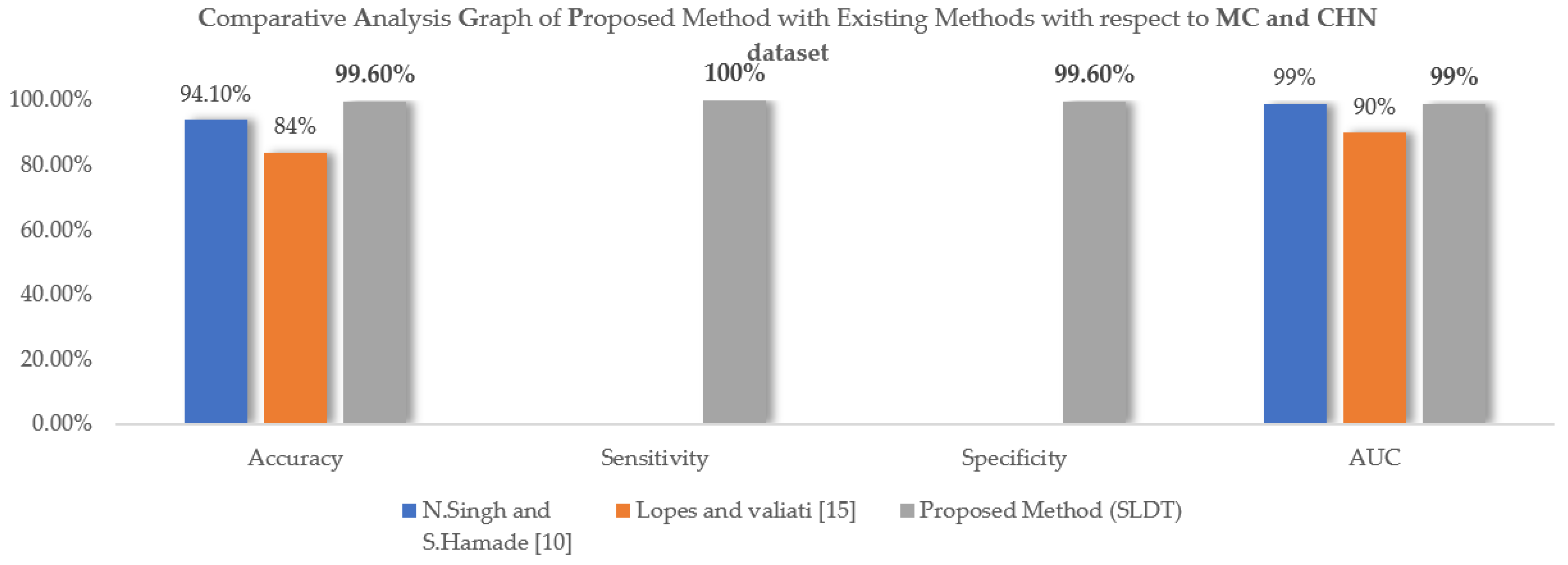
Authors	Methods	Dataset	Accuracy	Sensitivity	Specificity	AUC
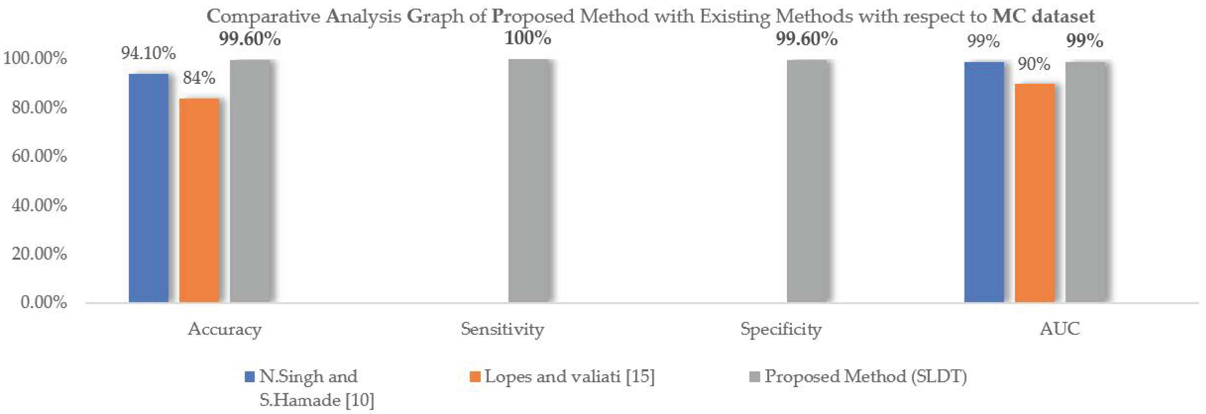
N. Singh and S. Hamade [13]	SVM	MC and CHN	N/A	N/A	100%	96%
Lopes and Valiati [18]	CNN with Transfer learning	MC and CHN	84.7%	N/A	N/A	92.6%
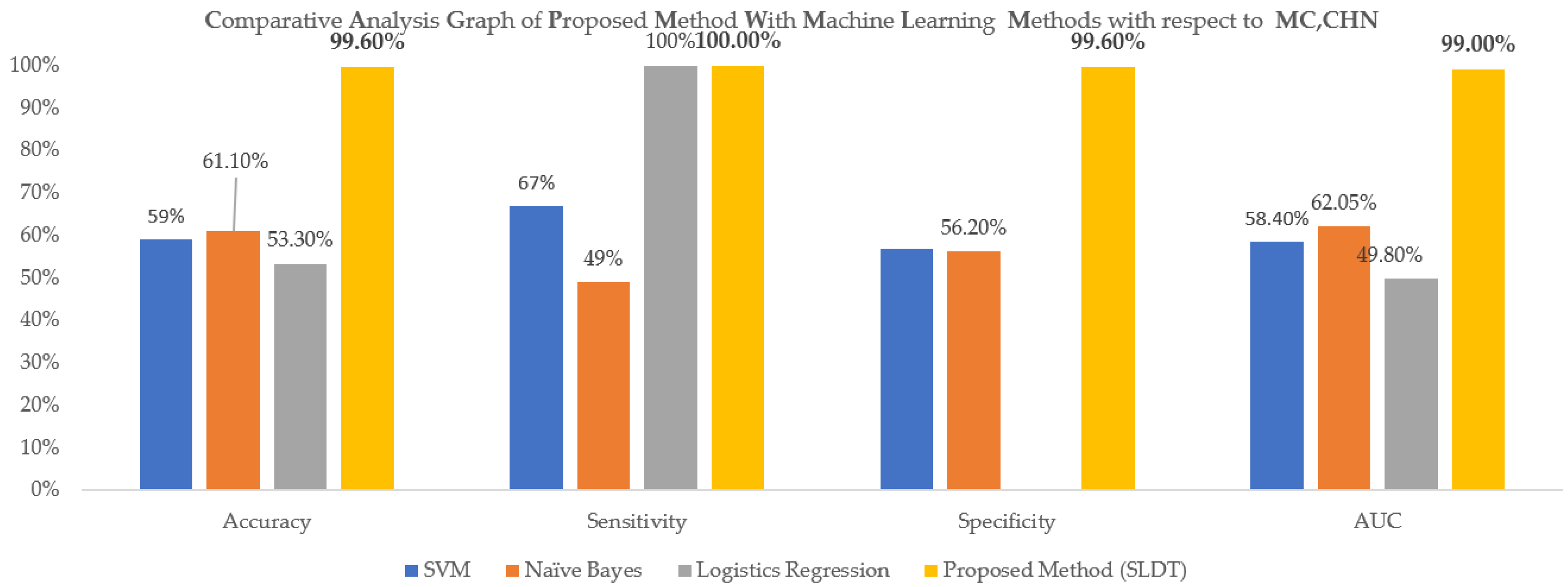
Proposed Method	SLDT	MC and CHN	99.6%	100%	99.6%	99%

and

Table 4. Performance measures of the proposed method with existing methods by combined dataset 2 (NLM, Belarus and RSNA).

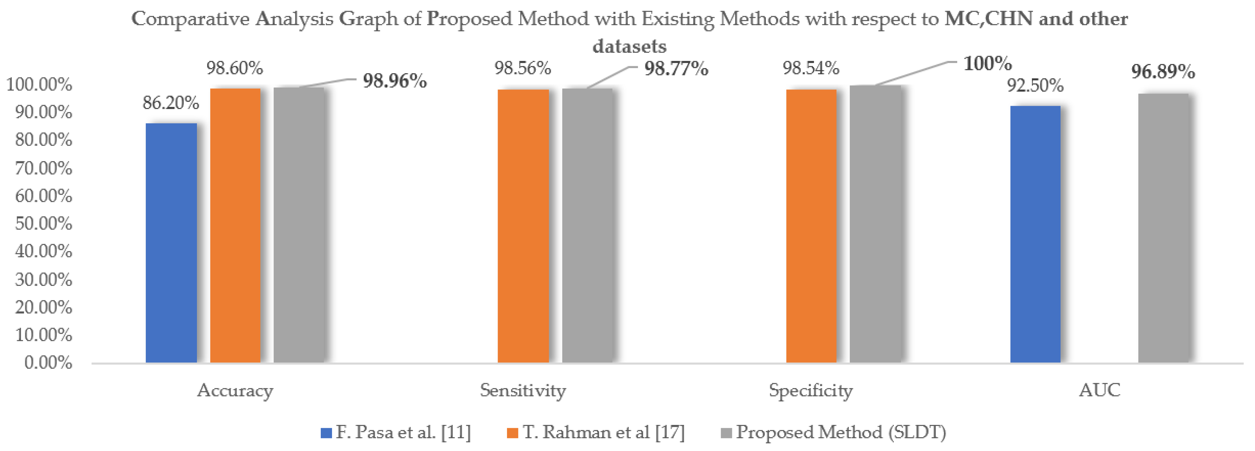
Authors	Methods	Dataset	Accuracy	Sensitivity	Specificity	AUC
F. Pasa et al. [14]	Optimized CNN	MC, CHN and Belarus	86.2%	N/A	N/A	92.5%
T. Rahman et al. [20]	CNN with Transfer learning	NLM (MC and CHN), Belarus, NIAID TB portal and RSNA	98.6%	98.56%	98.54%	N/A
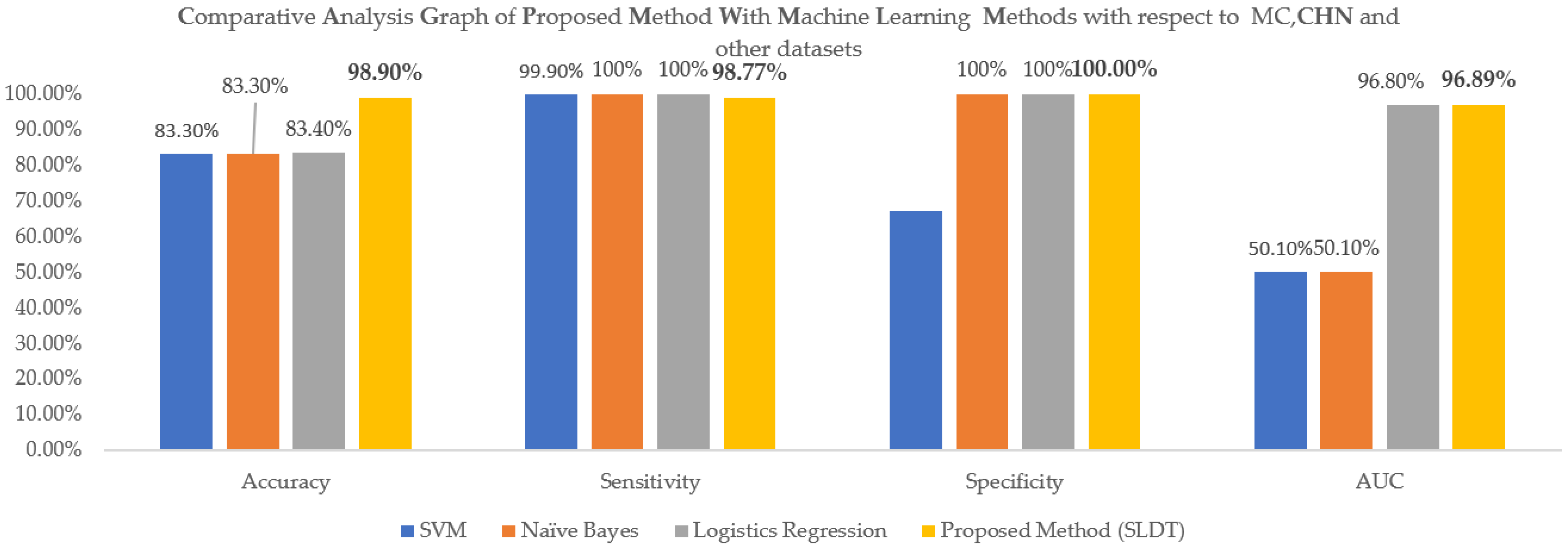
Proposed Method	SLDT	NLM (MC and CHN), Belarus and RSNA	98.96%	98.77%	100%	96.89%

with respect to the CHN, MC, combined datasets 1 (MC and CHN) and the other combined datasets 2 (NLM, Belarus, and RSNA).

In Table 1, the accuracy, sensitivity, specificity, and AUC scores are displayed. These are the major performance measures of the proposed method used to compare the performance to the existing method. Both methods used the CHN dataset. Table 2 presents the performance measures of the existing methods and the proposed method with the MC dataset.

In Table 2, we compared the performance measures of accuracy, sensitivity, specificity, and AUC with existing methods by the same dataset such as MC. The proposed method attained the highest accuracy rate among the existing methods. Moreover, the sensitivity, specificity, and AUC scores were presented. The performance measures of the proposed method with existing methods in the combined dataset 1 (MC and CHN) is presented in Table 3.

In Table 3, existing methods and the proposed method’s performance were compared with its performance in the combined dataset 1 such as MC and CHN. The proposed method obtained the highest accuracy, sensitivity, specificity, and AUC scores. The performance measures of the proposed method with existing methods by the combined dataset 2 (NLM, Belarus and RSNA) is presented in Table 4.

In Table 4, the proposed method was analyzed by comparing various performance measures with the existing methods using combined dataset 2 (NLM, Belarus and RSNA). The proposed method was still the highest performer among the existing methods.

Table 5. Performance measures of the proposed method with other machine learning methods by the CHN dataset.

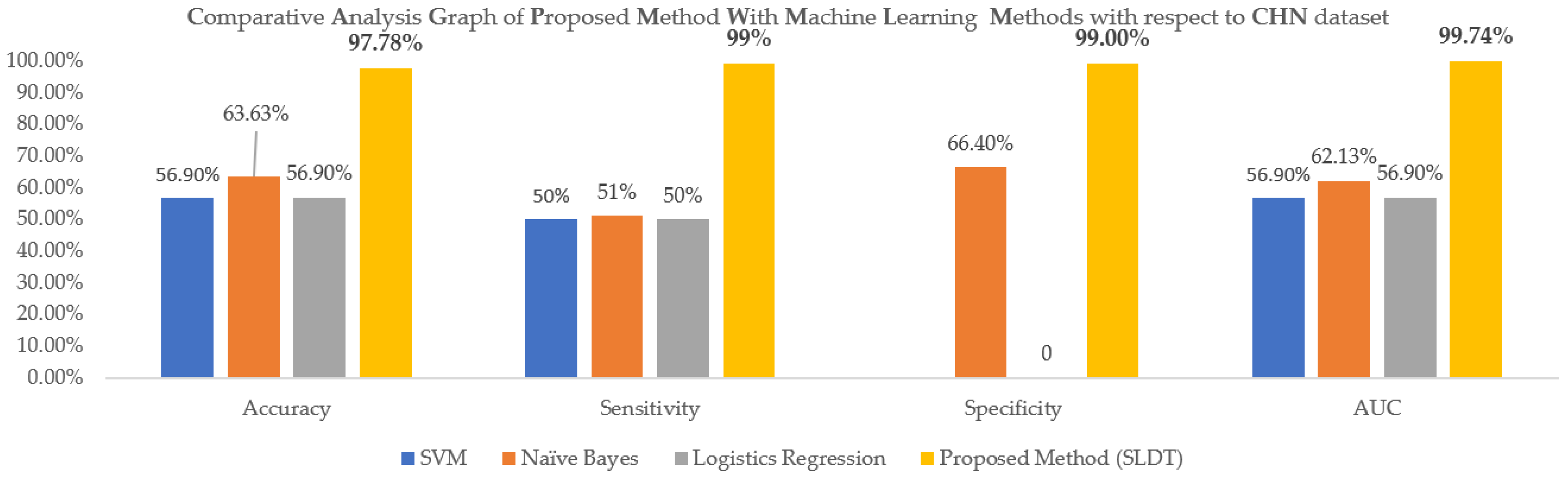
Methods	Accuracy	Sensitivity	Specificity	AUC
SVM	56.9%	50%	N/A	56.9%
Naïve Bayes	63.63%	51%	66.4%	62.13%
Logistic Regression	56.9%	50%	N/A	56.9%
SLDT	99.78%	99%	99%	99.74%

,

Table 6. Performance measures of the proposed method with other machine learning methods by the MC dataset.

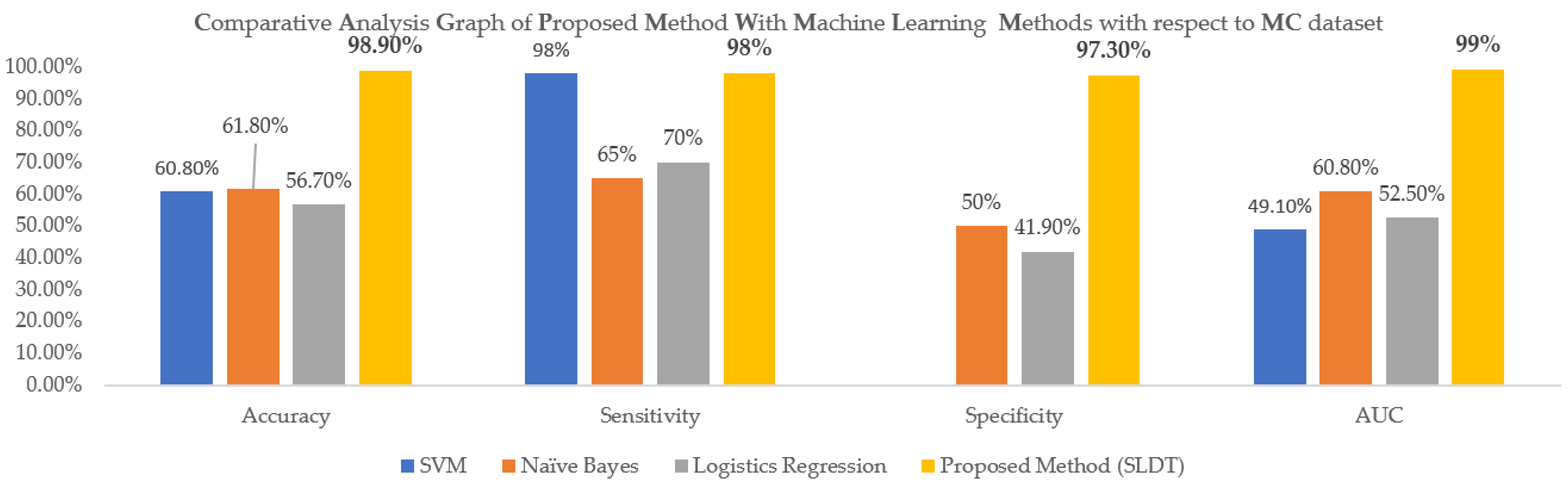
Methods	Accuracy	Sensitivity	Specificity	AUC
SVM	60.8%	98%	N/A	49.1%
Naive Bayes	61.8%	65%	50%	60.8%
Logistic Regression	56.70%	70%	41.9%	52.5%
SLDT	98.9%	98%	97.3%	99%

,

Table 7. Performance measures of the proposed method with other machine learning methods in combined dataset 1 (MC and CHN).

Methods	Accuracy	Sensitivity	Specificity	AUC
SVM	59%	67%	56.7%	58.4%
Naïve Bayes	61.1%	49%	56.2%	62.05%
Logistic Regression	53.3%	100%	N/A	49.8%
SLDT	99.6%	100%	99.6%	99%

and

Table 8. Performance measures of the proposed method with other machine learning methods in the combined dataset 2 including NLM, Belarus, and RSNA.

Methods	Accuracy	Sensitivity	Specificity	AUC
SVM	83.3%	99.9%	67%	50.1%
Naïve Bayes	83.3%	100%	100%	50.1%
Logistic Regression	83.4%	100%	100%	96.8%
SLDT	98.9%	98.77%	100%	96.89%

show the proposed method’s performance compared with other machine learning algorithms with respect to the following datasets: CHN, MC, combined dataset 1 (MC and CHN) and combined dataset 2 (NLM, Belarus, and RSNA).

In Table 5, the proposed method was compared with other machine learning methods such as support vector machine (SVM), naïve Bayes, and logistic regression. Results show that the proposed methods had better performance measures among other machine learning algorithms using the CHN dataset. The performance measures of the proposed method with other machine learning methods in the MC dataset is shown in Table 6.

In Table 6, it can be seen that the proposed method had the highest performance in accuracy, sensitivity, specificity, and AUC among the other machine learning algorithms using the same dataset, the MC dataset. The performance measures of the proposed method with other machine learning methods in combined dataset 1 (MC and CHN) are displayed in Table 7.

In Table 7, the proposed method was compared with other machine learning algorithms with respect to the combined dataset 1, which includes the MC and CHN datasets. The proposed method had the highest performance, showing 99.6% accuracy and 99% AUC compared with SVM, naïve Bayes, and logistic regression. Finally, the performance measures of the proposed method with other machine learning methods in the combined dataset 2 including NLM, Belarus, and RSNA are displayed in Table 8.

Figure 7, Figure 8, Figure 9 and Figure 10 show the visual representation of the comparative analysis of the proposed methods with the existing methods with respect to the various datasets used in the experiments including CHN, MC, and the combined dataset 1 (MC and CHN) and the other combined dataset 2 (NLM, Belarus, and RSNA).

Figure 11, Figure 12, Figure 13 and Figure 14 show the visual representation of the comparative analysis of the proposed method with various machine learning methods with respect to the various datasets used in the experiments.

According to the various datasets, CHN, MC, combined dataset 1 (MC and CHN), and the other combined dataset 2 (NLM, Belarus, and RSNA), we analyzed, processed, and finally obtained some experimental results by comparing the performance measures with the proposed method. From the above experimental results, our proposed method obtained some significant improvements and achieved the highest performance among other existing methods.

8. Conclusions

In this article, a ROI-based morphological segmentation method and feature extraction and segmentation for tuberculosis CXR images were proposed. The experimental results showed that using the proposed system (SLDT), tuberculosis could be accurately predicted in CXR according to the various datasets. Another benefit of the proposed methodology is that it is completely automated, requiring minimal user intervention, which is important when dealing with massive amounts of data. Future studies can also include COVID-19 and other datasets to detect and predict the segmentation of impacted regions for additional investigations. Future researchers in this field can explore ways to improve the accuracy of the 3D image segmentation.

References

- Major Infectious Diseases. Available online: https://www.ncbi.nlm.nih.gov/books/NBK525174/ (accessed on 6 May 2021).
- Karargyris, A.; Siegelman, J.; Tzortzis, D.; Jaeger, S.; Candemir, S.; Xue, Z.; Santosh, K.C.; Vajda, S.; Antani, S.; Folio, L.; et al. Combination of texture and shape features to detect pulmonary abnormalities in digital chest X-rays. Int. J. Comput. Assist. Radiol. Surg. 2016, 11, 99–106. [Google Scholar] [CrossRef] [PubMed]
- Hogeweg, L.; Sánchez, C.I.; Maduskar, P.; Philipsen, R.; Story, A.; Dawson, R.; Theron, G.; Dheda, K.; Peters-Bax, L.; van Ginneken, B. Automatic Detection of Tuberculosis in Chest Radiographs Using a Combination of Textural, Focal, and Shape Abnormality Analysis. IEEE Trans. Med Imaging 2015, 34, 2429–2442. [Google Scholar] [CrossRef] [PubMed]
- World Health Organization. Global Tuberculosis Report. 2018. Available online: https://apps.who.int/iris/handle/10665/274453, (accessed on 6 May 2021).
- Sputum Testing for Tuberculosis (TB). Available online: https://www.healthlinkbc.ca/healthlinkbc-files/sputum-tuberculosis-testing (accessed on 6 May 2021).
- Interferon Gamma Release Assay Test (IGRA Test). Available online: https://www.health.nsw.gov.au/Infectious/tuberculosis/Pages/interferon-gamma-release-assay-test.aspx (accessed on 6 May 2021).
- Chen, X.; Sa, J.; Li, M.; Zhou, Y. Combined prediction model of tuberculosis based on generalized regression neural network. In Proceedings of the 2020 IEEE International Conference on Artificial Intelligence and Computer Applications (ICAICA), Dalian, China, 27–29 June 2020; pp. 577–581. [Google Scholar]
- Zaman, A.; Khattak, S.S.; Hassan, Z. Medical Imaging for the Detection of Tuberculosis Using Chest Radio Graphs. In Proceedings of the 2019 International Conference on Advances in the Emerging Computing Technologies (AECT), Al Madinah Al Munawwarah, Saudi Arabia, 10 February 2020; pp. 1–5. [Google Scholar]
- Munadi, K.; Muchtar, K.; Maulina, N.; Pradhan, B. Image enhancement for tuberculosis detection using deep learning. IEEE Access 2020, 8, 217897–217907. [Google Scholar] [CrossRef]
- Fariza, A.; Mu’arifin; Puspitasari, A. Spatial Fuzzy Risk Mapping for Tuberculosis in Surabaya, Indonesia. In Proceedings of the 2020 International Electronics Symposium (IES), Surabaya, Indonesia, 29–30 September 2020; pp. 613–619. [Google Scholar]
- Serrão, M.K.M.; Costa, M.G.F.; Fujimoto, L.B.; Ogusku, M.M.; Filho, C.F.F.C. Automatic Bacillus Detection in Light Field Microscopy Images Using Convolutional Neural Networks and Mosaic Imaging Approach. In Proceedings of the 2020 42nd Annual International Conference of the IEEE Engineering in Medicine & Biology Society (EMBC), Montreal, QC, Canada, 20–24 July 2020; pp. 1903–1906. [Google Scholar]
- Cao, Y.; Mao, J.; Yu, H.; Zhang, Q.; Wang, H.; Zhang, Q.; Guo, L.; Gao, F. A Novel Hybrid Active Contour Model for Intracranial Tuberculosis MRI Segmentation Applications. IEEE Access 2020, 8, 149569–149585. [Google Scholar] [CrossRef]
- Singh, N.; Hamde, S. Tuberculosis Detection Using Shape and Texture Features of Chest X-rays. In Innovations in Electronics and Communication Engineering; Saini, H., Singh, R., Kumar, G., Rather, G., Santhi, K., Eds.; Lecture Notes in Networks and Systems; Springer: Singapore, 2019; Volume 65. [Google Scholar] [CrossRef]
- Pasa, F.; Golkov, V.; Pfeiffer, F.; Cremers, D.; Pfeiffer, D. Efficient deep network architectures for fast chest X-ray tuberculosis screening and visualization. Sci. Rep. 2019, 9, 19. [Google Scholar] [CrossRef] [PubMed] [Green Version]
- Rajaraman, S.; Antani, S.K. Modality-specific deep learning model ensembles toward improving TB detection in chest radiographs. IEEE Access 2020, 8, 27318–27326. [Google Scholar] [CrossRef] [PubMed]
- Jaeger, S.; Karargyris, A.; Candemir, S.; Folio, L.; Siegelman, J.; Callaghan, F.; Xue, Z.; Palaniappan, K.; Singh, R.K.; Antani, S.; et al. Automatic tuberculosis screening using chest radiographs. IEEE Trans. Med. Imaging 2014, 33, 233–245. [Google Scholar] [CrossRef] [PubMed]
- Hwang, S.; Kim, H.-E.; Kim, H.-J. A novel approach for tuberculosis screening based on deep convolutional neural networks. Proc. SPIE Med. Imaging 2016, 9785, 97852W. [Google Scholar]
- Lopes, U.K.; Valiati, J.F. Pre-trained convolutional neural networks as feature extractors for tuberculosis detection. Comput. Biol. Med. 2017, 89, 135–143. [Google Scholar] [CrossRef] [PubMed]
- Kwon, H. MedicalGuard: U-Net Model Robust against Adversarially Perturbed Images. Secur. Commun. Netw. 2021, 2021, 5595026. [Google Scholar] [CrossRef]
- Rahman, T.; Khandakar, A.; Kadir, M.A.; Islam, K.R.; Islam, K.F.; Mahbub, Z.B.; Ayari, M.A.; Chowdhury, M.E.H. Reliable Tuberculosis Detection Using Chest X-ray with Deep Learning, Segmentation and Visualization. IEEE Access. 2020, 8, 191586–191601. [Google Scholar] [CrossRef]
- Candemir, S.; Jaeger, S.; Palaniappan, K.; Musco, J.P.; Singh, R.K.; Xue, Z.; Karargyris, A.; Antani, S.; Thoma, G.; McDonald, C.J. Lung Segmentation in Chest Radiographs Using Anatomical Atlases with Nonrigid Registration. IEEE Trans. Med Imaging 2014, 33, 577–590. [Google Scholar] [CrossRef] [PubMed]
- The Wiener Filter. Available online: https://homepages.inf.ed.ac.uk/rbf/CVonline/LOCAL_COPIES/VELDHUIZEN/node15.html (accessed on 3 March 2021).
- Vijayarani, S.; Vinupriya, M. Performance Analysis of Canny and Sobel Edge Detection Algorithms in Image Mining. Int. J. Innov. Res. Comput. 2013, 1, 1760–1767. [Google Scholar]
- Prewitt Operator. Available online: https://en.wikipedia.org/wiki/Prewitt_operator (accessed on 3 March 2021).