Article

Joint Motion Planning of Industrial Robot Based on Modified Cubic Hermite Interpolation with Velocity Constraint

1
School of Mechanical Engineering, Northwestern Polytechnical University, Xi’an 710072, China
2
College of Engineering, Honghe University, Mengzi 661100, China
*
Authors to whom correspondence should be addressed.
Appl. Sci. 2021, 11(19), 8879; https://doi.org/10.3390/app11198879
Submission received: 6 September 2021 / Revised: 15 September 2021 / Accepted: 21 September 2021 / Published: 24 September 2021
(This article belongs to the Special Issue Advanced Robotics Applications in Industry)

Abstract

:

Featured Application

Industrial robot joint smooth movement via multiple positions with constrained velocities.

Abstract

As for industrial robots’ point-to-point joint motion planning with constrained velocity, cubic polynomial planning has the problem of discontinuous acceleration; quintic polynomial planning requires acceleration to be specified in advance, which will likely cause velocity to fluctuate largely because appropriate acceleration assigned in advance is hardly acquired. Aiming at these problems, a modified cubic Hermite interpolation for joint motion planning was proposed. In the proposed methodology, knots of cubic Hermite interpolation need to be reconfigured according to the initial knots. The formulas for how to build new knots were put forward after derivation. Using the newly-built knots instead of initial knots for cubic Hermite interpolation, joint motion planning was carried out. The purpose was that the joint planning not only satisfied the displacement and velocity constraints at the initial knots but also guaranteed C2 continuity and less velocity fluctuation. A study case was given to verify the rationality and effectiveness of the methodology. Compared with the other two planning methods, it proved that the raised problems can be solved effectively via the proposed methodology, which is beneficial to the working performance and service life of industrial robots.

1. Introduction

Industrial robots are widely used in handling, painting, welding, assembly, packaging and other fields. With the development of robot technology, industrial robots are gradually applied to polishing, monitoring, automatic manufacture system and so on [1,2]. The manipulator movements become more complex and need to satisfy higher working performances. Therefore, trajectory planning of industrial robots has to meet higher requirements. The most basic task of industrial robot motion planning is to meet the requirements for end-effector displacement and velocity [3]. Moreover, favorable trajectory planning should ensure smooth movements, fewer vibrations, impacts and mechanical wear so that it can improve working performance and extend service life [4].
Motion planning of industrial robots can be divided into two types: one is in the workspace for end-effector, the other is in joint space for joints. For motion planning in the workspace, the inverse kinematics function needs to be solved repeatedly to calculate angular displacements and angular velocities of joints, which requires a large amount of calculation [5]. Furthermore, end-effector singularity possibly appears and will make joints rotate incorrectly so that the end-effector cannot complete work successfully. For motion planning in joint space, only a few inverse kinematics solutions are needed to find out the angular displacements and angular velocities at several target points of joints. Therefore, motion planning in joint space can reduce inverse kinematics calculation largely so that computation efficiency is improved, and also can avoid joints singularity and redundancy [6]. As a result, motion planning in joint space is more suitable for the point-to-point (PTP) motion of industrial robots.
The main methods of joint motion planning are reviewed below. Linear planning with parabolic transition has the advantage that joint speed remains constant in the linear phase, but sufficient transition time must be ensured, and angular acceleration is not continuous. The widely used cubic polynomial planning has the advantages of simple principle and less computation. However, when it is used to multiple points with constrained velocities, the angular acceleration at the connection points is broken, which will lead to vibrations and impacts and make the robot arm tremble. Quintic polynomial planning has continuous angular acceleration. However, quintic polynomial interpolation requires specifying in advance the angular acceleration value of the joint at each target point. If it is not preset properly, the angular velocities will fluctuate back and forth, which is not conducive to joint motion control. Frustratingly, it is difficult to give appropriate angular acceleration values in advance [7]. In addition, quintic multinomial has a higher degree than cubic polynomial so that velocities and accelerations change more intensely, and larger velocity and acceleration peaks appear. B spline interpolation is also used in motion planning [8,9,10]. However, when the cubic B-spline curve is used for multiple points with constrained velocities, acceleration is not continuous at connecting points as well. Some researchers carried out lots of studies about cubic B spline and realized G2 continuity at the connecting knots [11,12]. However, G2 continuity refers to curvature continuity, and continuity of second-order derivative C2 is not fully achieved.
In order to solve the complicated joint planning with multiple points further, Xiangrong Xu proposed a 3-5-3 polynomial splicing method [13]. This method allows to specify angular velocity at the intermediate target points arbitrarily, and angular acceleration is continuous. However, when there are more than 5 knots, angular acceleration at the target knot needs to be given in advance for quintic polynomial. Because it is hard to assign appropriate acceleration in advance, the method will also cause large angular velocity fluctuation. Saeed B. Niku proposed a 4-3-4 polynomial splicing method [14], which guarantees C2 continuity at connection points. However, only at the beginning and the end target points can velocities be specified. If angular velocities at the intermediate target points are specified, angular acceleration will have broken points and be discontinuous. P. A. Parikh et al. used seventh-order polynomials and ninth-order polynomials to carry out joint planning [15]. The joint rotation trajectory was smooth enough in high order and the joint velocity and acceleration were continuous. However, the computation of high-order polynomial was large, the velocity and acceleration were easy to fluctuate, and the peak values of acceleration and velocity were much higher.
In summary, for PTP joint motion planning via multiple points with constrained velocities, if planning with low-order functions is adopted, angular accelerations at intermediate target points are discontinuous, which will bring additional impacts and vibrations. If planning with high-order functions is adopted [16,17], the problem of acceleration discontinuity can be solved. However, it is necessary to give angular acceleration values at the target points in advance. Since it is hard to give appropriate angular accelerations in advance, angular velocities are likely to fluctuate largely, which is unfavorable to motion control. Moreover, the higher order of planning function, the more intense change of planning curves and the larger the peak value of velocity and acceleration. All these are unfavorable for the steady operation of the robot arm. In view of the problems in the plannings mentioned above, a modified Hermite interpolation is proposed in the paper. In the proposed planning, velocities at knots can be specified at will and C2 continuity is guaranteed. Moreover, there will be no drastic fluctuations in angular velocity since the maximum order of the planning function is no more than three and acceleration preset is not needed.

2. Point-to-Point Joint Motion via Multiple Points with Constrained Velocities

The End-effector of the industrial robot is the final executive component performing operations. The main types of end-effector motion are PTP (point to point) movement and CP (continuous path) movement. The movement of the end-effector is the result of joint motion. So there are corresponding relationships between end-effector movement and joint motion.

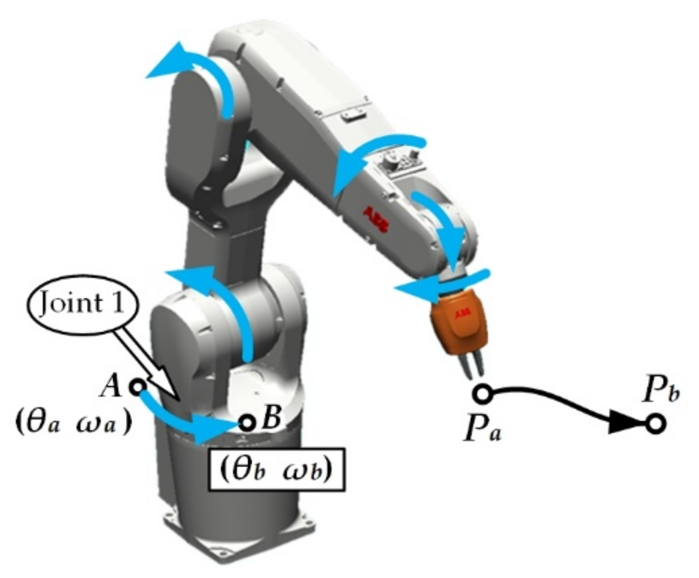
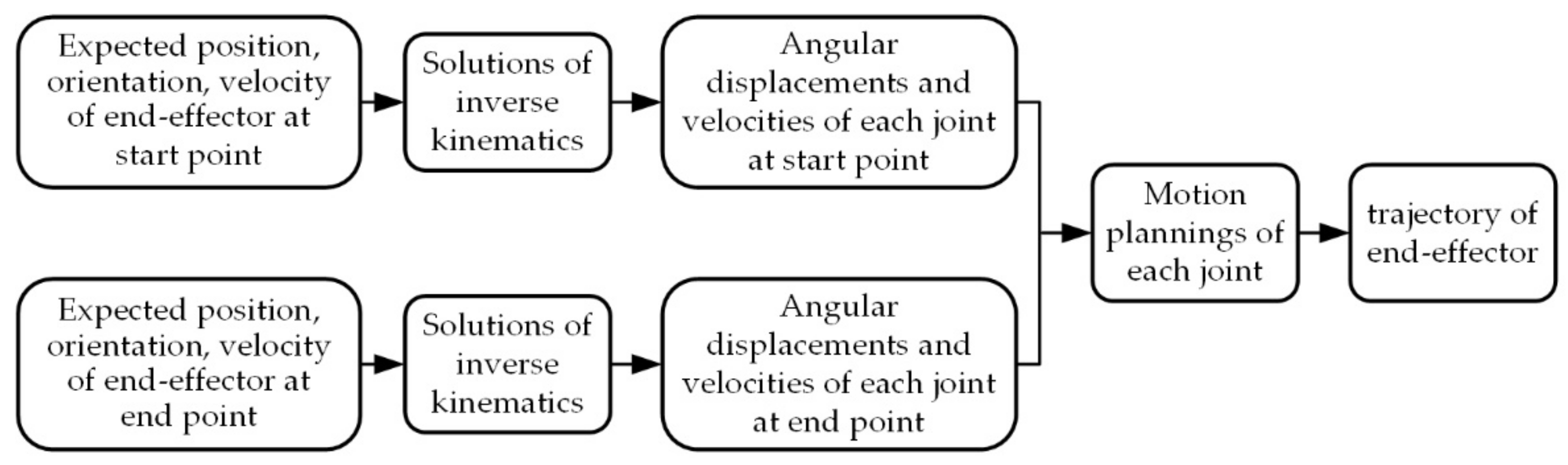
2.1. Point-to-Point Joint Motion

PTP (point to point) motion of the industrial robot is suitable for spot welding, handling, loading and unloading, circuit board insertion and other operations. In PTP motion mode, the end-effector moves from a start point to an end point. PTP motion only needs to specify positions and orientations of end-effector at the start point and end point, but the trajectory and orientations between the start point and end point are not specified or required.
When the end-effector moves in PTP mode, joints rotates normally in PTP mode as well. As shown in Figure 1, take joint 1 as an example. When the end-effector wants to move from start point Pa to end point Pb, joint 1, which is one of the six joints, needs to rotate from the start point A to end point B. In general, other joints rotate similarly. Finally, rotations of six joints work together to form the movement of the end-effector.
There is a corresponding functional relationship between the position and orientation of the end-effector and the angular displacement of each joint, as shown in formula (1). There is also a corresponding functional relationship between the end-effector velocity and the angular velocities of each joint, as shown in formula (2).
f ( θ i ) = [ x   y   z   α   β   γ ] T
J ω i T = [ v x   v y   v z   ω x   ω y   ω z ] T
In formula (1), [x y z] and [α β γ] are position and orientation of end-effector, θi are angular displacements of each joint. In formula (2), [vx vy vz] and [ωx ωy ωz] are linear velocity and angular velocity of end-effector, ωi are angular velocities of each joint, and J is the velocity Jacobian matrix. f ( θ i ) and J vary in different robots. Formulas (1) and (2) are called forward motion functions, by which the end-effector motion can be obtained from joint motion.
According to the position, orientation and speed of the end-effector, angular displacement and velocity of each joint can be obtained, which is called inverse kinematics, as shown in formulas (3) and (4) below. The speeds of the end-effector at the start and end points are zero in PTP movement so that angular velocities at the start and end points of each joint are also zero. As seen in Figure 1, the angular velocities of joint 1 at the start and end points are all equal to zero, ωa = ωb = 0.
θ i T = f 1 ( θ i ) [ x   y   z   α   β   γ ] T
ω i T = J 1 [ v x   v y   v z   ω x   ω y   ω z ] T
On the basis of angular displacement and velocity constraints at the start point and end point of each joint, motion plannings of each joint can be carried out and these joint motion plannings are finally synthesized into the end-effector motion, as shown in Figure 2.

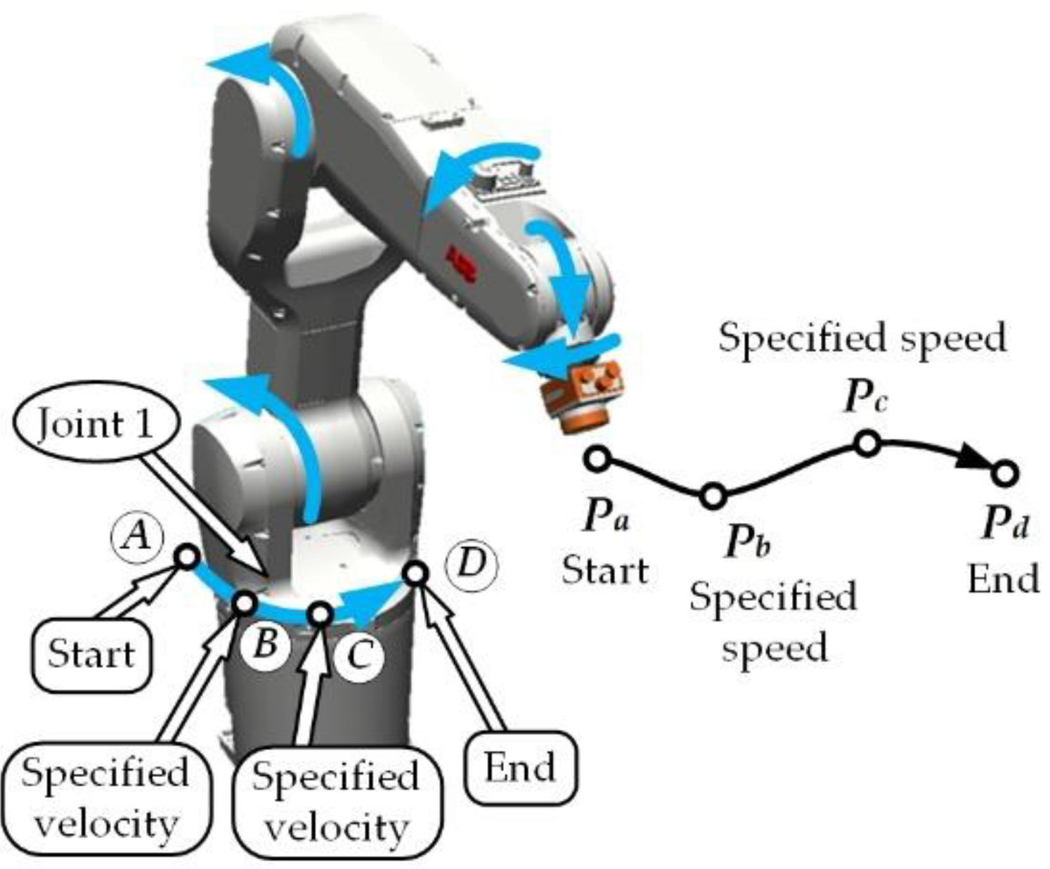
2.2. Point-to-Point Joint Motion via Multiple Points with Constrained Velocities

When there are multiple intermediate target points between the start and end points [18], and the end-effector needs to pass through these intermediate points at specified speeds, we briefly call it PTP motion with constrained speed. When the end-effector moves in speed-constrained PTP mode, joints correspondingly perform velocity-constrained PTP rotation, and both angular displacements and angular velocities at intermediate target points of joints must be specified, so as to meet position, orientation and speed requirements of the end-effector at the target points.
As shown in Figure 3, the end-effector moves from start point Pa to end point Pd. It needs to pass through two intermediate target points Pb and Pc at specified speeds, and joints should rotate accordingly. Taking joint 1 as an example, joint 1 correspondingly rotates from the start point A to end point D, passing through the intermediate target points B and C at constrained velocities. Therefore, joint 1 carries out PTP motion via multiple points at constrained velocities. By solving the inverse kinematics function, all joints’ angular displacements and angular velocities at each target point can be obtained from the positions, orientations and speeds of the end-effector, so that the rotation trajectory of joint 1 can be piecewise-planned, from point A to point B, from B to C, and from C to D. Other joints can carry out similar rotation plannings. Finally, the movement of the end-effector is synthesized by all joints’ rotations together.

3. Joint Motion Planning Method

The most used joint planning methods are cubic polynomial and quintic polynomial.

3.1. Cubic Polynomial Planning

Polynomial interpolation is commonly used to interpolate between discrete points, which is consistent with PTP motion characteristics of industrial robots, so it is often used in motion planning of industrial robots. Among the polynomials, the cubic polynomial is widely used in the PTP motion planning of industrial robots. Cubic polynomial interpolation function is shown as below formula (5):
θ ( t ) = a 0 + a 1 t + a 2 t 2 + a 3 t 3
where t is the time variable and a0, a1, a2 and a3 are four coefficients of the cubic polynomial, which need to be found out according to the boundary constraints of angular displacement and angular velocity at two adjacent target points.
Put the start time, the end time, the angular displacements and the angular velocities at the two target points into formula (5) and its first derivative, respectively. After sorting, Equation (6) for solving the coefficients can be obtained.
a 0 a 1 a 2 a 3 = 1 t 0 t 0 2 t 0 3 1 t 1 t 1 2 t 1 3 0 1 2 t 0 3 t 0 2 0 1 2 t 1 3 t 1 2 1 θ 0 θ 1 ω 0 ω 1
where, t0 is the start time, and t1 is the end time. θ0 and ω0 are respectively angular displacement and angular velocity at the first target point of a joint, and θ1 and ω1 are respectively angular displacement and angular velocity at the next target point. θ0, θ1, ω0, ω1 can be obtained through inverse kinematics. For general PTP motion, ω0 and ω1 are both zeros. For velocity-constrained PTP motion, ω0 and ω1 may not be zeros. After finding out the coefficients, the cubic polynomial planning function can be obtained, which will satisfy the boundary constraints of angular displacement and angular velocity at the target points.
Because of simplicity, clarity and small computation, the cubic polynomial is widely used in PTP joint motion planning. However, if a cubic polynomial is applied to PTP motion planning with constrained velocity, angular acceleration is discontinuous at the connecting points between every two adjacent planning segments, as shown in Figure 4c. Broken points of acceleration will cause vibrations and impacts, which is disadvantageous to the working performance and service life of the industrial robot.

3.2. Quintic Polynomial Planning

A quintic polynomial is also commonly used in the joint motion planning of industrial robots [19,20]. Quintic polynomial planning can guarantee angular acceleration continuity at the connection points between every two adjacent planning segments. A quintic polynomial function is shown in formula (7) below.
θ ( t ) = a 0 + a 1 t + a 2 t 2 + a 3 t 3 + a 4 t 4 + a 5 t 5
where t is the time variable. a0, a1, a2, a3, a4 and a5 are six coefficients of the cubic polynomial, which need to be solved according to the boundary constraints of angular displacement, angular velocity and angular acceleration at two adjacent target points.
Similarly, put the start time, the end time, the angular displacements, the velocities, and the preset accelerations at two target points into formula (7) and its first and second derivatives, respectively. After sorting, Equation (8) for solving the coefficients can be obtained.
a 0 a 1 a 2 a 3 a 4 a 5 = 1 t 0 t 0 2 t 0 3 t 0 4 t 0 5 1 t 1 t 1 2 t 1 3 t 1 4 t 1 5 0 1 2 t 0 3 t 0 2 4 t 0 3 5 t 0 4 0 1 2 t 1 3 t 1 2 4 t 1 3 5 t 1 4 0 0 2 6 t 0 12 t 0 2 20 t 0 3 0 0 2 6 t 1 12 t 1 2 20 t 1 3 1 θ 0 θ 1 ω 0 ω 1 ε 0 ε 1
where, t0, t1, θ0, θ1, ω0, ω1 have the same physical meanings as in formula (6) and εa and ε1 are the angular accelerations at the target points, which need to be given arbitrarily in advance. After finding out the coefficients, the quintic polynomial planning function can be obtained. As can be seen from Equation (8), as long as the angular accelerations at the connection point of two adjacent plannings are set equal, the angular acceleration continuity is consequent.
When a quintic polynomial is used for joint motion planning, it is required to specify in advance the angular acceleration values at target points. If the angular acceleration value is not preset appropriately, the angular velocity will fluctuate greatly. As shown in Figure 5, due to the improper preset of angular acceleration at points A and B, the angular velocity planning curve ω 1 ( t ) and curve ω 1 ( t ) between points A and B fluctuate largely. The joint motor needs to accelerate and decelerate back and forth, which is disadvantageous to the control of joint angular velocity.

4. Joint Motion Planning Based on Modified Hermite Interpolation

4.1. Function Transformation between Different Intervals

Since the variable interval of cubic Hermite interpolation is [0,1], and the variable interval of industrial robot motion planning is generally not [0,1], function transformation between different intervals is needed. There is an arbitrary function expressed as y = f ( u ) ,   u [ u 0 , u 1 ] . Given that the function is symbolically independent, this function can also be expressed as y = f ( x ) ,   x [ x 0 , x 1 ] ,   x 0 = u 0 ,   x 1 = u 1 . When the interval [x0, x1] is not equal to the interval [u0, u1], that is to say, the variable interval changes, the function expression should be transformed into the following formulas (9) and (10) in order to keep the function values of y unchanged.
u = u 0 + ( u 1 u 0 ) ( x x 0 ) ( x 1 x 0 ) , u [ u 0 , u 1 ] , x [ x 0 , x 1 ]
y = f ( u ) = f u 0 + ( u 1 u 0 ) x x 0 x 1 x 0 = f ( x ) , x [ x 0 , x 1 ]
When function interval is changed from [u0, u1] to [x0, x1], the transformed function y = f ( x ) can keep the values of the initial function y = f ( u ) unchanged, but the first-order and second-order derivatives of the function y with respect to u are no longer equal to that of the function y with respect to x, as shown in Equations (11) and (12).
d y d u = d y d x d x d u = d y d x 1 d u d x = d y d x x 1 x 0 u 1 u 0
d 2 y d u 2 = d ( d y d u )   d u = d ( d y d u )   d x d x d u = d ( d y d x x 1 x 0 u 1 u 0 )   d x 1 d u d x = d 2 y d x 2 ( x 1 x 0 u 1 u 0 ) 2
Since the variable interval of cubic Hermite interpolation is [0,1], the following Equations below can be obtained in the interval [x0,x1] instead of the interval [0,1] according to the above eqations. These formulas can be used in the following study.
u = ( x x 0 ) ( x 1 x 0 ) , u [ 0 , 1 ] , x [ x 0 , x 1 ]
y = f ( x x 0 x 1 x 0 ) , x [ x 0 , x 1 ]
d y d u = d y d x ( x 1 x 0 )
d 2 y d u 2 = d 2 y d x 2 ( x 1 x 0 ) 2

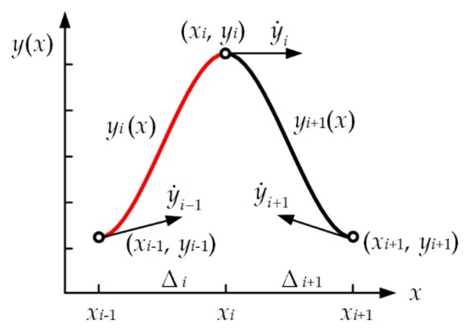
4.2. Cubic Hermite Interpolation

Cubic Hermite interpolation is a commonly used interpolation method. There is n points to be interpolated, (x0, y0), (x1, y2), …, (xn-1, yn-1). Cubic Hermite interpolation function of the i-th curve in the interval [xi-1, xi], whose interval is normalized, can be expressed as the following formula (17) in the normalized interval [21].
y i ( u ) = 1 u u 2 u 3 1 0 0 0 0 0 1 0 3 3 2 1 2 2 1 1 y i 1 y i Δ i y ˙ i 1 Δ i y ˙ i ,   u [ 0 , 1 ] ( i = 1 , 2 , , n 1 )
where n is the number of interpolated points. u is the variable derived from variable x, and the interval of u is [0,1] obtained by normalization of the interval [xi-1, xi]. yi-1 and yi are the two interpolated data points of the i-th interpolation curve. y ˙ i 1 and y ˙ i are the two first-order derivatives of y with respect to x at the points x = xi−1 and x = xi. Δi is the interval span without normalization, Δ i = x i x i 1 . According to formula (15), Δ i y ˙ i 1 and Δ i y ˙ i are the two first-order derivatives of y with respect to u at the points u = 0 and u = 1.
According to Equations (13) and (14), formula (17) can be rewritten as the following formula (18), and the variable interval is changed from [0,1] to [xi−1, xi]. The piecewise cubic Hermite interpolation curve is shown in Figure 6.
y i ( x ) = 1 x x i 1 x i x i 1 ( x x i 1 x i x i 1 ) 2 ( x x i 1 x i x i 1 ) 3 1 0 0 0 0 0 1 0 3 3 2 1 2 2 1 1 y i 1 y i ( x i x i 1 ) y ˙ i 1 ( x i x i 1 ) y ˙ i , x [ x i 1 , x i ] ( i = 1 , 2 , , n 1 )
It can be seen from formula (17) or formula (18), C0 and C1 continuity can be guaranteed as long as positions and first-order derivatives at the connection point between every two adjacent piecewise curves are specified equal. Whatever the values of y0, y1, …, yn−1 and y ˙ 0 , y ˙ 1 , …, y ˙ n 1 are assigned to, the continuity of y(x) and y ˙ ( x ) is guaranteed.
However, arbitrarily specified y ˙ 0 , y ˙ 1 , …, y ˙ n 1 cannot guarantee the continuity of the second-order derivative y ¨ ( x ) . Therefore, in order to guarantee C2 continuity of cubic Hermite curves at each knot, y ˙ 0 , y ˙ 1 , …, y ˙ n 1 must satisfy certain conditions.

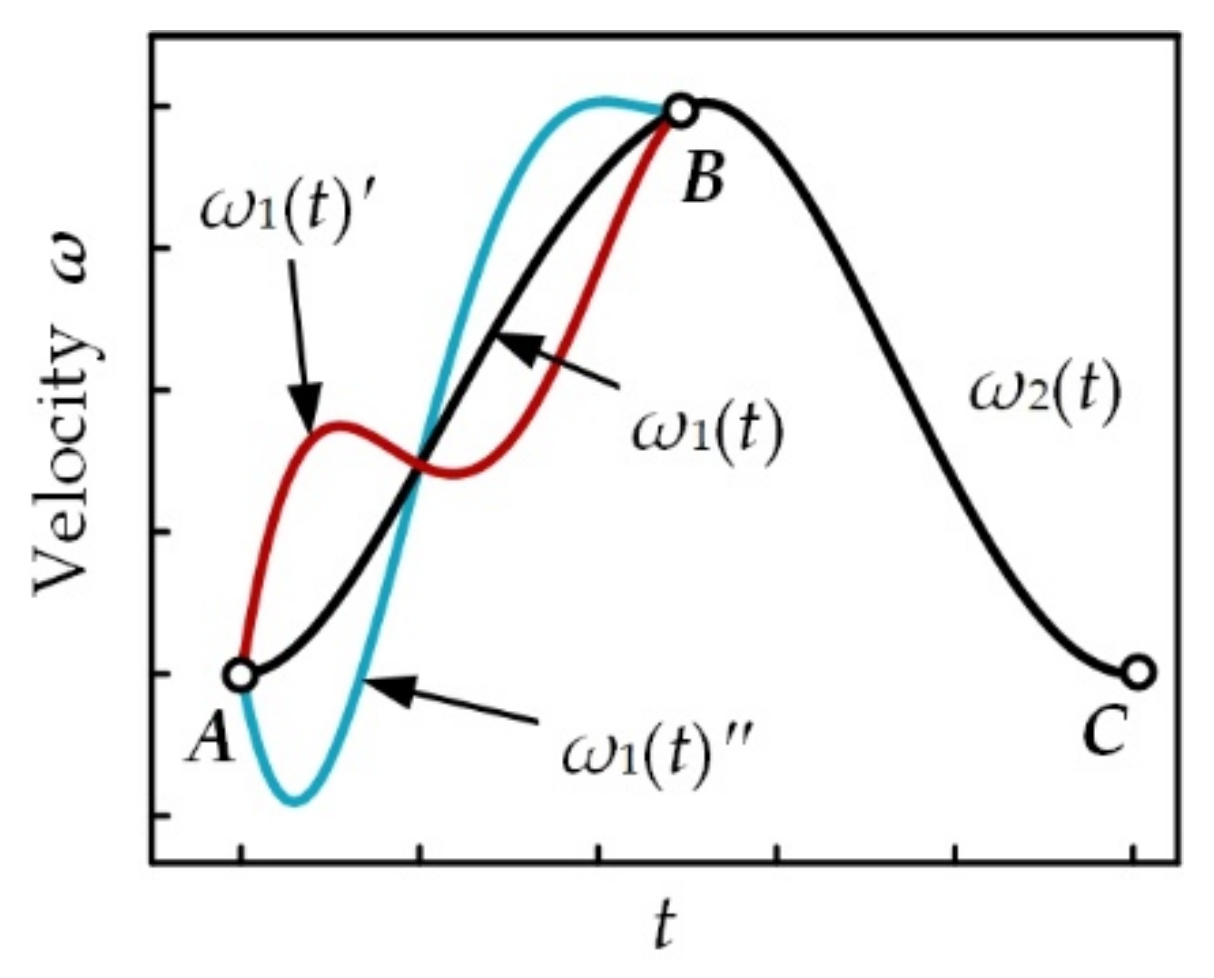
4.3. Requirement for C2 Continuity of Cubic Hermite Interpolation Curves

The requirement for C2 continuity at the connecting point between two adjacent cubic Hermite curves yi(x) and yi+1(x) is shown as the following Equation (19):
y ¨ i ( x i ) = y ¨ i + 1 ( x i )
According to Equation (18), we can obtain Equations (20) and (21) below.
y ¨ i ( x i ) = 6 ( y i 1 y i ) + 2 ( x i x i 1 ) y ˙ i 1 + 4 ( x i x i 1 ) y ˙ i ( x i x i 1 ) 2
y ¨ i + 1 ( x i ) = 6 ( y i y i + 1 ) + 4 ( x i + 1 x i ) y ˙ i + 2 ( x i + 1 x i ) y ˙ i + 1 ( x i + 1 x i ) 2
By sorting out Equations (19)–(21), formula (22) can be obtained below. First-order derivatives y ˙ i 1 , y ˙ i and y ˙ i + 1 at every three adjacent knots must meet formula (22) to guarantee C2 continuity at connection points.
( x i + 1 x i ) y ˙ i 1 + 2 ( x i + 1 x i 1 ) y ˙ i + ( x i x i 1 ) y ˙ i + 1 = 3 ( x i + 1 x i ) ( x i x i 1 ) ( y i y i 1 ) + 3 ( x i x i 1 ) ( x i + 1 x i ) ( y i + 1 y i )
formula (22) can also be rewritten as formula (23) as below.
Δ i + 1 y ˙ i 1 + 2 ( Δ i + Δ i + 1 ) y ˙ i + Δ i y ˙ i + 1 = 3 Δ i + 1 Δ i ( y i y i 1 ) + 3 Δ i Δ i + 1 ( y i + 1 y i )
It can be seen from formula (22), it is almost impossible that arbitrarily specified y ˙ 0 , y ˙ 1 , …, y ˙ n 1 at knots happen to meet formula (22). That is to say, when y ˙ 0 , y ˙ 1 , …, y ˙ n 1 at knots are constrained arbitrarily, second-order derivatives of cubic Hermite curves at connecting points are discontinuous. In fact, as for cubic Hermtime interpolation curves, only one of them can be satisfied, constraining first-order derivatives willfully at knots or C2 continuity. In order to solve the matter, a kind of modified cubic Hermite interpolation with willful constraints on first-order derivatives at knots is presented while the interpolation curves are C2 continuous.

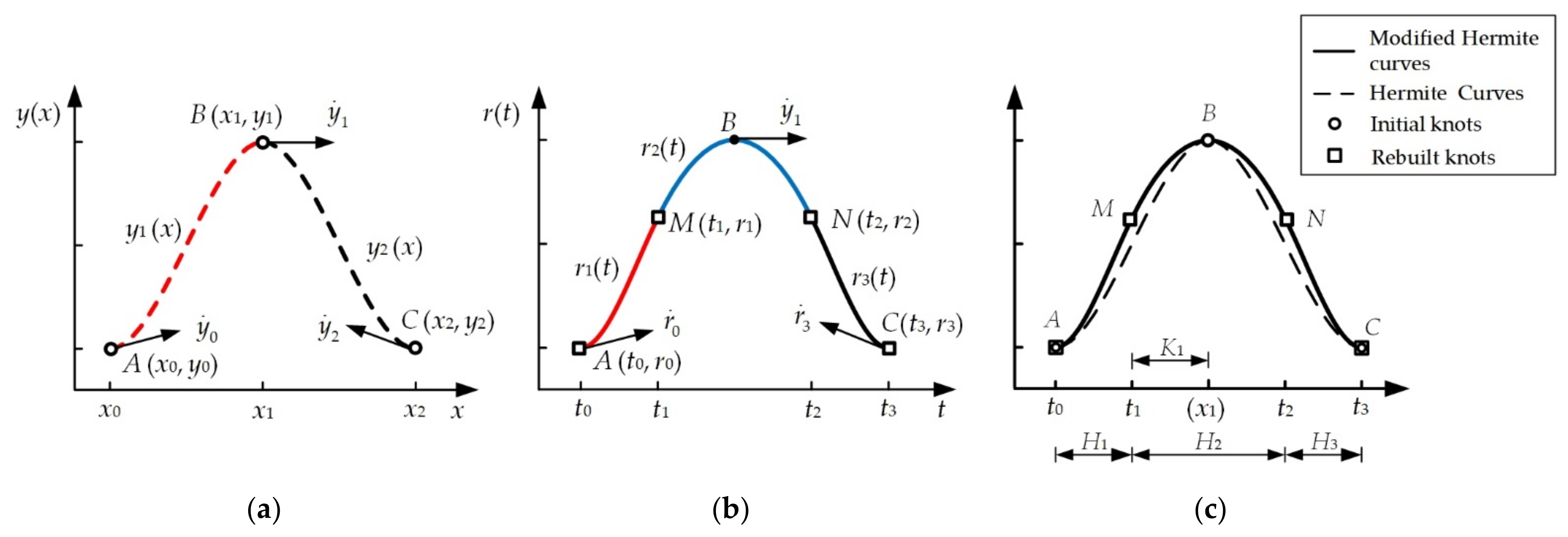
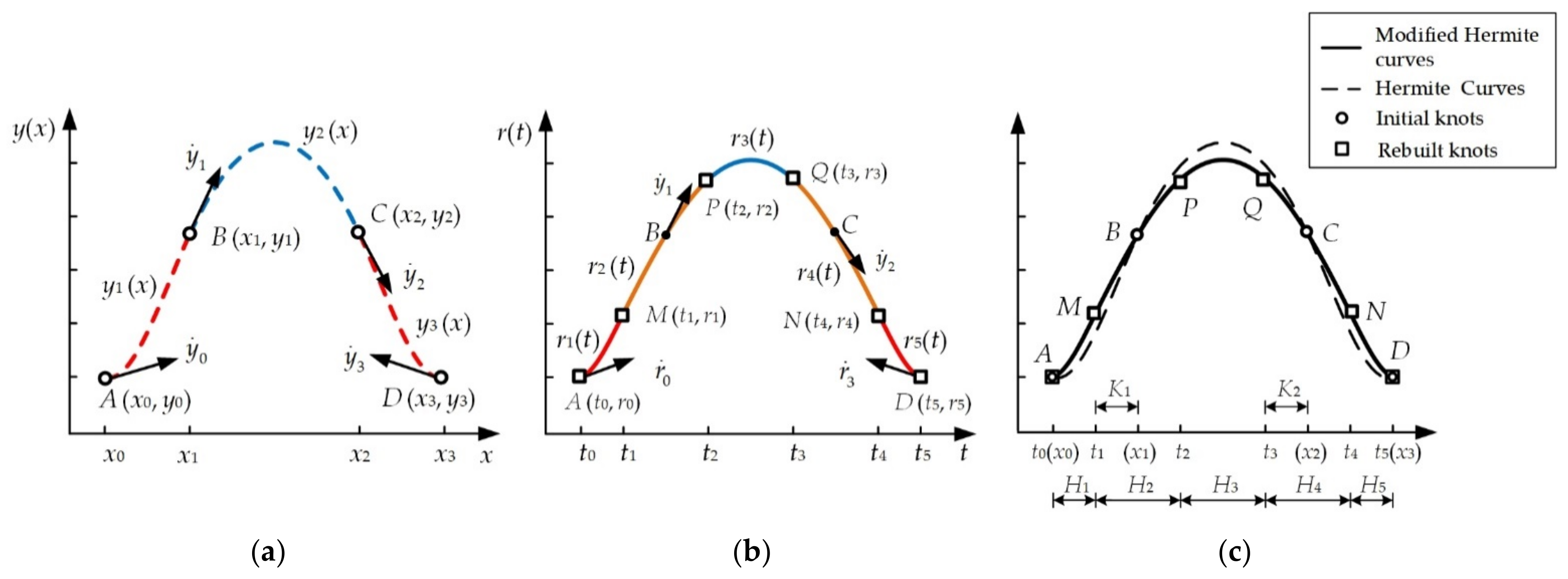
4.4. Modified Cubic Hermite Interpolation

Firstly, take three points of cubic Hermite interpolation as an example. Here are three data points to be interpolated A(x0, y0), B(x1, y1), C(x2, y2), and the first-order derivatives at knots A, B, C are assigned willfully to y ˙ 0 , y ˙ 1 and y ˙ 2 , as can be seen in Figure 7a. Since y ˙ 0 , y ˙ 1 and y ˙ 2 are specified willfully without following formula (22), the cubic Hermit interpolation curves y(x) at connection point B is not C2 continuous.
In order to specify first-order derivatives willfully at points A, B, C and guarantee C2 continuity, new points are built. As seen in Figure 7b, new point M is built between initial point A and B, and new point N is built between initial point B and C. In order to distinguish the new interpolation function from the old one, the new function is marked as r(t) instead of y(x). Newly-built knots become A(t0, r0), M(t1, r1), N(t2, r2) and C(t3, r3), and 1st derivatives at A, M, N, and C are marked respectively as r ˙ 0 , r ˙ 1 , r ˙ 2 and r ˙ 3 . The first and last point are unchanged, (x0, y0) = (t0, r0), (x2, y2) = (t3, r3), y ˙ 0 = r ˙ 0 , y ˙ 2 = r ˙ 3 .
Newly-built knots A, M, N, and C instead of initial knots A, B, and C are interpolated by cubic Hermite interpolation, and interpolating function r(t) is obtained. Function r(t) must meet the following situations: (1) Interpolating curves must pass by the knots A, B, and C; (2) First-order derivatives at point A, B, and C are equal to y ˙ 0 , y ˙ 1 and y ˙ 2 ; (3) Second-order derivatives at newly-built knots M, and N are continuous.
According to formula (18), positions and 1st derivatives at every two newly-built knots are needed to carry out interpolation. Since the first and the last point are unchanged and known, positions and 1st derivatives of new knots except point A and C must be found out. That is new points positions M(t1, r1), N(t2, r2), and their derivatives r ˙ 1 , r ˙ 2 must be found out.
Because the calculation of new knots’ ordinates t0, t1, …, tm-1 will be described in detail in a later section, t0, t1, …, tm-1 can be considered as the knowns. Therefore, firstly explain how to find out r1, r2, r ˙ 1 , r ˙ 2 .
As shown in Figure 7b, the interpolation curve r2(t) must pass by the initial knot B. According to formula (18), the second interpolation curve r2(t) can be expressed function (24) as below.
r 2 ( t ) = 1 t t 1 t 2 t 1 ( t t 1 t 2 t 1 ) 2 ( t t 1 t 2 t 1 ) 3 1 0 0 0 0 0 1 0 3 3 2 1 2 2 1 1 r 1 r 2 ( t 2 t 1 ) r ˙ 1 ( t 2 t 1 ) r ˙ 2 t [ t 1 , t 2 ]
where t is the variable, and (t1, r1), r ˙ 1 , (t2, r2) and r ˙ 2 are positions and 1st derivatives at new knot M and N, respectively.
The initial knot B(x1, y1) and its derivative y ˙ 1 must meet the interpolation function r2(t) in formula (24), which can be expressed as the following Equation (25).
r 2 ( x 1 ) = y 1 r ˙ 2 ( x 1 ) = y ˙ 1
Put x1, y1 and y ˙ 1 into formula (24). Then Equations (26) and (27) could be obtained respectively after sorting out.
1 3 K 1 2 H 2 2 K 1 3 H 2 3 K 1 2 H 2 + 2 K 1 3 H 2 K 1 2 K 1 2 K 1 3 K 1 2 K 1 3 r 1 r 2 r ˙ 1 r ˙ 2 = y 1
6 K 1 H 2 + 6 K 1 2 H 2 6 K 1 H 2 6 K 1 2 H 2 1 + 4 K 1 + 3 K 1 2 2 K 1 + 3 K 1 2 r 1 r 2 r ˙ 1 r ˙ 2 = y ˙ 1
where, x 1 t 1 is marked as K1, and t 2 t 1 is marked as H2, shown in Figure 7c. As mentioned above, the calculation of t0, t1, …, tm will be described in detail in a later section, so K1 and H2 could be considered as the knowns. Besides, y1 and y ˙ 1 are certainly the knowns of initial knot B. Therefore, Equations (26) and (27) are linear equations of the unknowns r1, r2, r ˙ 1 , r ˙ 2 . We need to solve out the unknowns r1, r2, r ˙ 1 , r ˙ 2 while there are only two Equations so that another two linear equations are required.
In order to guarantee second-order continuity at connection points, positions and first-order derivatives of new knots A, M, N and C must meet formula (22). Every three adjacent new knots among four new knots need to meet the formula (22). Specifically, knots A, M and N all together should meet formula (22). After sorting out, function (28) can be obtained.
3 H 2 H 1 3 H 1 H 2 3 H 2 H 1 3 H 1 H 2 H 2 2 ( H 1 + H 2 ) H 1 r 0 r 1 r 2 r ˙ 0 r ˙ 1 r ˙ 2 = 0
where, t 1 t 0 and t 2 t 1 are marked as H1 and H2 respectively, shown in Figure 7c. As mentioned above, H1 and H2 could be considered as the knowns. Since r0 and r ˙ 0 are the ordinate and 1st derivative of knot A, they are known constants. Hence, Equation (28) is a linear one of the unknowns r1, r2, r ˙ 1 and r ˙ 2 .
Moreover, new knots M, N and C all together should also meet the formula (22). Similarly, Equation (29) can be obtained after sorting out.
3 H 3 H 2 3 H 2 H 3 3 H 3 H 2 3 H 2 H 3 H 3 2 ( H 2 + H 3 ) H 2 r 1 r 2 r 3 r ˙ 1 r ˙ 2 r ˙ 3 = 0
where, t 2 t 1 and t 3 t 2 are marked as H2 and H3. H2 and H3 could be considered as known constants. Since r3 and r ˙ 3 are the ordinate and 1st derivative of knot C, they are the knowns. Hence, Equation (29) is also a linear one of the unknowns r1, r2, r ˙ 1 and r ˙ 2 .
These four Equations (26)–(29) are all linear ones of the unknowns r1, r2, r ˙ 1 and r ˙ 2 . By solving the Equations, the values of r1, r2, r ˙ 1 and r ˙ 2 can be obtained. After acquiring the positions and the 1st derivatives at newly-built knots A, M, N, and C, modified cubic Hermite interpolation curves can be obtained according to formula (18).
Now let us look at the situation with four initial points interpolated. As seen in Figure 8a, there are four initial knots to be interpolated A(x0, y0), B(x1, y1), C(x2, y2), and D(x3, y3). The first-order derivatives at knots A, B, C and D are assigned willfully to y ˙ 0 , y ˙ 1 , y ˙ 2 , and y ˙ 3 . Rebuild new data points. As seen in Figure 8b, new knot M is built between the first and the second knots A and B, and new knot N between the penultimate and the last knot C and D. It must be noted that two new knots P and Q need to be built between knot B and C. If only one new knot is built between knots B and C, set of Equations cannot be solved because the number of Equations is greater than that of the unknowns. Similarly, we need to find out the unknowns r1, r2, r3, r4, r ˙ 1 , r ˙ 2 , r ˙ 3 , r ˙ 4 of the newly-built knots except the first and the last one.
In the same way, the initial knot B(x1, y1) and its derivative y ˙ 1 must meet the interpolation function r2(t). The initial knot C(x2, y2) and its derivative y ˙ 2 must meet the interpolation function r4(t), shown in Figure 8b. Then put x1, y1, y ˙ 1 and x2, y2, y ˙ 2 into r2(t) and r4(t) derived from formula (18), and we can get four Equations similar to Equations (26) and (27). When it is extended to more knots, Equations (30) and (31) can be obtained after sorting and inducting.
1 3 K i 2 H j + 1 2 K i 3 H j + 1 3 K i 2 H j + 1 + 2 K i 3 H j + 1 K i 2 K i 2 K i 3 K i 2 K i 3 r j r j + 1 r ˙ j r ˙ j + 1 = y i ( i = 1 , 2 , 3 , , n 2 ) ( j = 1 , 3 , 5 , , m 3 )
6 K i H j + 1 + 6 K i 2 H j + 1 6 K i H j + 1 6 K i 2 H j + 1 1 + 4 K i + 3 K i 2 2 K i + 3 K i 2 r j r j + 1 r ˙ j r ˙ j + 1 = y ˙ i ( i = 1 , 2 , 3 , , n 2 ) ( j = 1 , 3 , 5 , , m 3 )
where, n is the number of the initial knots ( n 3 ), and m ( m = 2 n 2 ) is the number of the newly-built knots. The subscript i is related to initial knots while subscript j is related to newly-built knots. Array y is the ordinates of initial knots, y0, y1, …, yn-1, which are all knowns. The array y ˙ is the first-order derivatives of initial knots, y ˙ 0 , y ˙ 1 , …, y ˙ n 1 , which are all knowns. Array r is the ordinates of newly-built knots, r0, r1, …, rm-1, in which r0 and rm-1 are knowns and others are unknowns. The array r ˙ is the first-order derivatives of newly-built knots r ˙ 0 , r ˙ 1 , …, r ˙ m 1 , in which r ˙ 0 and r ˙ m 1 are knowns and others are unknowns. So, r1, r2, … , rm-2 and r ˙ 1 , r ˙ 2 , …, r ˙ m 2 are unknown.
The expressions of array K and array H are shown in Equations (32) and (33) below respectively, seen as in Figure 8c for graphic representation. Since all of the initial knots’ abscissas x0, x1, … , xn-1 are given and the newly-built knots’ abscissas t0, t1, … , tm-1 can be considered as the knowns described in the latter section, array K and array H are known constants. Hence, Equations (30) and (31) are linear ones.
K i = x i t j ( i = 1 , 2 , 3 , , n 2 , j = 1 , 3 , 5 , , m 3 )
H j = t j t j 1   (   j = 1 , 2 , , m 1 )
Synthesizing formulas (30) and (31), there are 4 ( n 2 ) unknowns and 2 ( n 2 ) Equations. Hence, the set of Equations has no unique solution unless other Equations are to be added.
Similarly, in order to guarantee C2 continuity at newly-built knots, the positions and first-order derivatives of new knots A, M, N, P, Q and D in Figure 8b must meet the formula (22). Every three adjacent new knots need to meet the formula (22). When it is extended to more knots, Equation (34) can be obtained after sorting and inducting.
3 H j + 1 H j 3 H j H j + 1 3 H j + 1 H j 3 H j H j + 1 H j + 1 2 ( H j + H j + 1 ) H j r j 1 r j r j + 1 r ˙ j 1 r ˙ j r ˙ j + 1 = 0 ( j = 1 , 2 , 3 , , m 2 )
where, the meanings of m ( m = 2 n 2 ) , r, r ˙ and H are the same as that of the above. Equation (34) are linear ones. It is pointed out that r0, r m 1 , r ˙ 0 , r ˙ m 1 of the first and last new point are knowns. The unknowns are r1, r2, … , rm-2 and r ˙ 1 , r ˙ 2 , …, r ˙ m 2 . Here are 4 ( n 2 ) the unknowns and 2 ( n 2 ) Equations. Combining with formulas (30), (31) and (34), the number of the unknowns is 4 ( n 2 ) , and the number of the Equations is 4 ( n 2 ) . Therefore, set of Equations (30), (31) and (34) are all linear Equations and have a unique solution.
After positions and first-order derivatives of newly-built knots are found out, modified piecewise cubic Hermite curves can be obtained according to formula (18). The modified curves would pass by the initial knots, and first-order derivatives at the initial knots can be specified at will while the curves are C2 continuous.
For more than four initial points to be interpolated, every two new points need to be built between every two initial points from the second and penultimate initial point. The method is similar to the one for four initial points.

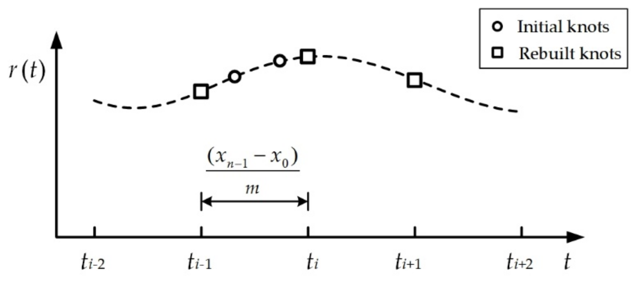
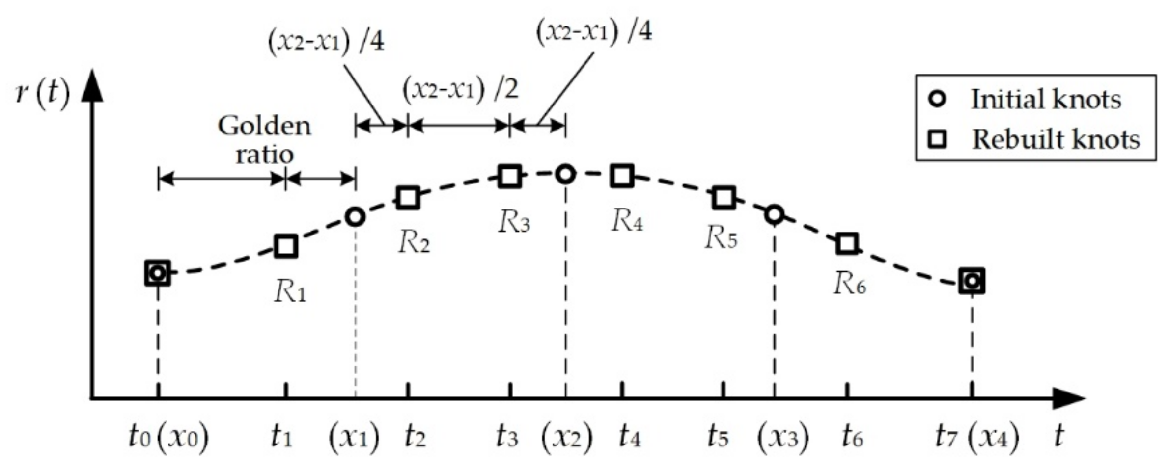
4.5. Arrangement for The Abscissas of Newly-Built Knots

Given n initial knots to be interpolated denoted as (xi−1, yi−1), I = 1, 2, …, n, ( n 3 ). The abscissas of initial knots are x0, x1, … , xn−1. New knots are built for proposed interpolation, marked as (rj−1, tj−1), j = 1, 2, …, m, ( m = 2 n 2 ). The abscissas of new knots are t0, t1, … , tm−1. We need to arrange t0, t1, … , tm−1 according to x0, x1, … , xn−1.
The first idea is to average t0, t1, … , tm−1. Uniform abscissa knots are beneficial to the smoothness of the interpolation curves. However, averaging t0, t1, … , tm−1 may possibly lead to the situation that there are two initial knots existing between two new knots, seen in Figure 9. Since a piecewise curve must pass by the two initial points, too many constraints are imposed on this curve so that the curve function cannot be solved and interpolation functions cannot be found out.
To avoid the trouble mentioned above, the following scheme is proposed on the basis of homogenization as much as possible. Take five initial knots for example. As can be seen in Figure 10, two newly-built knots R2 and R3 are built between the second and the third initial as described above.
Based on the principle of average for new knots, the horizontal distance between the second and the third initial points is divided into three segments, so the abscissas t2 and t3 of the new knots R2 and R3 can be expressed as Equations (35) and (36) below. The same scheme is applied whenever there are two newly-built knots between every two adjacent initial points.
t 2 = x 1 + 1 4 ( x 2 x 1 )
t 3 = x 1 + 3 4 ( x 2 x 1 )
Between the first and the second initial points, is there only one newly-built knot R1 inserted, seen in Figure 10. The horizontal distance between the first and the second initial knots is divided by new point R1 into two segments with unequal length, so the golden ratio is a reasonable method. Consequently, the abscissa t1 of newly-built knot R1 can be expressed by Equation (37). The same is as for the last newly-built knot R6, and the abscissa t6 of the newly-built knot R6 can be expressed by Equation (38).
t 1 = x 0 + 0.618 ( x 1 x 0 )
t 6 = x 4 0.618 ( x 4 x 3 )
Extended to the case that the number of the initial points is n ( n 4 ), formula (39) can be obtained. Abscissas of all newly-built knots t are acquired from the abscissas of initial knots x. If there are only three initial points ( n = 3 ), take the first two Equations and the last two Equations in formula (39).
t 0 = x 0 t 1 = x 0 + 0.618 ( x 1 x 0 ) t j = x i 1 + 1 4 ( x i x i 1 ) i = 2 , 3 , , n 2 , j = 2 , 4 , 6 , , m 4 t j + 1 = x i 1 + 3 4 ( x i x i 1 ) t m 2 = x n 1 0.618 ( x n 1 x n 2 ) t m 1 = x n 1
where n and m ( m = 2 n 2 ) are respectively the numbers of initial and newly-built knots. The subscript i is related to the initial knots while subscript j is related to the newly-built knots.

4.6. Summary

Sum up the steps of modified cubic Hermit interpolation as follows:
(1)
According to the abscissas of given initial knots x0, x1, … , xn−1, ( n 3 ), the abscissas of newly-built knots, t0, t1, … , tm−1, ( m = 2 n 2 ), are arranged and calculated by the formula (39).
(2)
According to the given positions and the 1st derivatives of the initial points and the abscissas of the newly-built knots achieved in step 1, a set of linear equations are obtained by formulas (30)–(34). Then, the ordinates and the first derivatives of the newly-built knots are acquired via solving the set of linear equations.
(3)
According to the positions and first-order derivatives of newly-built knots achieved in previous steps, modified cubic Hermite interpolation curves are obtained by formula (18).

5. Case Study

In order to verify the rationality and effectiveness of the proposed methodology, the following study case is employed. The usage of the proposed methodology is further described in detail during the study case analysis.
Case: In order to accomplish a task, joint 1 of the industrial robot needs to carry out velocity-constrained PTP motion. As shown in Figure 11a, joint 1 turns from start target point A to intermediate target points B, C and to end target point D in turn. The velocities at the intermediate target points B and C are specified. The rotational requirements at each target point are shown in Table 1. Using the proposed planning of modified cubic Hermite interpolation presented above, carry out velocity-constrained PTP motion planning for joint 1.
There are four initial knots A, B, C, and D to be interpolated. As seen in Figure 11b, newly-built knot M needs to be inserted between initial A and initial B, and N between C and D, and P, Q between B and D, according to the proposed method. Therefore, the initial knots A, B, C, D are replaced by the newly-built knots A, M, P, Q, N, and D. The initial time knots become the newly-built time knots correspondingly. In order to be unified with the previous formula, the initial time knot is denoted as x, and the newly-built time knots is denoted as t. According to formula (39), the newly-built time knots are arranged from the initial time knots x = 0, 5, 15, 25 (s) and the newly-built time knots are t = 0, 3, 8, 13, 19, 25 (s) respectively with proper rounding.
We need to find out the angular displacements and angular velocities at the newly-built knots M, P, Q and N from the initial knots A, B, C, and D. According to formula (30), 31, 32, 33, and 34, we can obtain Equation (40) to solve out the angular displacements and angular velocities of the rebuilt knots, θM, θP, θQ, θN, ωM, ωP, ωQ, ωN.
0.4 0.225 0 0 2 0.375 0 0 0.3 0 0.3 0 0.5 2 0.5 0 0 0.327 0.1 0.227 0 0.546 2 0.455 0 0 0.25 0 0 0 0.5 2 0.648 0.352 0 0 0.72 0.48 0 0 0.288 0.288 0 0 0.12 0.32 0 0 0 0 0.741 0.259 0 0 0.889 0.444 0 0 0.222 0.222 0 0 0 0.333 θ M θ P θ Q θ N ω M ω P ω Q ω N = 0 0 0 45 30 8 90 8
The values of θM, θP, θQ, θN, ωM, ωP, ωQ, ωN can be obtained by solving the linear Equations. In addition to the previously calculated amount of time, the information of the newly-built knots for joint motion planning can be listed in Table 2.
According to the motion conditions at newly-built target points in Table 2, the piecewise motion planning of joint 1 can be carried out by formula (18).
The planning function of AM segment is shown in Equation (41) below.
θ 1 ( t ) = 2.221 t 2 0.214 t 3 0 t 3
The planning function of the MP segment is shown in Equation (42) below.
θ 2 ( t ) = 4.142 + 4.142 t + 0.84 t 2 0.061 t 3 3 t 8
The planning function of the PQ segment is shown in Equation (43) below.
θ 3 ( t ) = 76.069 + 31.115 t 2.531 t 2 + 0.08 t 3 8 t 13
The planning function of the QN segment is shown in Equation (44) below.
θ 4 ( t ) = 125.677 15.442 t + 1.05 t 2 0.012 t 3 13 t 19
The planning function of the ND segment is shown in Equation (45) below.
θ 5 ( t ) = 1057.847 162.627 t + 8.796 t 2 0.148 t 3 19 t 25
Validate whether the motion planning functions meet the requirements of angular displacements and angular velocities at the initial target points, as shown in Table 3. Validation results show the planning functions meet the requirements.
Validate the continuities of the motion planning functions at the connecting points between every two adjacent planning segments, as shown in Table 4. The validation results show that angular displacements, angular velocities and angular accelerations at connecting points are all continuous.
According to the motion planning functions above, the motion planning curves can be obtained, shown in Figure 12. As can be seen from Figure 12a, the angular displacement curve is very smooth and meets the angular displacement requirements at the initial target points A, B, C, D. As can be seen from Figure 12b, the angular velocity curves are also smooth, the velocity fluctuation is gentle, and meets the angular velocity requirements at the initial target points A, B, C, D. As can be seen from Figure 12c, the angular acceleration curves are continuous at the connecting points M, P, Q, N, and the whole acceleration curves does not fluctuate much.
The motion planning curves once more verify that the motion planning functions can not only meet the constrained requirements of angular displacements and angular velocities at the initial target points but also guarantee the continuity of angular acceleration and angular velocity fluctuates gently. It proves that the proposed method can be applied well to joint motion planning with velocity constraints, and avoid the problems of discontinuous angular acceleration in cubic polynomial planning and large fluctuation of angular velocity in the quintic polynomial.

6. Comparison and Discussion

In order to compare with the proposed planning methodology, the most commonly used PTP joint planning method, cubic polynomial and quintic polynomial, are applied to the same case study above as well. The results of the study and analysis below reflect there are more or fewer deficiencies for these two methods to be used for joint planning with constrained velocity. The detailed comparison and analysis process are as follows.
Figure 13 shows the angular displacement curves obtained by the proposed methodology, cubic polynomial, and quintic polynomial respectively. As can be seen from Figure 13a,b, the angular displacement curve obtained by the proposed method is similar to the curves obtained by the cubic polynomial. Both of the curves are smooth and the fluctuation is very small. In Figure 13c, the angular displacement curves obtained by quintic polynomial fluctuate a little bit. In fact, a curve with a higher order is more likely to fluctuate than a curve with a lower order. Therefore, we should try to avoid using higher-order functions for planning.
Figure 14 is the angular velocity curves obtained by these three methods. In Figure 14a, the velocity curves obtained by the proposed method are smooth, the velocity fluctuation is gentle, and the variation trend is roughly similar to that in Figure 14b by the cubic polynomial. In Figure 14b, the overall velocity waveform by a cubic polynomial is simple and appropriate. However, there are turning points at junctions B and C, which will lead to discontinuous angular acceleration at the connection points. In Figure 14c, the overall fluctuation of the velocity curves by a quintic polynomial is obviously large. In particular, because of inappropriate preset angular acceleration at point C, the velocity near point C fluctuates back and forth sharply, which is not conducive to the control of joint rotation speed. This shows that quintic polynomial planning is likely to cause angular velocity to fluctuate too much. Moreover, the higher the order of the polynomial is, the higher the velocity peak will be, which makes greater volatility. These are the weaknesses of quintic polynomial planning.
Figure 15 is the angular acceleration curves obtained by these three methods. As can be seen from Figure 15a,c, the angular acceleration curves, obtained by proposed methodology and quintic polynomial respectively, are both continuous at connection points. Because the order of the quintic polynomial is high, the angular acceleration in Figure 15c is also easy to fluctuate. In Figure 15b, the angular acceleration curves obtained by cubic polynomial are obviously broken at the connecting points B and C. The angular acceleration discontinuity of the joint will cause vibrations and impacts, which will degrade the working performance and decrease the service life of industrial robots.
It can be seen from the above comparative analysis of this case, as for joint PTP motion planning with constrained velocity, the angular acceleration of cubic polynomial planning is discontinuous, which will lead to vibrations and impacts. Angular velocity of quintic polynomial planning fluctuates greatly back and forth, which is not conducive to velocity control. The proposed motion planning methodology not only meets the constraints of angular displacements and angular velocities at target points but also guarantees the continuity of angular acceleration. The maximum function order of proposed planning is three, which effectively avoids the fluctuation caused by high-order functions.

7. Conclusions

For the industrial robots’ PTP joint motion planning with velocity constraint, cubic polynomial planning has the problem of angular acceleration discontinuity, which will cause vibrations and impacts. As for quintic polynomial planning, angular accelerations at target points need to be given in advance and because it is hard to give appropriate angular accelerations in advance, it will lead to large velocity fluctuations which are not conducive to velocity control.
In order to solve these problems in joint planning, a kind of methodology based on modified Hermite interpolation is proposed. On the basis of Hermite interpolation, new target knots are reconstructed from the initial target knots. Then, newly-built knots instead of old initial knots are used to carry out joint motion planning. Using the proposed methodology, not only does the motion planning meet the requirements for angular displacement and angular velocity at the initial knots, but also the angular acceleration of the whole planning is continuous without broken points. Moreover, the maximum order of the planning functions is three, which avoids the velocity fluctuation caused by the higher-order functions such as quintic polynomial. Therefore, the problems existing in cubic polynomial planning and quintic polynomial planning can be solved well.
A study case is given to verify the rationality and effectiveness of the proposed method. The case study results show that, compared with the other two planning methods, the proposed methodology is applied well to PTP joint motion planning with velocity constraints, and is conducive to the working performance and service life of industrial robots.
In the future, efforts will be made on optimization investigation as continued research in the area. The basic motion planning of industrial robots, including improved motion planning, focuses on the continuity and smoothness of the trajectory. However, efficiency, energy, impact and other problems in the actual operation requirements are not considered. Thus, optimization of single or multiple objectives among efficiency, energy, the impact will be the further potential studies on the basis of the motion planning. Moreover, motion planning needs to be realized through motion control. Due to strong nonlinear coupling between each joint and end-effector, there will be disturbances, errors and other uncertain factors, so optimal control will also be considered as a further investigation to guarantee motion planning realized precisely.

Author Contributions

Conceptualization, Y.S.; Investigation, X.L. and P.Z.; Funding acquisition, Y.S. and P.Z.; Writing—original draft, Y.P.; Validation, W.Z. and Y.P.; Methodology, Y.P. and W.Z.; Writing—review and editing, Y.P., Y.S. and X.L. All authors have read and agreed to the published version of the manuscript.

Funding

This research was funded by the “National Science and Technology Major Project of China, grant number 2017-VII-0002-0095” and the “Aeronautical Science Foundation of China, grant number 2020Z045053001”.

Institutional Review Board Statement

Not applicable.

Informed Consent Statement

Not applicable.

Data Availability Statement

Not applicable.

Conflicts of Interest

The authors declare no conflict of interest.

References

  1. Uhlmann, E.; Heitmüller, F. Improving Efficiency in Robot Assisted Belt Grinding of High Performance Materials. Adv. Mater. Res. 2014, 907, 139–149. [Google Scholar] [CrossRef]
  2. Kraljić, D.; Kamnik, R. Trajectory Planning for Additive Manufacturing with a 6-DOF Industrial Robot. Mech. Mach. Sci. 2018, 456–465. [Google Scholar]
  3. Biagiotti, L.; Melchiorri, C. Trajectory Planning for Automatic Machines and Robots; Springer: Berlin, Germany, 2008; pp. 1–3. [Google Scholar]
  4. Chettibi, T. Smooth point-to-point trajectory planning for robot manipulators by using radial basis functions. Robotica 2019, 37, 539–559. [Google Scholar] [CrossRef]
  5. Li, L.; Shang, J.Y.; Feng, Y.L. Research of trajectory planning for articulated industrial robot: A review. Comput. Eng. Appl. 2018, 54, 36–50. [Google Scholar]
  6. Gasparetto, A.; Zanotto, V. A new method for smooth trajectory planning of robot manip-ulators. Mech. Mach. Theory 2007, 42, 455–471. [Google Scholar] [CrossRef]
  7. Xu, J.; Mei, J.; Duan, X. An algorithm for segment transition in continuous trajectory planning of industrial robot. Chin. J. Eng. Des. 2016, 23, 537–543. [Google Scholar]
  8. Choi, Y.; Kim, D.; Hwang, S.; Kim, H.; Kim, N.; Han, C. Dualarm robot motion planning for collision avoidance using B-spline curve. Int. J. Precis. Eng. Manuf. 2017, 18, 835–843. [Google Scholar] [CrossRef]
  9. Meike, D.; Ribickis, L. Industrial robot path optimization approach with asynchronous fly-by in joint space. In Proceedings of the 2011 IEEE International Symposium on Industrial Electronics, Gdansk, Poland, 27–30 June 2011. [Google Scholar]
  10. Dyllong, E.; Komainda, A. Local Path Modifications of Heavy Load Manipulators. In Proceedings of the IEEE/ASME International Conference on Advanced Intelligent Mechatronics, Como, Italy, 8–12 July 2001; pp. 464–469. [Google Scholar]
  11. Abbas, A.; Nasri, A.; Maekawa, T. Generating B-spline curves with points, normals and curvature constraints: A constructive approach. Vis. Comput. 2010, 26, 823–829. [Google Scholar] [CrossRef]
  12. Gofuku, S.; Tamura, S.; Maekawa, T. Point-Tangent/Point-Normal B-Spline Curve Interpolation by Geometric Algorithms. Comput. Aided Des. 2009, 41, 412–422. [Google Scholar] [CrossRef]
  13. Xu, X.; Wang, X.; Qin, F. Trajectory planning of robot manipulators by using spline function approach. In Proceedings of the World Congress on Intelligent Control and Automation IEEE, Hefei, China, 28 June–2 July 2000. [Google Scholar]
  14. Niku, S.B. Introduction to Robotics: Analysis, Control, Applications, 3rd ed.; Wiley-Blackwell: Hoboken, NJ, USA, 2020; pp. 260–263. [Google Scholar]
  15. Parikh, P.; Trivedi, R.; Dave, J. Trajectory Planning for the Five Degree of Freedom Feeding Robot Using Septic and Nonic Function. Int. J. Mech. Eng. Robot. Res. 2020, 9, 1043–1050. [Google Scholar] [CrossRef]
  16. Boryga, M.; Graboś, A. Planning of manipulator motion trajectory with higher-degree polynomials use. Mech. Mach. Theory 2009, 44, 1400–1419. [Google Scholar] [CrossRef]
  17. Perez Bailon, W.; Barrera Cardiel, E.; Juarez Campos, I.; Ramos Paz, A. Mechanical energy optimization in trajectory planning for six DOF robot manipulators based on eighth-degree polynomial functions and a genetic algorithm. In Proceedings of the IEEE 7th International Conference on Electrical Engineering, Computing Science and Automatic Control, Tuxtla Gutierrez, Mexico, 8–10 September 2010. [Google Scholar]
  18. Zacharia, P.T.; Xidias, E.K.; Aspragathos, N.A. Task scheduling and motion planning for an industrial manipulator. Robot. Comput. Integr. Manuf. 2013, 29, 449–462. [Google Scholar] [CrossRef]
  19. Perumalsamy, G.; Visweswaran, P.; Jose, J. Quintic interpolation joint trajectory for the path planning of a serial two-axis robotic arm for PFBR steam generator inspection. In Machines, Mechanism and Robotics; Springer: Singapore, 2018; pp. 637–648. [Google Scholar]
  20. Liu, S.; Du, H.; Wang, S.; Zhao, Y. Path Planning and System Simulation for an Industrial Spot Welding Robot Based on SimMechanics. Key Eng. Mater. 2009, 419, 665–668. [Google Scholar] [CrossRef]
  21. Chang, Z.; Wan, Y. Computer Aided Geometric Design Technology, 3rd ed.; Science Press: Beijing, China, 2013; p. 26. [Google Scholar]
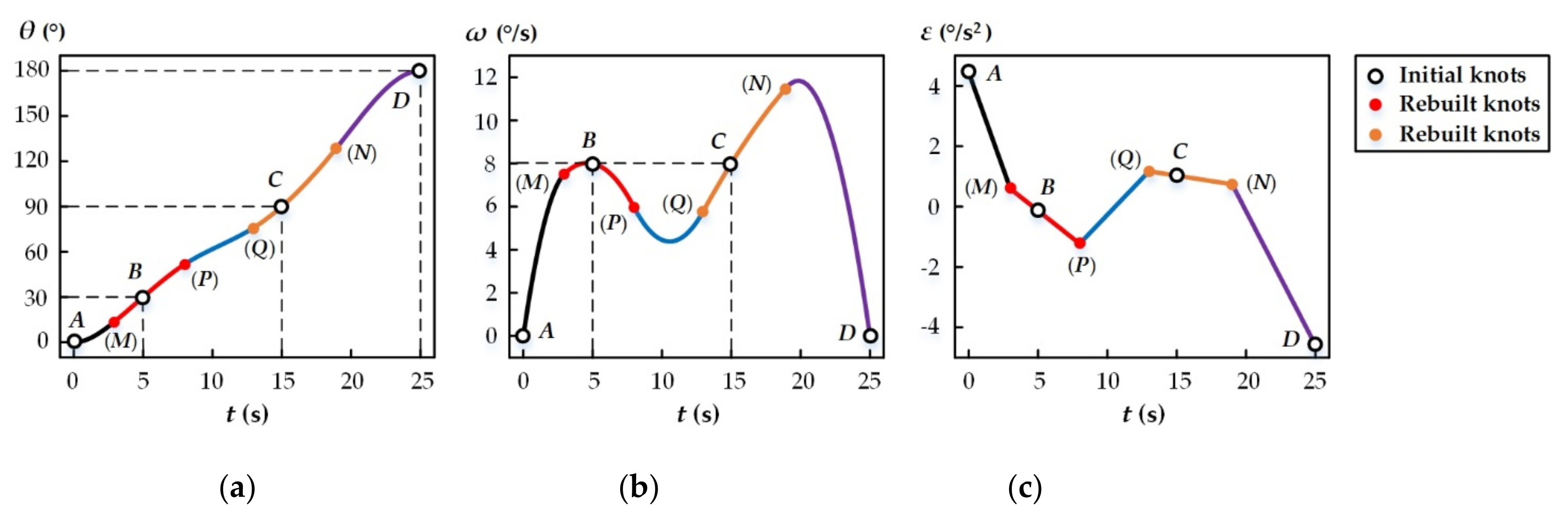
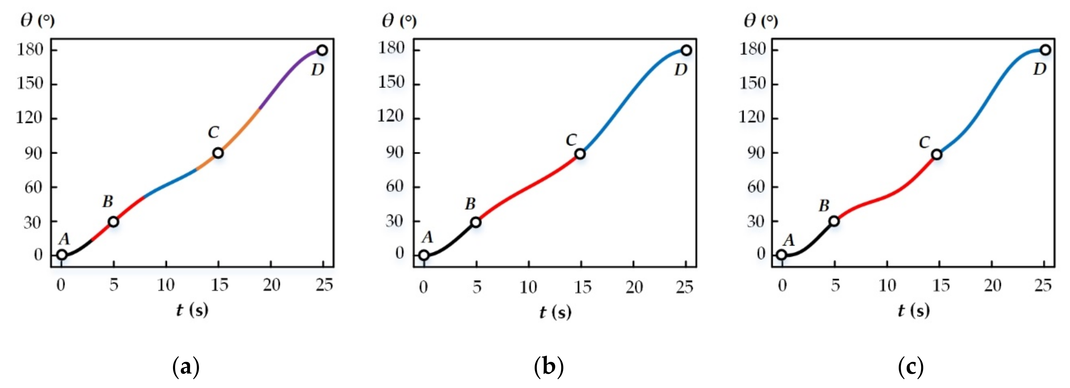
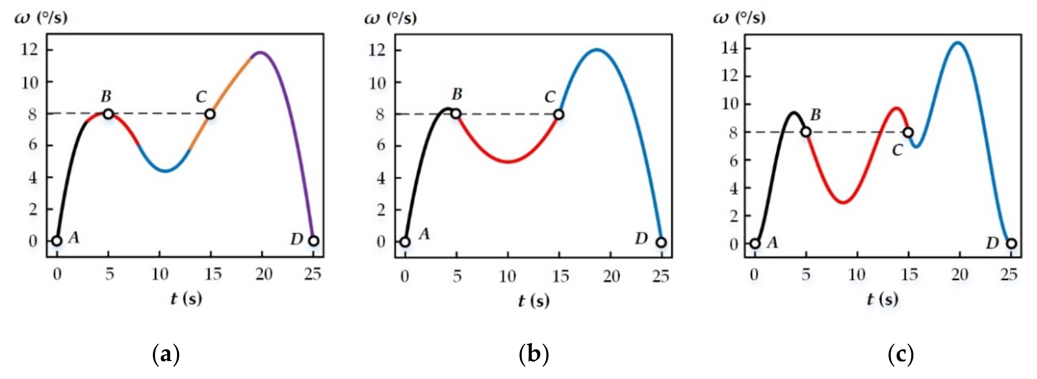
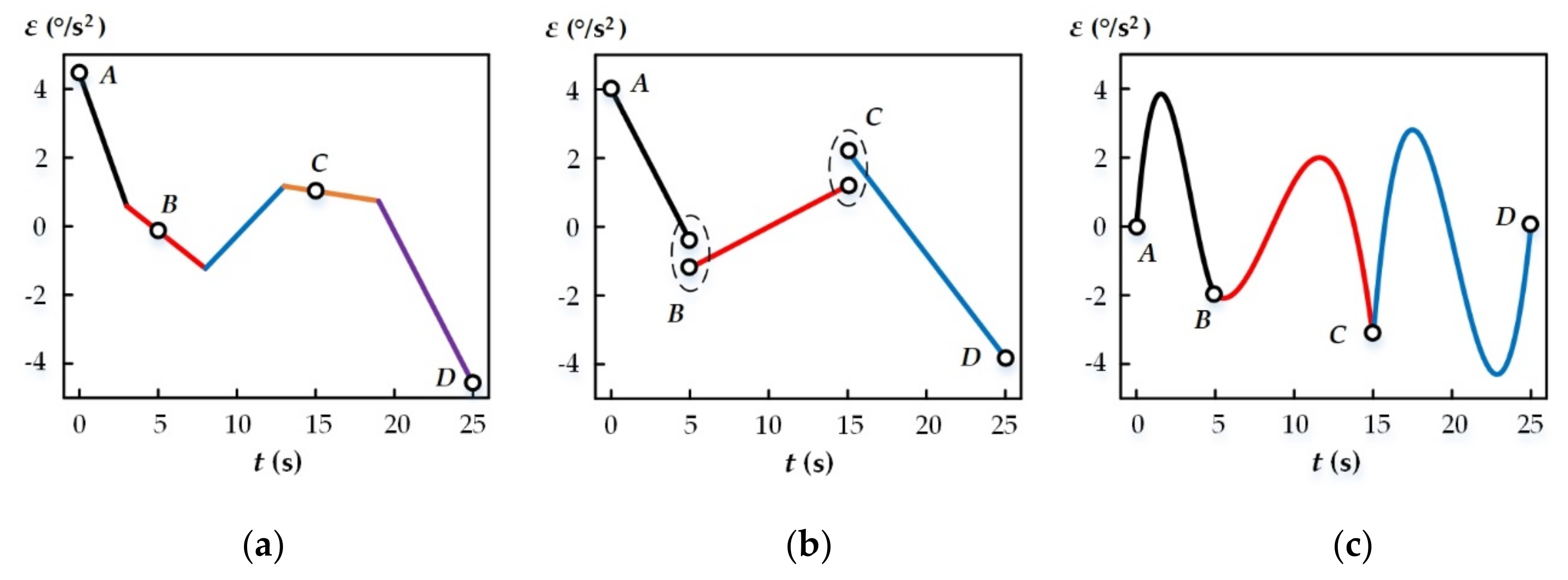
Figure 1. Point-to-Point movement.
Applsci 11 08879 g001
Figure 2. Relationship between PTP end-effector motion and PTP motion plannings of joints.
Applsci 11 08879 g002
Figure 3. PTP motion with constrained velocities.
Applsci 11 08879 g003
Figure 4. Velocity-constrained PTP motion planning by cubic polynomial interpolation: (a) Angular displacement planning; (b) Angular velocity planning; (c) Angular acceleration planning.
Applsci 11 08879 g004
Figure 5. Angular velocity fluctuation in quintic polynomial planning.
Applsci 11 08879 g005
Figure 6. Piecewise cubic Hermite interpolation curves.
Applsci 11 08879 g006
Figure 7. Piecewise cubic Hermite interpolation curves with three initial knots: (a) Interpolation with initial knots; (b) Interpolation with rebuilt knots; (c) Comparison between two kinds of interpolation.
Applsci 11 08879 g007
Figure 8. Piecewise cubic Hermite interpolation curves with four initial knots: (a) Interpolation with initial knots; (b) Interpolation with rebuilt knots; (c) Comparison between two kinds of interpolation.
Applsci 11 08879 g008
Figure 9. Average for abscissas of newly-built knots.
Applsci 11 08879 g009
Figure 10. Arrangement for abscissas of newly-built knots.
Applsci 11 08879 g010
Figure 11. Point-to-point joint motion planning with constrained velocity: (a) Initial knots; (b) Newly-built knots.
Applsci 11 08879 g011
Figure 12. Motion planning curves by proposed method. (a) Angular displacement planning curves; (b) Angular velocity planning curves; (c) Angular acceleration planning curves.
Applsci 11 08879 g012
Figure 13. Angular displacement comparison: (a) Proposed methodology planning; (b) Cubic polynomial planning; (c) Quintic polynomial planning.
Applsci 11 08879 g013
Figure 14. Angular velocity comparison: (a) Proposed methodology planning; (b) Cubic polynomial planning; (c) Quintic polynomial planning.
Applsci 11 08879 g014
Figure 15. Angular acceleration comparison: (a) Proposed methodology planning; (b) Cubic polynomial planning; (c) Quintic polynomial planning.
Applsci 11 08879 g015
Table 1. Constraint requirements for target points of joint 1.
Target PointAngular Displacement
θ (°)
Angular Velocity
ω (°/s)
Time
x (s)
A000
B3085
C90815
D180025
Table 2. Constraint conditions at newly-built targets points.
Target PointAngular Displacement
θ (°)
Angular Velocity
ω (°/s)
Time
t (s)
A000
M14.217.5483
P51.7475.9528
Q76.1475.80513
N129.44311.5319
D180025
Table 3. Rotational requirement validation at the initial target points.
Initial Target
Point
Planning
Function
Angular Displacement
θ (°)
Angular Velocity
ω (°/s)
Time
t (s)
A θ 1 ( t ) θ 1 ( 0 ) = 0 θ ˙ 1 ( 0 ) = 0 0
B θ 2 ( t ) θ 2 ( 5 ) = 30 θ ˙ 2 ( 5 ) = 8 5
C θ 4 ( t ) θ 4 ( 15 ) = 90 θ ˙ 4 ( 15 ) = 8 15
D θ 5 ( t ) θ 5 ( 25 ) = 180 θ ˙ 5 ( 25 ) = 0 25
Table 4. Continuity validation at the connecting points.
Connecting PointPlanning FunctionAngular Displacement θ (°)Angular Velocity
ω (°/s)
Angular Acceleration ε (°/s2)Time t (s)
M θ 1 ( t ) θ 1 ( 3 ) = 14.21 θ ˙ 1 ( 3 ) = 7.55 θ ¨ 1 ( 3 ) = 0.59 3
θ 2 ( t ) θ 2 ( 3 ) = 14.21 θ ˙ 2 ( 3 ) = 7.55 θ ¨ 2 ( 3 ) = 0.59
P θ 2 ( t ) θ 2 ( 8 ) = 51.75 θ ˙ 2 ( 8 ) = 5.96 θ ¨ 2 ( 8 ) = 1.23 8
θ 3 ( t ) θ 3 ( 8 ) = 51.75 θ ˙ 3 ( 8 ) = 5.96 θ ¨ 3 ( 8 ) = 1.23
Q θ 3 ( t ) θ 3 ( 13 ) = 76.15 θ ˙ 3 ( 13 ) = 5.81 θ ¨ 3 ( 13 ) = 1.17 13
θ 4 ( t ) θ 4 ( 13 ) = 76.15 θ ˙ 4 ( 13 ) = 5.81 θ ¨ 4 ( 13 ) = 1.17
N θ 4 ( t ) θ 4 ( 19 ) = 129 . 44 θ ˙ 4 ( 19 ) = 11 . 53 θ ¨ 4 ( 19 ) = 0.74 19
θ 5 ( t ) θ 5 ( 19 ) = 129 . 44 θ ˙ 5 ( 19 ) = 11 . 53 θ ¨ 5 ( 19 ) = 0.74
Publisher’s Note: MDPI stays neutral with regard to jurisdictional claims in published maps and institutional affiliations.

