
Optimal Techno-Economic Planning of a Smart Parking Lot—Combined Heat, Hydrogen, and Power (SPL-CHHP)-Based Microgrid in the Active Distribution Network


Abstract
:1. Introduction
- Optimal planning of CHHP in the active distribution network;
- Employing the LSTM model to model wind and sun irradiation;
- Obtaining the CHHP’s converged power by the LSTM;
- Employing TOPSIS as a multicriteria decision analysis method.
2. Problem Definition
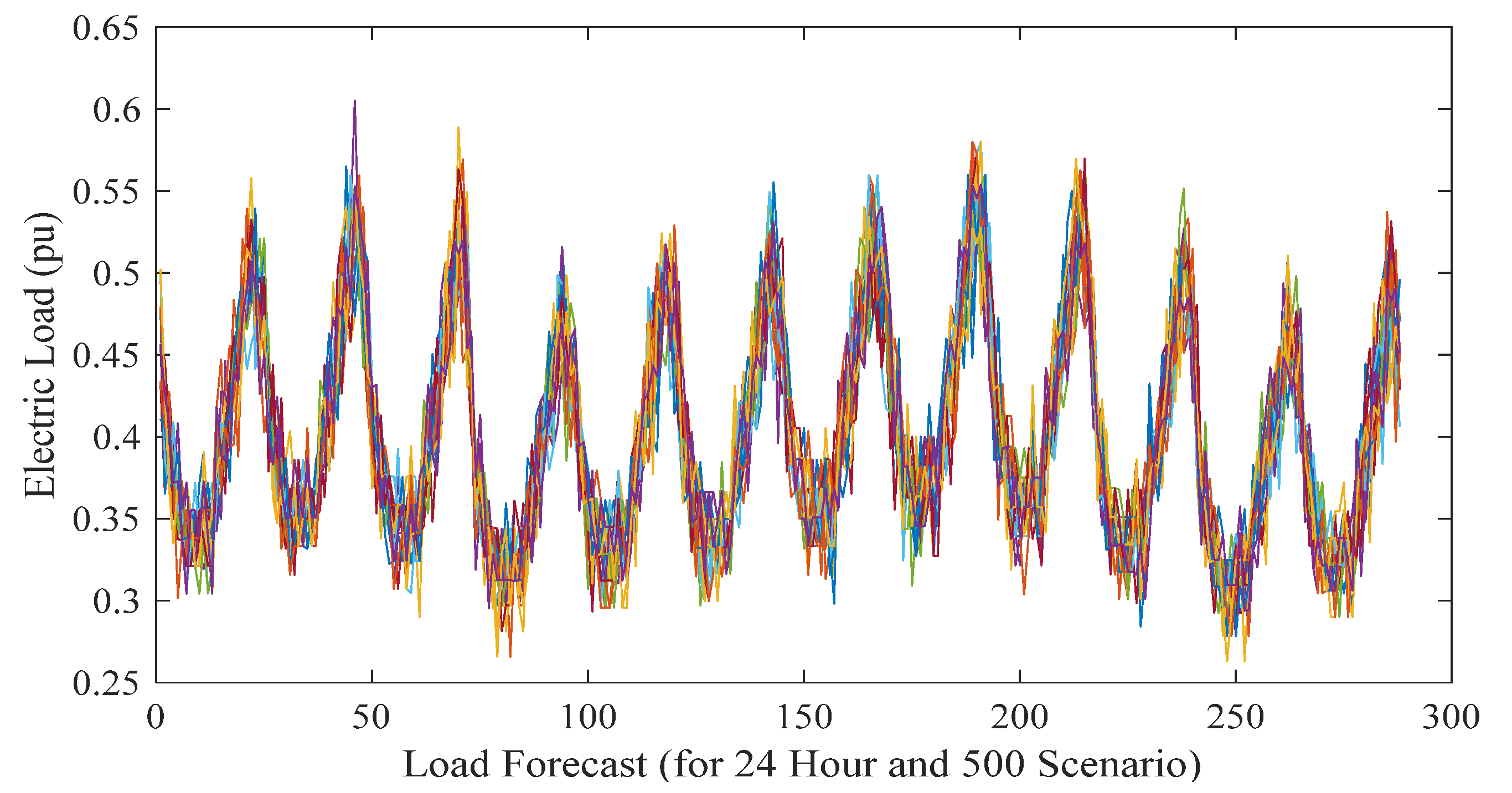
2.1. Load Uncertainty
2.2. Electricity Price Uncertainty
2.3. Electric Vehicle Charging Station
2.4. Wind Turbine
2.5. Photovoltaic System
2.6. Combined Hydrogen, Heat, and Power (CHHP)
2.6.1. Electrolyzer
2.6.2. Fuel Cell
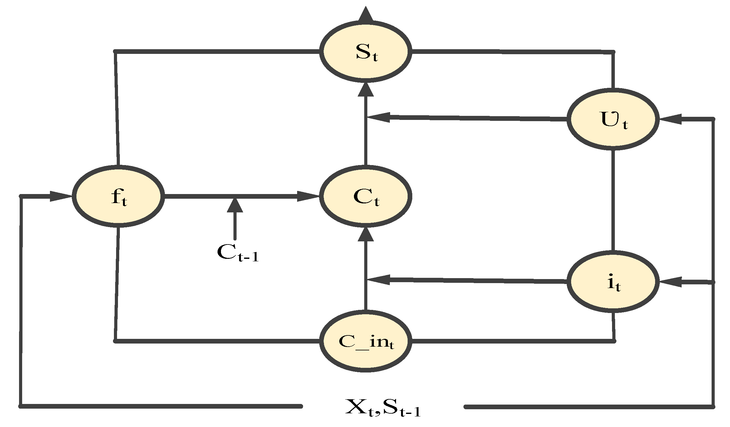
2.7. LSTM Model
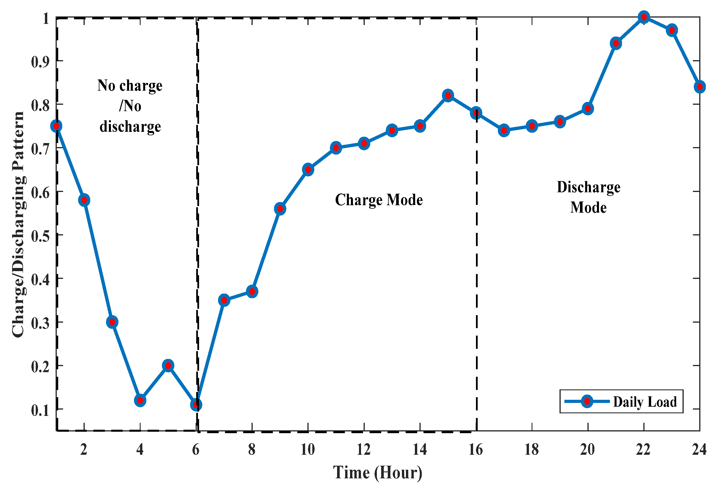
2.8. Demand Response
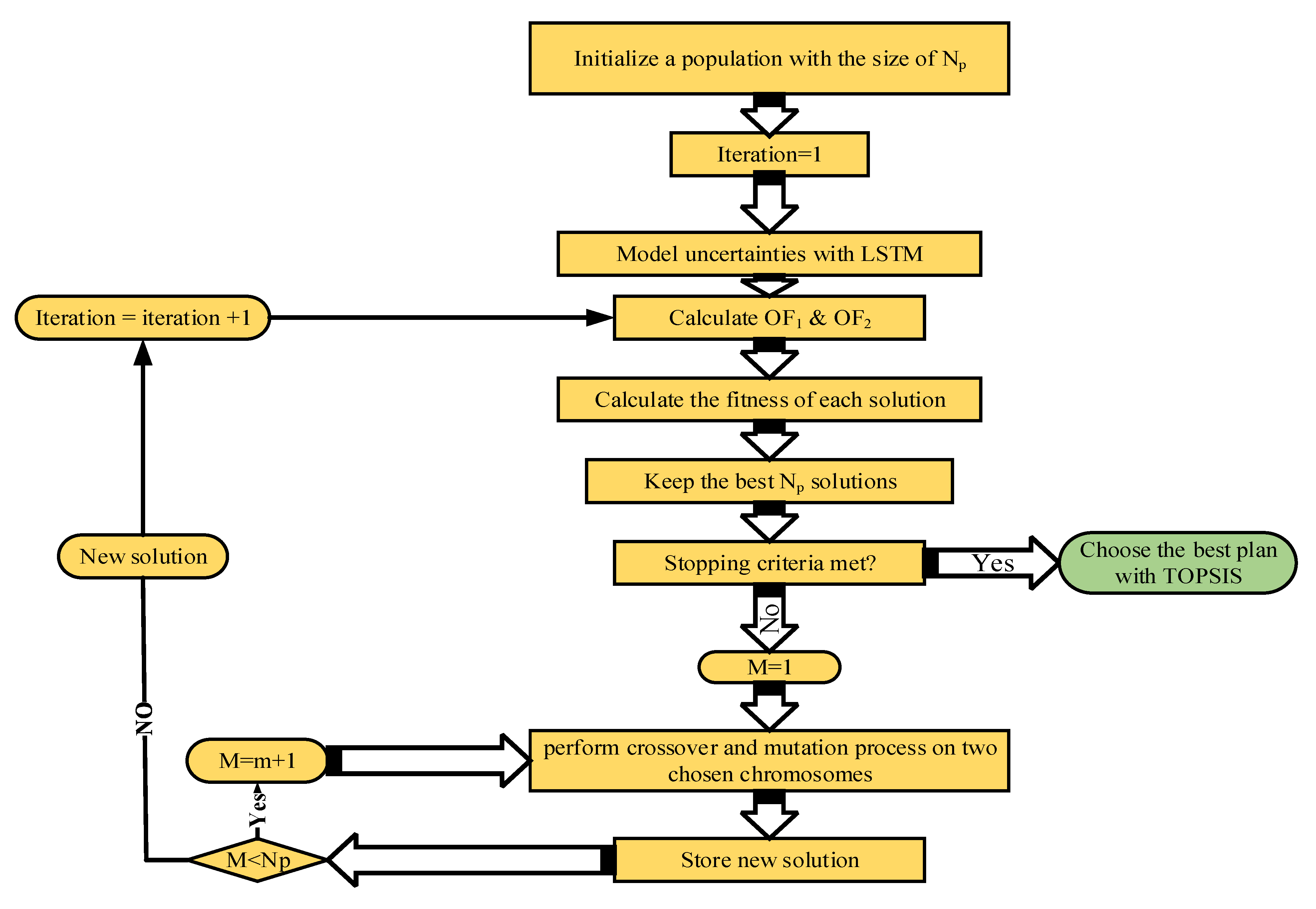
3. Problem-Solving Algorithm
4. Results
4.1. Input Data
4.2. Numerical Results
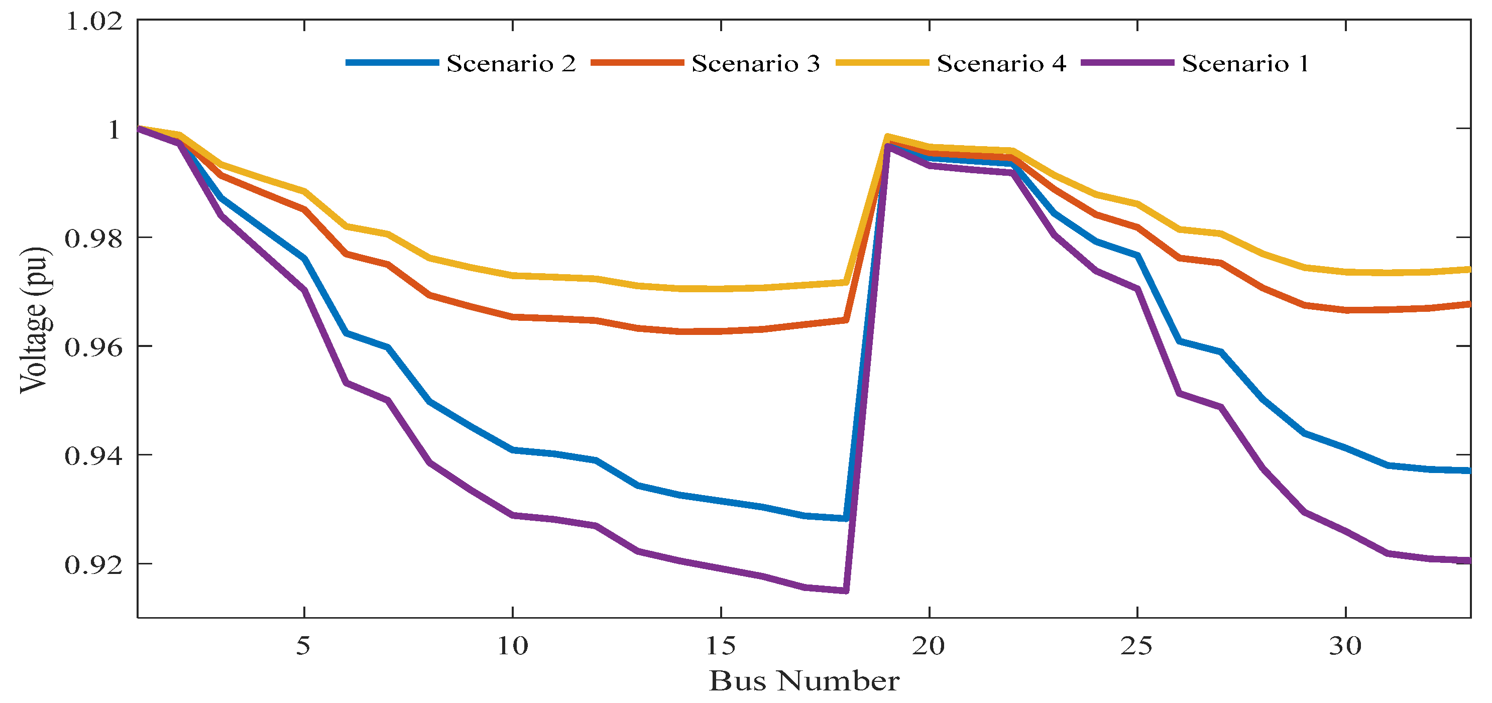
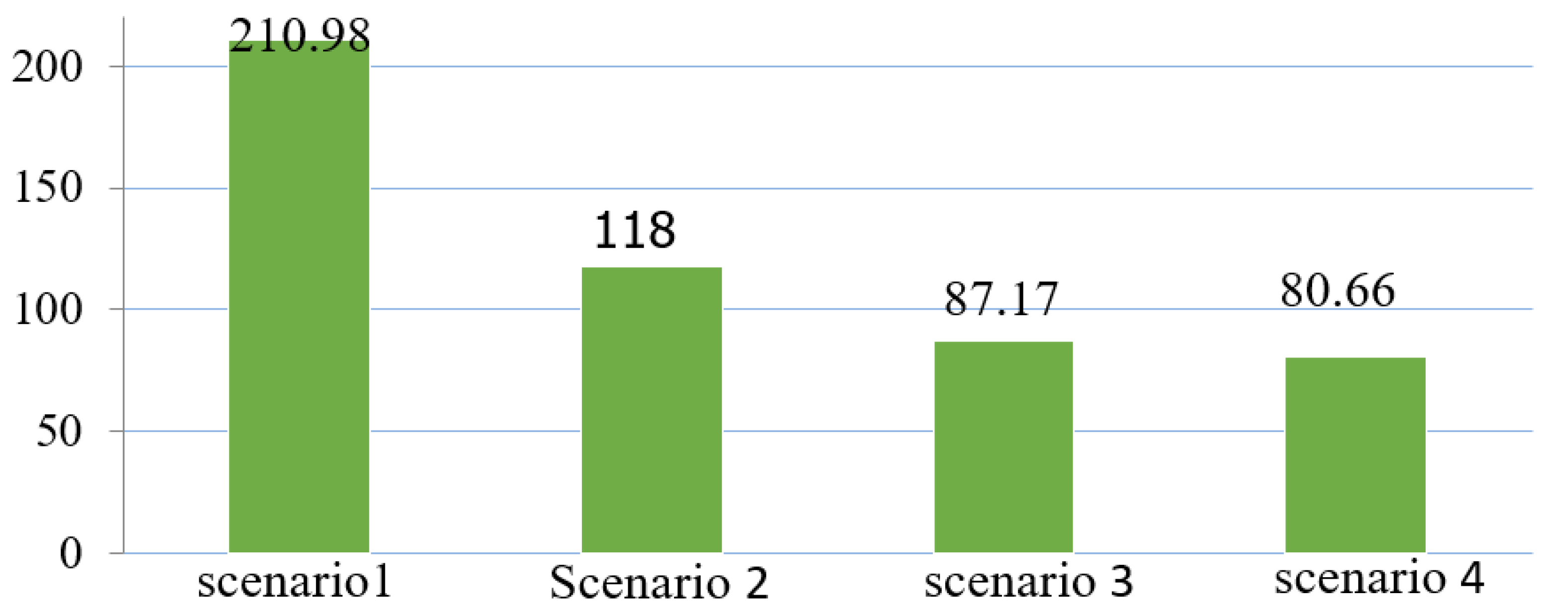
- Scenario 1: Base state;
- Scenario 2: Optimal location of one SPL-CHHP and three SMs;
- Scenario 3: Optimal location of two SPL-CHHP and three SMs;
- Scenario 4: Optimal location of three SPL-CHHP and three SMs.
- Mode 1: location of the CHHP in single power factor mode, without locating the SMs;
- Mode 2: location of the CHHP in the adaptive power factor mode, without the presence of SMs;
- Mode 3: simultaneous location of CHHP in adaptive power factor mode and SMs.
4.3. TOPSIS Results
4.4. Comparison with Other Techniques
5. Conclusions
Author Contributions
Funding
Conflicts of Interest
Nomenclature
| Indices | |
| CHHP index | |
| SPL index | |
| WT index | |
| WT index | |
| h | Electrolyzer index |
| Fuel cell index | |
| Time index | |
| k | Index related to branches |
| Parameters | |
| OF1 | First objective function |
| OF2 | Second objective function |
| Ploss | Active power loss (kW) |
| Voltage of bus n at time t | |
| Voltage of bus m at time t | |
| Vi | Voltage of bus i |
| Voltage drop index | |
| Total installation cost of CHHP ($) | |
| Total installation cost of the smart parking lot ($) | |
| Total operational cost (S) | |
| Total emissions cost (S) | |
| Price of purchased electricity ($/kWh) | |
| Amount of purchased power from the main grid (kW) | |
| Output power of the SPL (kW) | |
| Output power of CHHP (kW) | |
| Amount of power produced by WT (kW) | |
| Amount of power produced by PV (kW) | |
| Emissions per kWh from CHHP (kg/kW) | |
| Emissions per kWh from SPL (kg/kW) | |
| Emissions per kWh from UG (kg/kW) | |
| Load growth at time t | |
| Base complex power (kVA) | |
| Base reactive power (kVar) | |
| Variance of price prediction | |
| Price of purchased energy from the main grid ($/kWh) | |
| State of charge variance | |
| Variance in the EV’s arrival at the SPL | |
| Variance in the EV’s departure from the SPL | |
| Hydrogen exchange at time t | |
| Capacity of heat storage | |
| Binary value to show outflow heat energy | |
| Weight of xi | |
| Weight of xo | |
| Input variable at time t | |
| Weight of ho | |
| State at time t−1 | |
| EV’s state of charge at time t | |
| EV’s discharge efficiency | |
| EV’s charge efficiency | |
| Mean value of price prediction | |
| Initial value of SOC | |
| Mean value of SOC prediction | |
| Maximum value of initial SOC | |
| Minimum value of initial SOC | |
| Time of discharged power | |
| Time of charging power | |
| Binary variable of charging mode | |
| Binary variable of discharging mode | |
| Charging power of EV (kW) | |
| Discharging power of EV (kW) | |
| Cut-out velocity of the WT (m/s) | |
| Rated velocity of the WT (m/s) | |
| Efficiency of converting irradiation to electricity in the PV | |
| Surface of the PV cell | |
| Ambient temperature | |
| Absorbed irradiation | |
| Probabilistic distribution of the Ir | |
| Parameters of the sun irradiation prediction PDF | |
| Efficiency of the electrolyzer | |
| Efficiency of the fuel cell | |
| Heat storage efficiency | |
| Efficiency of transferring thermal energy |
References
- Zhang, X.; Shahidehpour, M.; AlAbdulwahab, A.; Abusorrah, A. Optimal expansion planning of energy hub with multiple energy infrastructures. IEEE Trans. Smart Grid 2015, 6, 2302–2311. [Google Scholar] [CrossRef]
- Morvaj, B.; Evins, R.; Carmeliet, J. Optimizing urban energy systems: Simultaneous system sizing, operation and district heating network layout. Energy 2016, 116, 619–636. [Google Scholar] [CrossRef]
- Coelho, B.; Andrade-Campos, A. Energy recovery in water networks: Numerical decision support tool for optimal site and selection of micro turbines. J. Water Resour. Plan. Manag. 2018, 144, 04018004. [Google Scholar] [CrossRef]
- Delfino, F.; Ferro, G.; Minciardi, R.; Robba, M.; Rossi, M.; Rossi, M. Identification and optimal control of an electrical storage system for microgrids with renewables. Sustain. Energy Grids Netw. 2019, 17, 100183. [Google Scholar] [CrossRef]
- Rostami, R.; Hosseinnia, H. Impacts of Contributing Distribution Network Operator (DNO) and Distributed Generation Unit Operator (DGO) in Benefit Maximizing. In Proceedings of the 7th Iran Wind Energy Conference (IWEC2021), Shahrood, Iran, 17–18 May 2021; pp. 1–4. [Google Scholar]
- Hosseinnia, H.; Nazarpour, D.; Talavat, V. Benefit maximization of demand side management operator (DSMO) and private investor in a distribution network. Sustain. Cities Soc. 2018, 40, 625–637. [Google Scholar] [CrossRef]
- Thirugnanam, K.; Kerk, S.K.; Yuen, C.; Liu, N.; Zhang, M. Energy management for renewable microgrid in reducing diesel generators usage with multiple types of battery. IEEE Trans. Ind. Electron. 2018, 65, 6772–6786. [Google Scholar] [CrossRef]
- Gbadamosi, S.; Nwulu, N.I. Optimal power dispatch and reliability analysis of hybrid CHP-PV-wind systems in farming applications. Sustainability 2020, 12, 8199. [Google Scholar] [CrossRef]
- Misconel, S.; Zöphel, C.; Möst, D. Assessing the value of demand response in a decarbonized energy system–A large-scale model application. Appl. Energy 2021, 299, 117326. [Google Scholar] [CrossRef]
- Duman, A.C.; Erden, H.S.; Gönül, Ö.; Güler, Ö. A home energy management system with an integrated smart thermostat for demand response in smart grids. Sustain. Cities Soc. 2021, 65, 102639. [Google Scholar] [CrossRef]
- Abdelaziz, M. GPU-OpenCL accelerated probabilistic power flow analysis using Monte-Carlo simulation. Electr. Power Syst. Res. 2017, 147, 70–72. [Google Scholar] [CrossRef]
- Qin, B.; Fang, C.; Ma, K.; Li, J. Probabilistic energy flow calculation through the nataf transformation and point estimation. Appl. Sci. 2019, 9, 3291. [Google Scholar] [CrossRef] [Green Version]
- Said, S.M.; Ali, A.; Hartmann, B. Tie-line power flow control method for grid-connected microgrids with SMES based on optimization and fuzzy logic. J. Mod. Power Syst. Clean Energy 2020, 8, 941–950. [Google Scholar] [CrossRef]
- Wei, X.; Xie, Z.; Cheng, R.; Zhang, D.; Li, Q. An Intelligent Learning and Ensembling Framework for Predicting Option Prices. Emerg. Mark. Financ. Trade 2020, 12, 1–24. [Google Scholar] [CrossRef]
- Shivaie, M.; Kiani-Moghaddam, M.; Weinsier, P.D. Bilateral bidding strategy in joint day-ahead energy and reserve electricity markets considering techno-economic-environmental measures. Energy Environ. 2021, 6, 0958305X211014875. [Google Scholar]
- Giap, V.-T.; Lee, Y.D.; Kim, Y.S.; Ahn, K.Y. A novel electrical energy storage system based on a reversible solid oxide fuel cell coupled with metal hydrides and waste steam. Appl. Energy 2020, 262, 114522. [Google Scholar] [CrossRef]
- Singh, S.; Chauhan, P.; Singh, N. Capacity optimization of grid connected solar/fuel cell energy system using hybrid ABC-PSO algorithm. Int. J. Hydrog. Energy 2020, 45, 10070–10088. [Google Scholar] [CrossRef]
- Sorlei, I.-S.; Bizon, N.; Thounthong, P.; Varlam, M.; Carcadea, E.; Culcer, M.; Iliescu, M.; Raceanu, M. Fuel cell electric vehicles—A brief review of current topologies and energy management strategies. Energy 2021, 14, 252. [Google Scholar]
- Mohseni, S.; Brent, A.C.; Burmester, D.; Browne, W.N. Lévy-flight moth-flame optimisation algorithm-based micro-grid equipment sizing: An integrated investment and operational planning approach. Energy AI 2021, 3, 100047. [Google Scholar] [CrossRef]
- Suresh, M.; Meenakumari, R. Optimum utilization of grid connected hybrid renewable energy sources using hybrid algorithm. Trans. Inst. Meas. Control 2021, 43, 21–33. [Google Scholar] [CrossRef]
- Bahmani, R.; Karimi, H.; Jadid, S. Stochastic electricity market model in networked microgrids considering demand response programs and renewable energy sources. Int. J. Electr. Power Energy Syst. 2020, 117, 105606. [Google Scholar] [CrossRef]
- Arévalo, P.; Tostado-Véliz, M.; Jurado, F. A novel methodology for comprehensive planning of battery storage systems. J. Energy Storage 2021, 37, 102456. [Google Scholar] [CrossRef]
- Tostado-Véliz, M.; Icaza-Alvarez, D.; Jurado, F. A novel methodology for optimal sizing photovoltaic-battery systems in smart homes considering grid outages and demand response. Renew. Energy 2021, 170, 884–896. [Google Scholar] [CrossRef]
- Khasanov, M.; Kamel, S.; Rahmann, C.; Hasanien, H.M.; Al-Durra, A. Optimal distributed generation and battery energy storage units integration in distribution systems considering power generation uncertainty. IET Gener. Transm. Distrib. 2021, 2, 1–23. [Google Scholar]
- Ahrabi, M.; Abedi, M.; Nafisi, H.; Mirzaei, M.A.; Mohammadi-Ivatloo, B.; Marzband, M. Evaluating the effect of electric vehicle parking lots in transmission-constrained AC unit commitment under a hybrid IGDT-stochastic approach. Int. J. Electr. Power Energy Syst. 2021, 125, 106546. [Google Scholar] [CrossRef]
- Kong, X.; Liu, D.; Wang, C.; Sun, F.; Li, S. Optimal operation strategy for interconnected microgrids in market environment considering uncertainty. Appl. Energy 2020, 275, 115336. [Google Scholar] [CrossRef]
- Cai, S.; Xie, Y.; Wu, Q.; Xiang, Z. Robust MPC-based microgrid scheduling for resilience enhancement of distribution system. Int. J. Electr. Power Energy Syst. 2020, 121, 106068. [Google Scholar] [CrossRef]
- Shi, Q.; Li, F.; Olama, M.; Dong, J.; Xue, Y.; Starke, M.; Winstead, C.; Kuruganti, T. Network Reconfiguration and Distributed Energy Resource Scheduling for Improved Distribution System Resilience. Int. J. Electr. Power Energy Syst. 2021, 124, 106355. [Google Scholar] [CrossRef]
- Zhou, M.; Wu, Z.; Wang, J.; Li, G. Forming dispatchable region of electric vehicle aggregation in microgrid bidding. IEEE Trans. Ind. Inform. 2020, 17, 4755–4765. [Google Scholar] [CrossRef]
- Ebrahimi, J.; Abedini, M.; Rezaei, M.M.; Nasri, M. Optimum design of a multi-form energy in the presence of electric vehicle charging station and renewable resources considering uncertainty. Sustain. Energy Grids Netw. 2020, 23, 100375. [Google Scholar] [CrossRef]
- Ghotge, R.; Snow, Y.; Farahani, S.; Lukszo, Z.; Van Wijk, A. Optimized scheduling of EV charging in solar parking lots for local peak reduction under EV demand uncertainty. Energies 2020, 13, 1275. [Google Scholar] [CrossRef] [Green Version]
- Langenmayr, U.; Wang, W.; Jochem, P. Unit commitment of photovoltaic-battery systems, An advanced approach considering uncertainties from load, electric vehicles, and photovoltaic. Appl. Energy 2020, 280, 115972. [Google Scholar] [CrossRef]
- Okpokparoro, S.; Sriramula, S. Uncertainty modeling in reliability analysis of floating wind turbine support structures. Renew. Energy 2021, 165, 88–108. [Google Scholar] [CrossRef]
- Luo, L.; Abdulkareem, S.S.; Rezvani, A.; Miveh, M.R.; Samad, S.; Aljojo, N.; Pazhoohesh, M. Optimal scheduling of a renewable based microgrid considering photovoltaic system and battery energy storage under uncertainty. J. Energy Storage 2020, 28, 101306. [Google Scholar] [CrossRef]
- Gül, M.; Akyüz, E. Hydrogen generation from a small-scale solar photovoltaic thermal (PV/T) electrolyzer system: Numerical model and experimental verification. Energies 2020, 13, 2997. [Google Scholar] [CrossRef]
- Van Houdt, G.; Mosquera, C.; Nápoles, G. A review on the long short-term memory model. Artif. Intell. Rev. 2020, 53, 5929–5955. [Google Scholar] [CrossRef]
- Tostado-Véliz, M.; Bayat, M.; Ghadimi, A.A.; Jurado, F. Home energy management in off-grid dwellings: Exploiting flexibility of thermostatically controlled appliances. J. Clean. Prod. 2021, 310, 127507. [Google Scholar] [CrossRef]
- Kirkerud, J.G.; Nagel, N.O.; Bolkesjø, T.F. The role of demand response in the future renewable northern European energy system. Energy 2021, 235, 121336. [Google Scholar] [CrossRef]


| Unit | CHHP | PV | PL | Other Data | ||||||||||
|---|---|---|---|---|---|---|---|---|---|---|---|---|---|---|
| Parameter | S | If | Ir | (year) | ||||||||||
| Value | 0.7 | 0.85 | 0.80 | 12.5% | 800 | 25 | 0.90 | 0.81 | 0 | 8–22% | 10% | 10% | 10 | 3% |
| TOU Program | Fuel Cell | WT | |||||
|---|---|---|---|---|---|---|---|
| Peak | Normal | Low | |||||
| 20–23 | 7:00–19:59 | 0:00–6:59 | |||||
| 0.52($/kWh) | 0.40($/kWh) | 0.25($/kWh) | 0.80 | 5 | 15 | 12 | 11 |
| Scenario | Case | Minimum Voltage (p.u.) | Power Loss Reduction | Total Cost (*106) | Optimal Site and Size of DGs | Optimal pf |
|---|---|---|---|---|---|---|
| Scenario 1 | Base Mode | 0.9038 | ‒ | ‒ | ‒ | ‒ |
| B(18) | ||||||
| Scenario 2 | Case 1 | 0.9276 | 44.07 | 1.052 | 1.875(B8) | 1 |
| B(33) | ||||||
| Case 2 | 0.9481 | 60.6 | 1.048 | 1.889(B8) | 0.85(B8) | |
| B(33) | ||||||
| Scenario 3 | Case 1 | 0.9586 | 58.68 | 1.030 | 0.905(B13) | 1.00(B13) |
| B(31) | 1.012(B30) | 1.00(B30) | ||||
| Case 2 | 0.9724 | 80.6 | 1.012 | 0.808(B16) | 0.84(B16) | |
| B(25) | 1.089(B30) | (B30)0.91 | ||||
| Scenario 4 | Case 1 | 0.9502 | 61.77 | 1.001 | (B14)0.799 | 1.00(B14) |
| 1.00(B25) | ||||||
| B(31) | 1.00(B31) | |||||
| Case 2 | 0.9475 | 86.33 | 0.985 | 0.91(B14) | 0.579(B14) | |
| B(25) | 0.9(B25) | 0.847(B25) | ||||
| 0.85(B30) | 0.378(B30) |
| Scenario | Mode | Total Cost (*106$) | Minimum Voltage | Site & Size of DG | Site of SM |
|---|---|---|---|---|---|
| 1 | Base | 0.992 | 0.9038 | ‒ | ‒ |
| (B18) | |||||
| 2 | 1 | 1.628 | 0.9389 | 1.75.0(B12) | ‒ |
| B(33) | |||||
| 2 | 1.702 | 0.9537 | 1.856(B8) | ‒ | |
| B(33) | |||||
| 3 | 0.9205(B33) | 0.9548 | 1.890(B8) | B6, B25, B30, | |
| B(33) | B31, B32 | ||||
| 3 | 1 | 0.9115(B31) | 0.9618 | 1.352(B14) | ‒ |
| B(31) | 0.623(B33) | ||||
| 2 | 0.9826(B25) | 0.9689 | 0.988(B17) | ‒ | |
| B(25) | 1.011(B33) | ||||
| 3 | 0.9825(B33) | 0.9745 | 0.953(B14) | B7, B14, B18, B20, B32 | |
| B(33) | 1.042(B32) | ||||
| 4 | 1 | 0.9578 (B31) | 0.9678 | 0.959(B13) | ‒ |
| B(31) | 0.507(B16) | ||||
| 0.534(B33) | |||||
| 2 | 0.9512(B25) | 0.9759 | 0.719(B15) | ‒ | |
| B(25) | 0.417(B18) | ||||
| 0.862(B33) | |||||
| 3 | 0.9610(B25) | 0.9785 | 0.700(B15) | B8, B29, B30, B31, B32 | |
| B(25) | 0.430(B18) | ||||
| 0.870(B28) |
| Function and Scenario | OF1: Voltage Drop Index | Function and Scenario | OF2: Minimizing Cost Function | ||||
|---|---|---|---|---|---|---|---|
| Mode | VDI | CF (*106$) | Mode | CF (*106$) | VDI | ||
| OF1 Scenario2 | 1 | 0.0332 | 1.0289 | OF2 Scenario2 | 1 | 1.0204 | 0.0185 |
| 2 | 0.0128 | 1.0119 | 2 | 1.0100 | 0.0110 | ||
| 3 | 0.0112 | 1.0101 | 3 | 1.0098 | 0.0102 | ||
| OF1 Scenario 3 | 1 | 0.0189 | 1.0126 | OF2 Scenario 3 | 1 | 1.0179 | 0.0152 |
| 2 | 0.0025 | 1.0012 | 2 | 1.0096 | 0.0062 | ||
| 3 | 0.0021 | 1.0009 | 3 | 1.0021 | 0.0032 | ||
| OF1 Scenario 4 | 1 | 0.0248 | 1.0158 | OF2 Scenario 4 | 1 | 1.0178 | 0.0128 |
| 2 | 0.0058 | 1.0092 | 2 | 1.0035 | 0.0039 | ||
| 3 | 0.0025 | 1.0029 | 3 | 1.0019 | 0.0020 | ||
| Method | Number of Pareto Optimal Solutions | Running Time(s) | ||||
|---|---|---|---|---|---|---|
| GA + AHP | 12 | 0.2401 | 2.905 | 0.2011 | 3.899 | 28,564 |
| GA + ε-constraints | 16 | 0.3057 | 3.784 | 0.2089 | 3.6746 | 27,489 |
| GA + TOPSIS | 10 | 0.103 | 3.985 | 0.0725 | 4.717 | 18,705 |
Publisher’s Note: MDPI stays neutral with regard to jurisdictional claims in published maps and institutional affiliations. |
© 2021 by the authors. Licensee MDPI, Basel, Switzerland. This article is an open access article distributed under the terms and conditions of the Creative Commons Attribution (CC BY) license (https://creativecommons.org/licenses/by/4.0/).
Share and Cite
Hosseinnia, H.; Mohammadi-Ivatloo, B.; Mohammadpourfard, M. Optimal Techno-Economic Planning of a Smart Parking Lot—Combined Heat, Hydrogen, and Power (SPL-CHHP)-Based Microgrid in the Active Distribution Network. Appl. Sci. 2021, 11, 8043. https://doi.org/10.3390/app11178043
Hosseinnia H, Mohammadi-Ivatloo B, Mohammadpourfard M. Optimal Techno-Economic Planning of a Smart Parking Lot—Combined Heat, Hydrogen, and Power (SPL-CHHP)-Based Microgrid in the Active Distribution Network. Applied Sciences. 2021; 11(17):8043. https://doi.org/10.3390/app11178043
Chicago/Turabian StyleHosseinnia, Hamed, Behnam Mohammadi-Ivatloo, and Mousa Mohammadpourfard. 2021. "Optimal Techno-Economic Planning of a Smart Parking Lot—Combined Heat, Hydrogen, and Power (SPL-CHHP)-Based Microgrid in the Active Distribution Network" Applied Sciences 11, no. 17: 8043. https://doi.org/10.3390/app11178043