Article

Rotational Speed Control Using ANN-Based MPPT for OWC Based on Surface Elevation Measurements

1
Automatic Control Group—ACG, Institute of Research and Development of Processes—IIDP, Department of Automatic Control and Systems Engineering, Faculty of Engineering of Bilbao, University of the Basque Country—UPV/EHU, Po Rafael Moreno no3, 48013 Bilbao, Spain
2
Automatic Control Group—ACG, Institute of Research and Development of Processes—IIDP, Department of Electricity and Electronics, Faculty of Science and Technology, University of the Basque Country—UPV/EHU, Bo Sarriena s/n, 48080 Leioa, Spain
*
Author to whom correspondence should be addressed.
Appl. Sci. 2020, 10(24), 8975; https://doi.org/10.3390/app10248975
Submission received: 13 October 2020 / Revised: 7 December 2020 / Accepted: 12 December 2020 / Published: 16 December 2020
(This article belongs to the Special Issue Modeling, Design and Control of Electric Machines)

Abstract

:
This paper presents an ANN-based rotational speed control to avoid the stalling behavior in Oscillating Water Columns composed of a Doubly Fed Induction Generator driven by a Wells turbine. This control strategy uses rotational speed reference provided by an ANN-based Maximum Power Point Tracking. The ANN-based MPPT predicts the optimal rotational speed reference from wave amplitude and period. The neural network has been trained and uses wave surface elevation measurements gathered by an acoustic Doppler current profiler. The implemented ANN-based rotational speed control has been tested with two different wave conditions and results prove the effectiveness of avoiding the stall effect which improved the power generation.

1. Introduction

Global energy transformation is the key to reduce climate damages. This transformation would help achieve a cheaper renewable power, reduction of emissions and air pollution, and increase welfare and growth. The World Meteorological Organization declared that the 20 hottest years recorded have all transpired during the last 22 years and the highest four took place in the last four years only [1]. In fact, the IPCC special report on the impacts of global warming of 1.5 °C states that during the latest decade (2009–2018) the average temperature was about 0.93 °C more than the pre-industrial baseline, and during the five years (2014–2018) it was 1.04 °C more than the baseline [2]. For these reasons, many efforts have been invested to reduce the damages of the climate change which can be seen in the objectives set by the Kyoto Protocol (1997) to decrease polluting emissions of five greenhouse gases (GHG); methane, nitrogen oxide, hydrofluorocarbons, perfluorocarbons, sulfur hexafluoride aside from the carbon dioxide to a minimum of 5% against the emissions documented in 1985 [3], and later with the objectives set by the 20-20-20 agenda which states that every European Country needs to achieve by 2020 a 20% emission level decrease on GHG from the 1990 numbers, a 20% renewables in the final energy consumption, and a 20% improvement of energy efficiency [4].
Despite these efforts, the average energy that are related to CO2 releases have escalated 1.3% yearly in the past five years widening the gap between registered emissions and the required emissions levels to reach the globally fixed climate goals [5]. Considering the accelerating climate change damages, the transformation of the global energy system requires significant acceleration to reach the goals of the Paris Agreement [6]. Those goals consist of keeping the increase in average global temperatures lower than 2 °C and preferably to restrict warming to 1.5 °C during this century.
Electrification based on renewables while combined with energy efficiency is the key ingredient of a successful energy transition that can guarantee a lower overall energy demand. This concept can start to reduce energy-related CO2 emissions immediately and substantially. Moreover, it decreases air pollution and raises health benefits, beneficial socio-economic advantages and can turn into an important factor to form a connected and digitalized economy and society. In this sense, governments should enforce further forceful climate, renewable energy and energy efficiency strategies and goals. Notably, governments ought to line up climate and sustainability objectives with power plans [5].
To fulfill the Paris Agreement on Climate Change, the Ocean Energy Forum established a strategic roadmap to build an ocean energy system for Europe which will guarantee around 10% of power demands of Europe through wave and tidal energy by 2050 [7]. The roadmap highlights the importance of Research and Development to speed up testing and validation of numerous ocean technologies to achieve a commercial maturity and secure industrial deployment [7]. According to the European Marine Energy Centre, many countries have been engaged in projects which concentrate on the development of the Wave Energy Converter (WEC) industry for instance United Kingdom (26 projects), Norway (14), Denmark (9), Spain (9), Ireland (7), Sweden (5), France (4), Finland-Germany-Portugal (2), and Greece (1) [8]. However, since many countries, which are developing WECs, are at various phase of development there exist no mutual ground to define the best configuration, Power Take-Off (PTO) system and control strategies in light of implementation intricacies. Hence, the central point of research, in next years, must change from large scale WECs to the difficulties of developing WECs and adapted projects proper to promote the development of niche markets [9].
The Oscillating Water Columns (OWC) are widely deployed wave energy converters thanks to their simplicity and feasibility. Nevertheless, OWC devices using Wells turbine-based PTO systems withstand a hindrance in power generation caused by the stalling phenomenon that affects the Wells turbine’s aerodynamic efficiency resulting into a reduced energy extraction [10,11]. Many scientists and research groups have studied and investigated the effects of the stalling phenomenon in Wells turbine and how to reduce its impact on the produced power. M. Toressi et al. worked on the stall effect of Wells turbine and performed many analyses from numerical and experimental data. In [12] they used detailed CFD to investigate the flow-field through the turbine blades to offer a description of the complex flow mechanism that originates separation and, consequently, low efficiency at high flowrates by solving the Reynolds-averaged Navier–Stokes equations together with three turbulence models. In addition, in [13] they investigated a 3D-printed Wells turbine in the open wind tunnel of the Polytechnic University of Bari. The scaled prototype was designed to operate in a 1:10 scaled model of a REWEC3 breakwater for ocean application and was tested under steady-state and pulsating flow conditions. Obtained results indicated that when the turbine experiences large sinusoidal variations of the flow coefficient at high mass flow rates, a delayed onset of stall can be observed and that the variation of the turbine performance under dynamic flow conditions is crucial for a correct design of the Wells turbine. F. Cambuli et al. investigated in [14] the dynamic interaction between the OWC and the Wells turbine. In this work, a lumped parameter model has been introduced and compared to experimental and CFD data. The proposed lumped parameter model allows rapid isolation of parameters with the largest influence on system performance and could be integrated with existing wave-to-wire models to improve the understanding of the hydrodynamic/aerodynamic interaction in the overall system. I. Hashem et al. investigated in [15] the possibility of enhancing the Wells turbine performance by using water as the working fluid rather than air by submerging the Wells turbine in the sea water. For this CFD simulations were performed using the steady 3D incompressible Reynolds-Averaged Navier–Stokes (RANS) calculations on this type of axial turbine rotor with realizable k- ε turbulence model. Also, from a control point of view, O. Barambones et al. proposed in [16] a real-time sliding mode control for a wave energy converter based on a Wells turbine using Lyapunov stability theory to analyze its stability. The proposed control is tested first by means of simulations using MATLAB/Simulink and then using a real-time experimental platform based on a dSPACE DS1103 control board.
The present manuscript introduces the OWC’s model and proposes a rotational speed control. The propose of the rotational speed control is to help the turbo-generator evade the stalling behavior which will increase the power generation. For this purpose, an ANN-based rotational speed control has been developed and implemented with the intention to control the back-to-back (BTB) converter connected to a Doubly Fed Induction Generator (DFIG). This will allow the regulation of the rotational speed by considering the wave input and predicting the optimal rotational speed via an Artificial Neural Network (ANN)-based Maximum Power Point Tracking (MPPT). The designed network has been trained using measured wave data from the harbor of Mutriku by means of an Acoustic Doppler Current Profiler (ADCP) and its capabilities have been adopted to recognize the incoming strong waves causing the stall effect and generate the suitable reference value of the desired rotational speed for the proposed rotational speed control scheme.
The rest of this manuscript is structured as follows: Section 2 presents the theoretical considerations of the OWC plant model, of the stalling phenomenon and the Artificial Neural Networks to be used. Section 3 explains the materials and methods used to carry out the design and development of the proposed ANN rotational speed control. Section 4 discusses the performance of the designed ANN-based MPPT and the selected model, it also sets two demonstrative study cases to study the effectiveness of the proposed ANN rotational speed control with regular waves and with real measured waves. Finally, Section 5 finishes the paper with some concluding remarks.

2. Theoretical Considerations

The work presented in this paper requires the understanding of the system to be controlled and the Artificial Neural Networks to be used. In this sense, this part introduces the modeling of the different parts constituting the studied Wave Energy Converter (WEC) which is the Oscillating Water Column (OWC) illustrated in Figure 1, this would include the mathematical models of the waves, capture chamber, Wells turbine and the generator. In addition, a brief background on the Artificial Neural Networks.

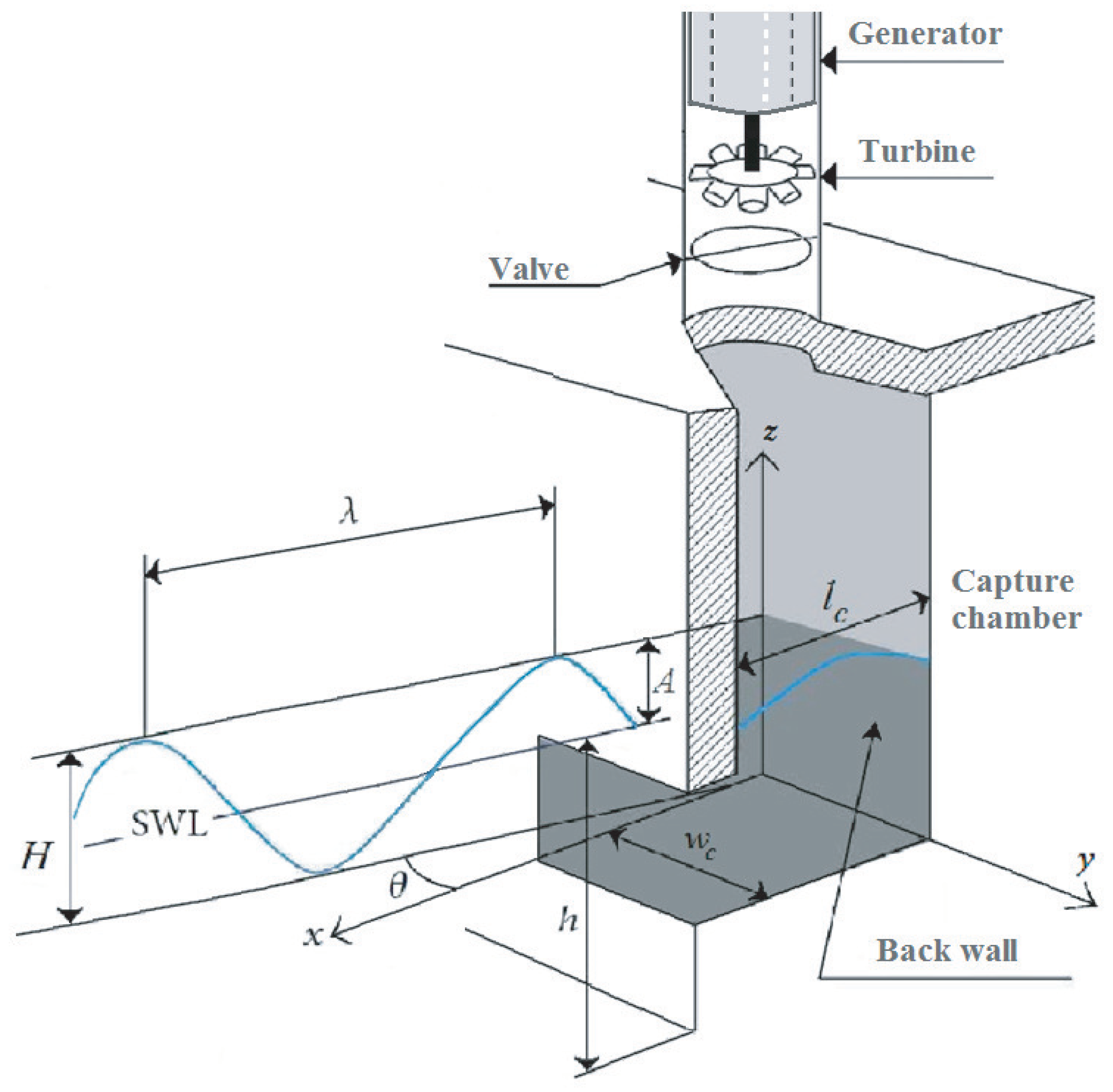
2.1. Wave Surface Dynamics

In the literature there exist many wave theories to describe the wave’s surface dynamics such as Cnoidal wave theory, second or higher-order Stokes theory and Airy linear theory [17,18]. For this work, monochromatic unidirectional wave has been considered to be input to the developed numerical wave-to-wire model of the OWC plant.
The Airy wave theory is the simplest depiction of waves, it describes the waves as sinusoidal waveforms by neglecting turbulences, friction losses and other energy losses [18].
The waveform of a regular wave is depicted in Figure 1, where S W L denotes the Still Water Level, h marks the sea depth between the seabed and the S W L . H represents the wave which is between the wave trough and the wave crest. A marks the wave amplitude which is between S W L and the wave crest and λ marks the wavelength which measures the distance between successive crests [18,19].
Therefore, the elevation of a wave’s surface can be expressed by [19,20]:
z ( x , t ) = A sin ω t k x θ = H / 2 sin ω t k x θ
here x represents the horizontal coordinate with the direction of wave propagation as positive direction, θ represents the angle between the x axis and the wave direction, and k represents the wave number defined by (2) given in [21].
k tanh ( k h ) = ω 2 / g
where ω is the wave frequency and g is the acceleration gravity.

2.2. Capture Chamber Model

The air volume in the capture chamber of the oscillating water column is defined from the chamber’s volume and the water volume as [20,21,22]:
V ( t ) = V c + w c H k sin k l c / 2 sin ( ω t )
where V c , w c and l c are respectively the capture chamber’s volume, inner width and length.
The volume flow rate can be defined from Equation (3) by [20,21,22]:
Q ( t ) = w c c H sin k l c 2 cos ( ω t )
with c = w c / k .
From the expression of the volume flow rate (4) and considering the geometry of the chamber, the airflow speed can be expressed by [20,21,22]:
v x ( t ) = Q ( t ) S = 8 A c w c π D 2 sin π l c c T w cos 2 π T w t
where D is the duct diameter, T w is the wave period.

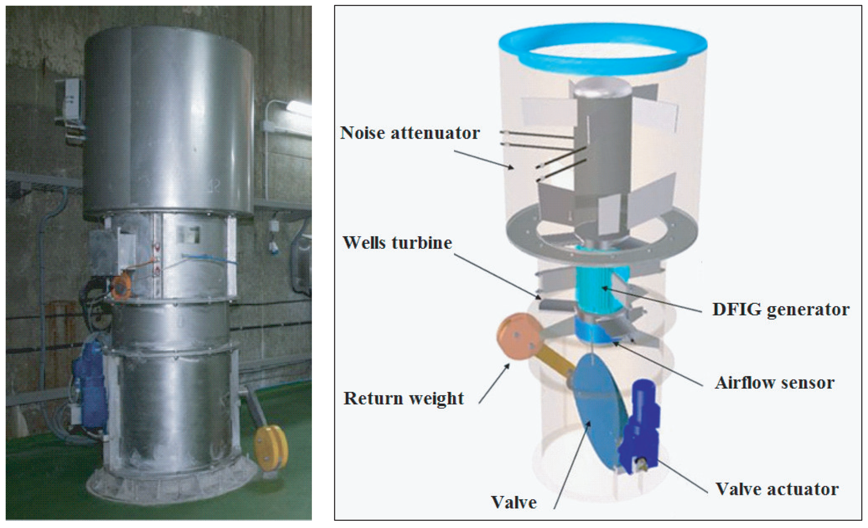
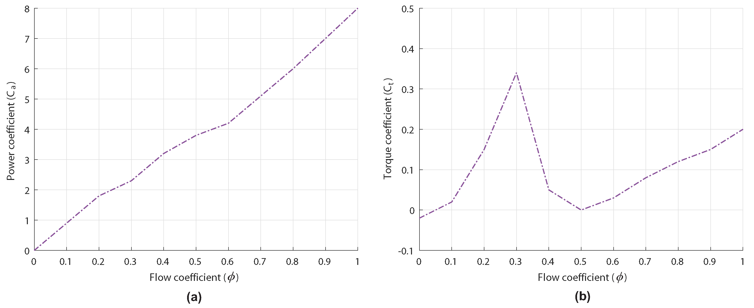
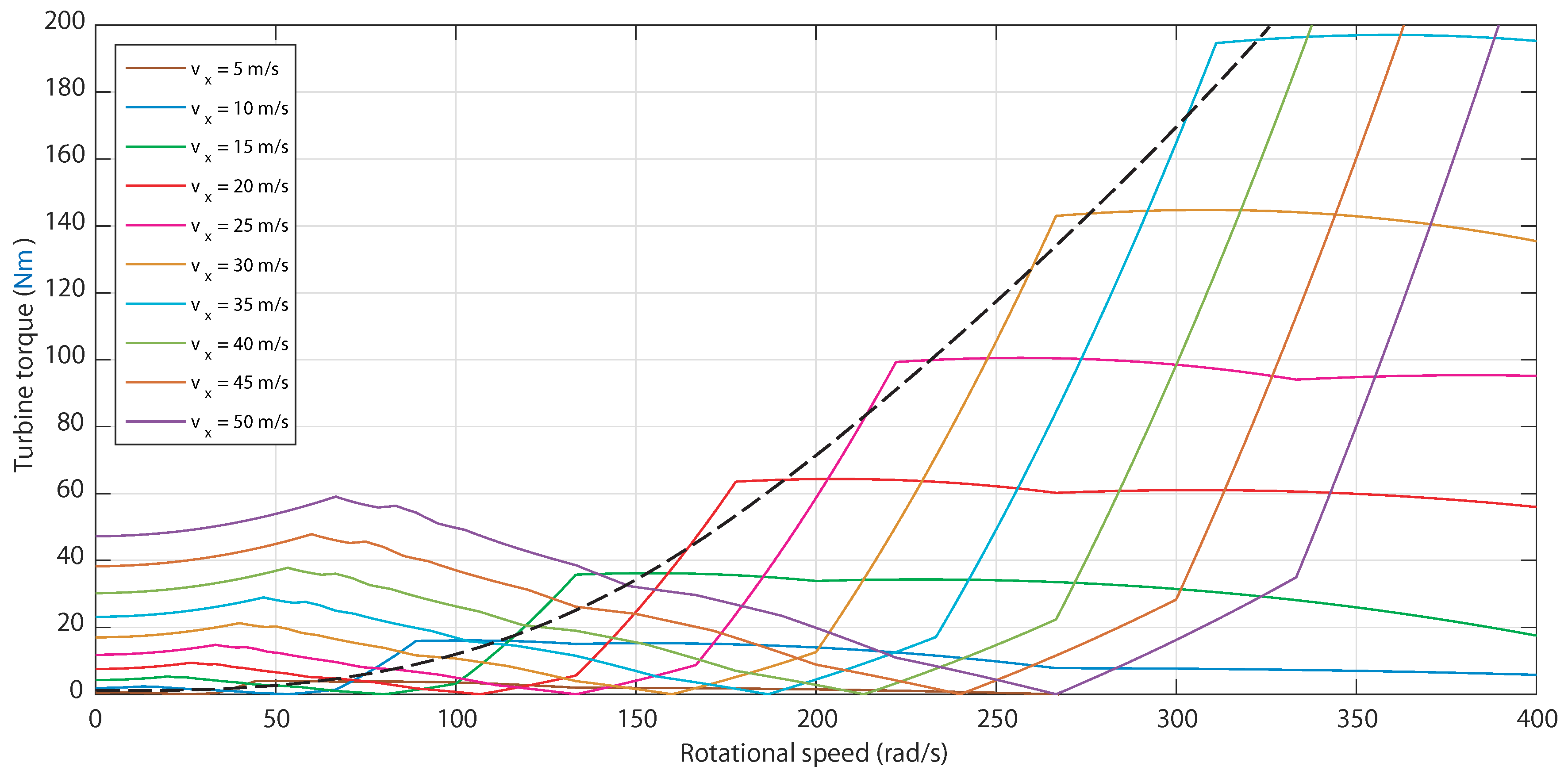
2.3. Wells Turbine Model

The considered air turbine is a Wells turbine which is a self-rectifying axial-flow turbine [23]. This type of air turbines permits a unidirectional pivotal motion unrelatedly to the airflow direction thanks to the blade’s distinct shape [24,25].
The Wells turbine shown in Figure 2 may be described by the equations given in [11] where the pressure drop across the turbine rotor is defined as:
d p = C a K 1 1 a a v x 2 + r ω r 2
where a is the cross-sectional area, C a is the power coefficient, r is the mean radius, ω r is the angular velocity.
The turbine constant K is different from Wells turbine to another and is obtained from the turbine’s geometry as:
K = ρ l b n 2
where ρ is the air density, l is the blade chord length, b is the blade height, and n is the number of blades.
The torque produced by the turbine will mainly depend on the turbine’s mechanical characteristics and both airflow and rotational speed which is expressed as:
T t = r C t K v x 2 + r ω r 2
where C t is the torque coefficient.
The relation between the torque and the pressure drop may be defined as:
T t = r a C t C a d p
The flow coefficient is obtained from the ratio of the airflow speed by rotational speed as:
ϕ = v x r ω r 1
The expression of the flow rate can be defined as a function of the cross-section area and the airflow speed as:
Q = a v x
Lastly, the turbine efficiency may be written as:
η t = T t ω r d p Q 1 = C t C a ϕ 1
The characteristic curves of the Wells turbine under steady-state operating conditions, for which no hysteretic loop is reported, are formed by the power coefficient C a and the torque coefficient C t versus the flow coefficient ϕ depicted in Figure 3.

2.4. Doubly Fed Induction Generator Model

The mathematical modeling of the Doubly Fed Induction Generator is defined by the expressions provided in [26,27]. The d q components of both the stator and rotor voltages are defined as:
v d s = R s i d s + d ψ d s d t ω s ψ q s v q s = R s i q s + d ψ q s d t + ω s ψ d s
v d r = R r i d r + d ψ d r d t ω r ψ q r v q r = R r i q r + d ψ q r d t + ω r ψ d r
with R s and R r are the stator and the rotor resistances, ω s and ω r are the stator and the rotor angular velocity, i d s and i q s are the d-q stator currents, i d r and i q r are the d-q rotor currents.
The d q components of the flux linkage are defined by:
ψ d s = L s s i d s + L m i d r ψ q s = L s s i q s + L m i q r
ψ d r = L r r i d r + L m i d s ψ q r = L r r i q r + L m i q s
with L s s and L r r are stator and rotor inductances and L m the magnetizing inductance.
The electromagnetic torque obtained from the DFIG is defined by:
T e = 3 2 p ψ d s i q s ψ q s i d s
with p is the pair pole number.
The mechanical interaction between the turbine and the generator can be defined as:
J p d ω r d t = T e T t
with J is the inertia of the system.

2.5. Back-to-Back Converter Model

The BTB converter is formed of a Grid-Side Converter (GSC) connected to the Grid and a Rotor-Side Converter (RSC) connected to the windings of the rotor in the DFIG [28].
The main role of the RSC is delivering voltage to the windings of the rotor in the DFIG. Its objective is aligning the rotor-flux with the stator-flux through the rotor-current control to obtain the required torque. Therefore, the RSC enables the stator voltages and generated power regulation [29].
The active and reactive powers across the stator are defined by [30,31]:
P s = 3 / 2 ( v d s i d s + v q s i q s )
Q s = 3 / 2 ( v q s i d s v d s i q s )
The grid voltages can be defined as:
v d g = R g i d g + L g d i d g d t ω g L g i q g + u d g v q g = R g i q g + L g d i q g d t + ω g L g i d g + u q g
where R g and L g are the grid coupling resistance and inductance, ω g is the grid’s angular frequency, i d g and i q g are the d-q grid currents and u d g and u q g are the GSC voltages.
The equations describing the active and reactive powers between the GSC and the Grid are:
P g = 3 / 2 ( v d g i d g + v q g i q g )
Q g = 3 / 2 ( v q g i d g v d g i q g )
The energy conserved within the capacitor has been defined in [32] as:
W d c = P d c d t = 1 2 C v d c 2
with C, v d c , W d c and P d c are respectively the DC-link capacitance, voltage, energy and power.

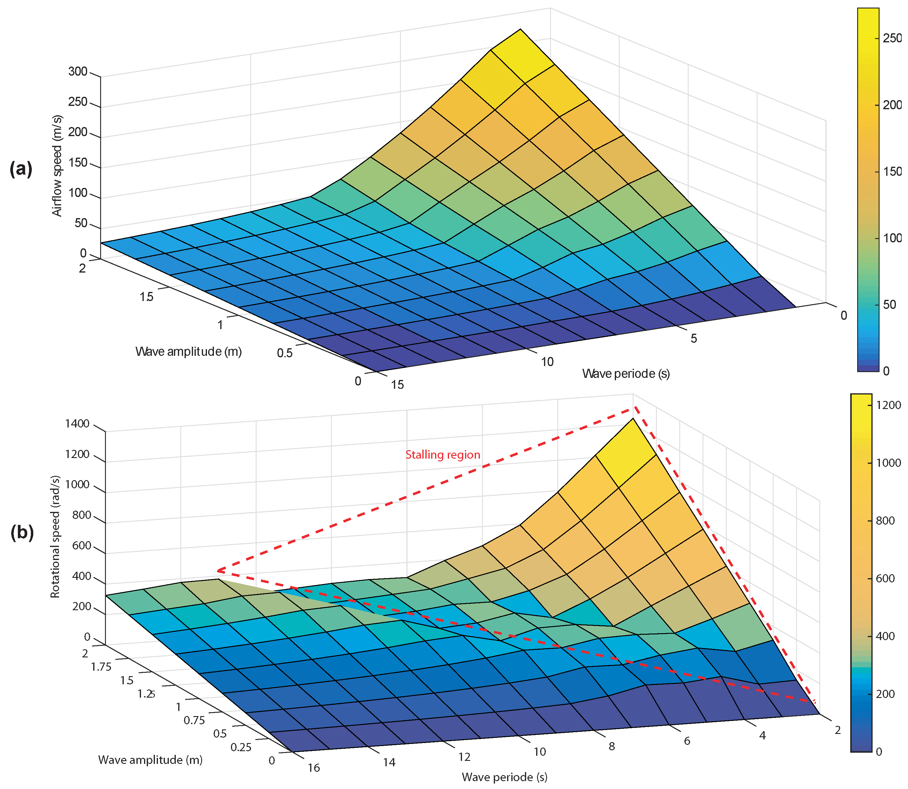
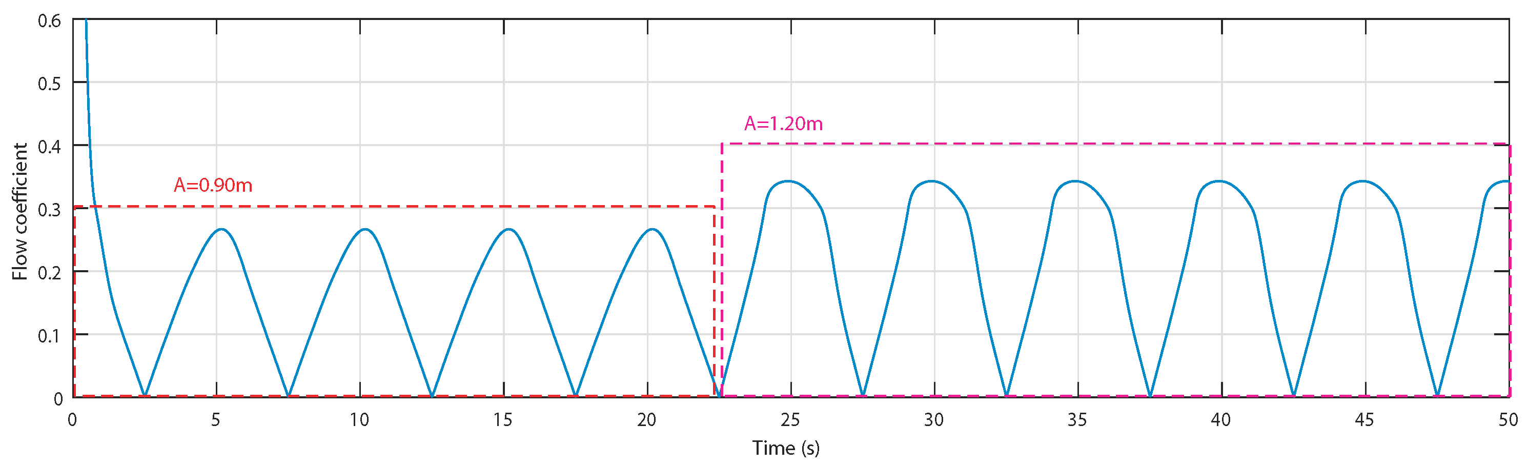
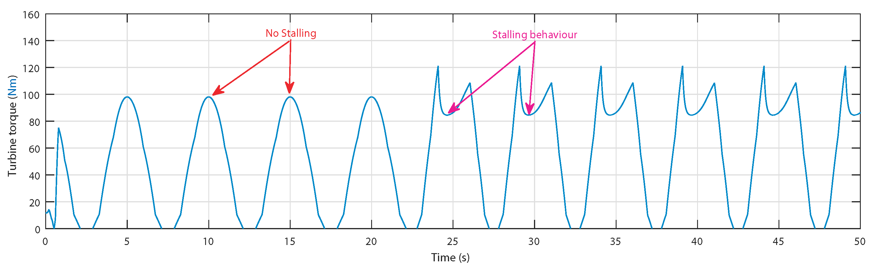
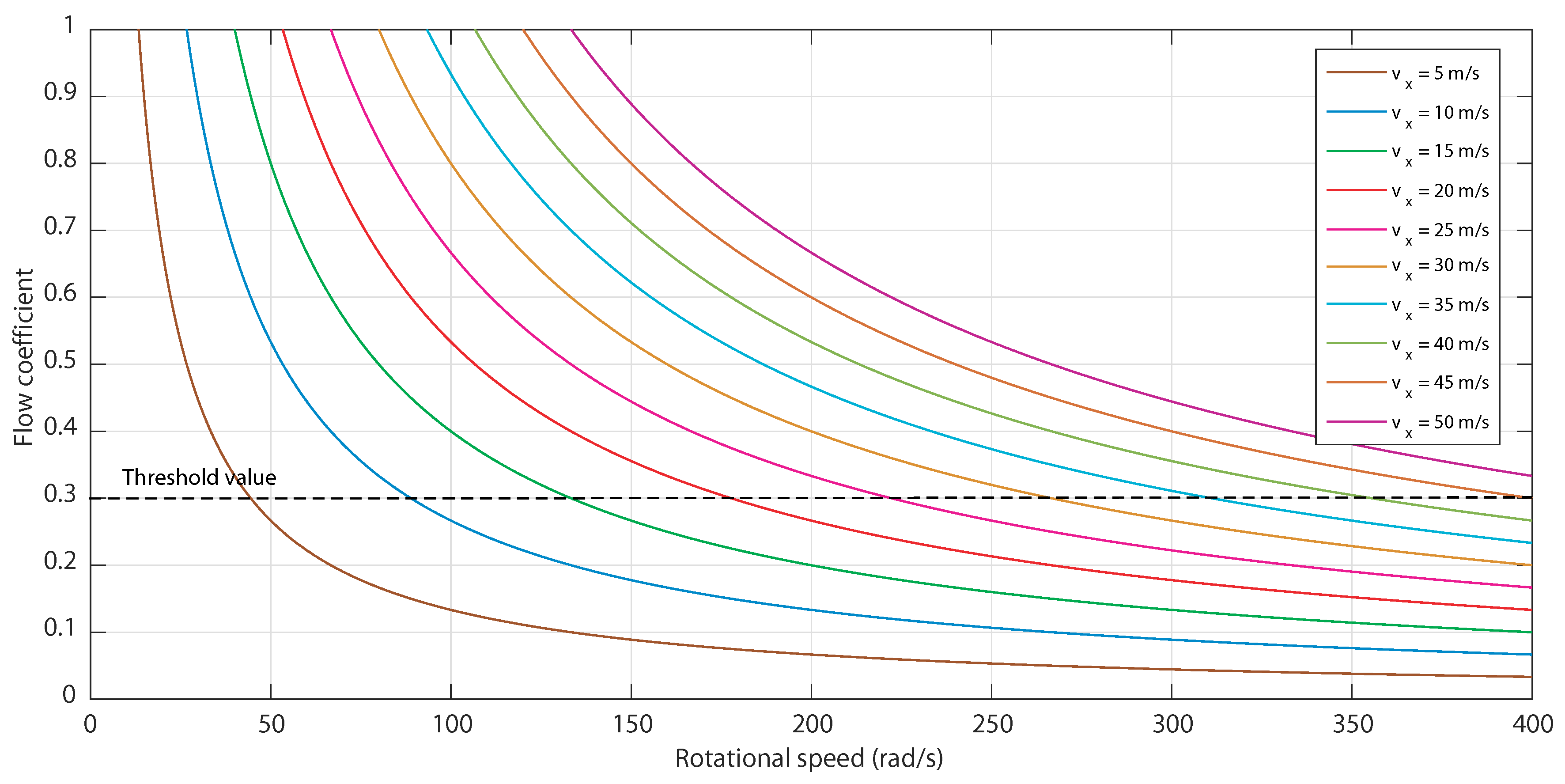
2.6. Stalling Phenomenon

OWC systems consisting of a Wells turbine coupled to DFIG are affected by the stalling behavior when reaching a critical flow rate value v x . The stalling phenomenon occurs when strong waves entering the capture chamber create a strong airflow and the turbo-generator is supposed to keep up with this speed but cannot because the generator is slowing the turbine with its slow dynamics. This is clearly depicted in Figure 4 where the airflow speed v x increases with higher wave amplitudes and sorter wave periods as shown in Figure 4a but the generator stops rotating fast when reaching a certain airflow speed, hence the rotational speed ω r cannot shift fast enough as presented in Figure 4b.
The stalling phenomenon may be interpreted from Figure 3b that shows that when the flow coefficient ϕ exceeds the threshold 0.3 , the torque coefficient C t decreases significantly.
As defined by Equation (10), the flow coefficient ϕ varies with the airflow speed v x . Though Equation (5) describes v x as a function of the wave amplitude and period. In fact, the bigger the wave amplitudes and the smaller the wave periods are, the higher the wave power and the airflow speed are as explicated by Figure 4. Figure 4 also shows that as the airflow speed increases after a certain point the rotational speed cannot keep up with the gradual increase.
The stalling effect is noticed by observing the uncontrolled oscillating-water-column system in two different ocean situations; the first situation is a wave with a 10 s period and 0.9 m wave amplitude from 0 s to 22.5 s and the second situation is a wave with a 10 s period and 1.2 m wave amplitude from 22.5 to 50 s. Figure 5 shows that the first situation offers a flow coefficient less than the threshold value 0.3 however the second situation offers a flow coefficient higher than 0.3.
Because of the flow coefficient of Figure 5, the obtained turbine torques differ at the crest of each wave as illustrated in Figure 6. In fact, no stalling was observed for the first scenario but a significant decline at the crest in the second scenario due to the stalling phenomenon that decreases the average value of the torque.

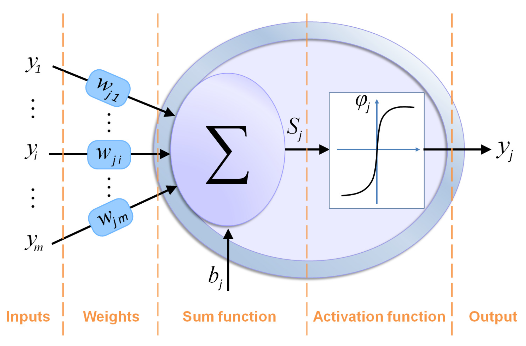
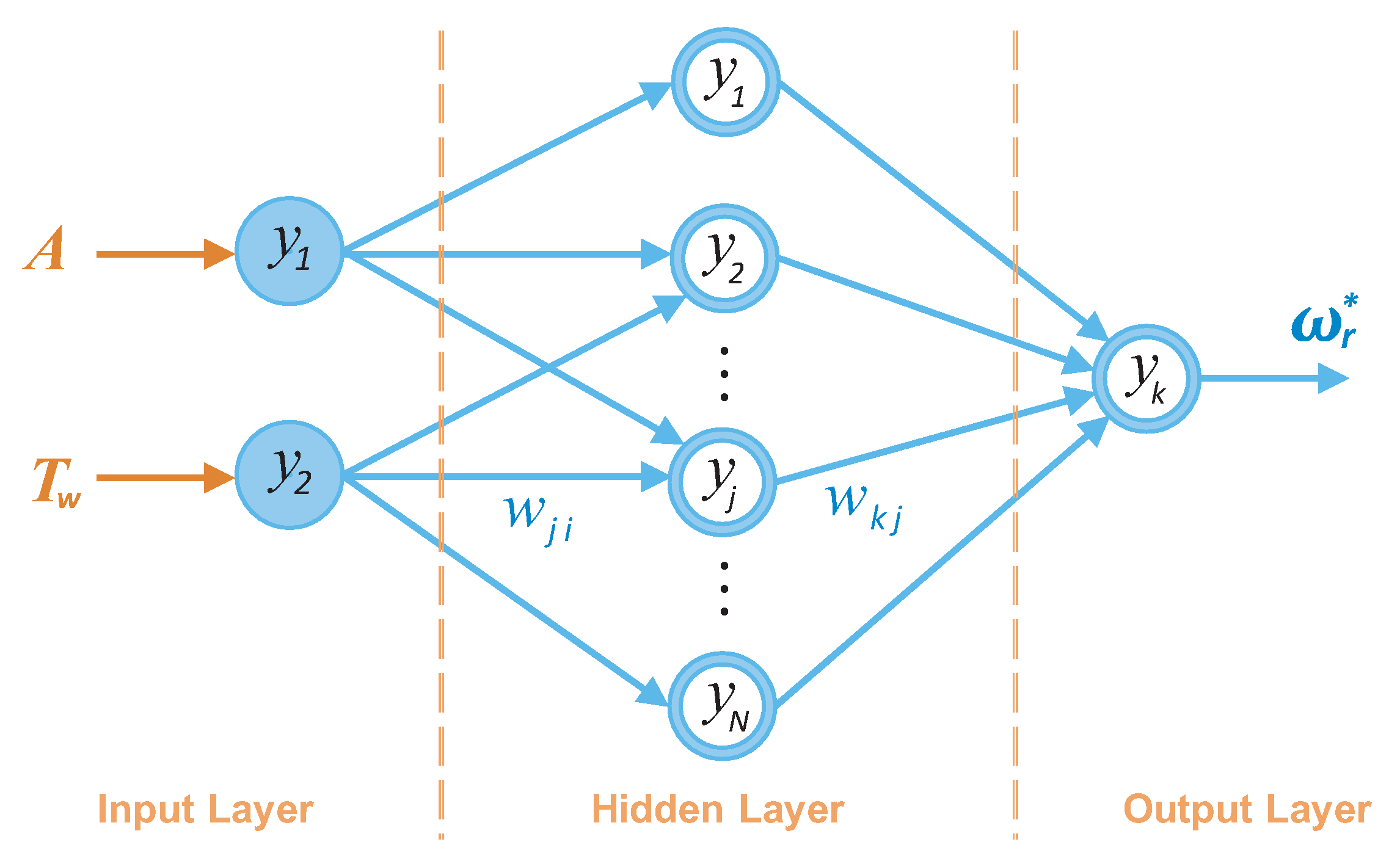
2.7. Artificial Neural Networks

Artificial Neural Networks are rather simple electronic representations based on the biological neural structure of the human brain. ANNs were designed to mimic the behavior of the human neural system without the specific knowledge of the relationships between input data and the target data [33]. This feature made ANNs sought for solving many complex problems where specific knowledge of functions is absent or hard to determine [34,35]. A biological neural network consists of many interconnected neurons whereas ANNs are formed by simple processing units, called artificial neurons.
Artificial Neural Networks are formed of neurons in the input, output and hidden layers that are related with weighted signals ( w j i ). A neuron consists of a bias b j , a sum function S j associated with an activation function φ j as depicted in Figure 7.
The sum function of the jth neuron connected to N neurons from the previous layer is:
S j = j = 1 N ( w j i y i ) + b j
where S j is the sum from the jth neuron from the current layer, b j is the bias, N is the total number of neurons, w j i is the weight of the signal connecting the jth neuron from the current layer with the ith neuron from the previous layer and y i is the input signal from the neuron of the previous layer.
Connected to the activation function the output y j of the jth neuron is defined as:
y j = φ j ( S j ) = φ j i = 1 N ( w j i y i + b j )
The neurons’ activation functions at the input layer are clamped with the input vector but the activation function of the neurons in other layers may be defined as:
φ j ( S j ) = S j ( L i n e a r ) 1 1 + e S j ( S i g m o i d ) e S j e S j e S j + e S j ( H y p e r b o l i c t a n g e n t )
Among the numerous types of ANN, Multi-Layer Perceptron (MLP) is the most common type used as feed-forward ANN. Generally, MLP consists of three layers as depicted in Figure 8. The first layer is the input layer that receives measured data/information. The last layer is called the output layer where the estimated/predicted solution is obtained. The input and output layers are connected by one or more intermediate layers known as the hidden layers. Moreover, MLPs are only connected by feed-forward connections.

3. Materials and Methods

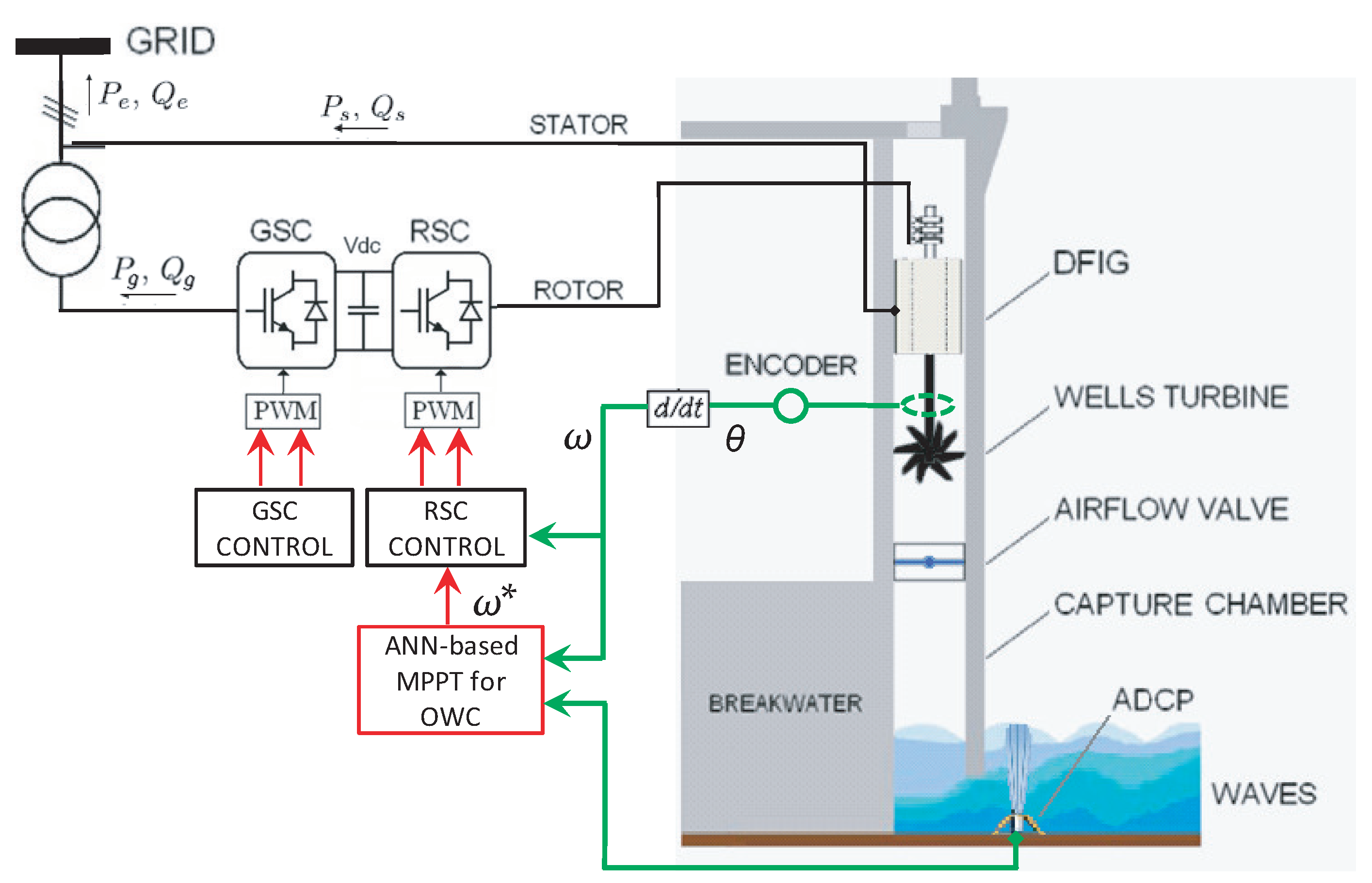
3.1. Proposed ANN-Based Rotational Speed Control

The continuous adjustment of the DFIG’s rotational speed is on way to avoid the stalling phenomenon in the OWC which will increase the extracted power from waves [20,21]. This way, according to Equation (7), the flow coefficient is regulated not to exceed the threshold value 0.3. Therefore, an ANN-based rotational speed control strategy is suggested to adjust the speed ω r of the DFIG in the OWC system via the back-to-back converter and hence maintaining the flow coefficient ϕ below the threshold value. The Artificial Neural Network is going to be trained to be able to recognize waves entering, via measured data with the Acoustic Doppler Current Profiler (ADCP). The scheme of the suggested ANN rotational speed control strategy is explained by Figure 9.
Each side of the BTB converter controls a different aspect of the plant. The GSC adjusts the DC-link voltage and reactive power, whereas the RSC adjusts the active power and rotational speed.

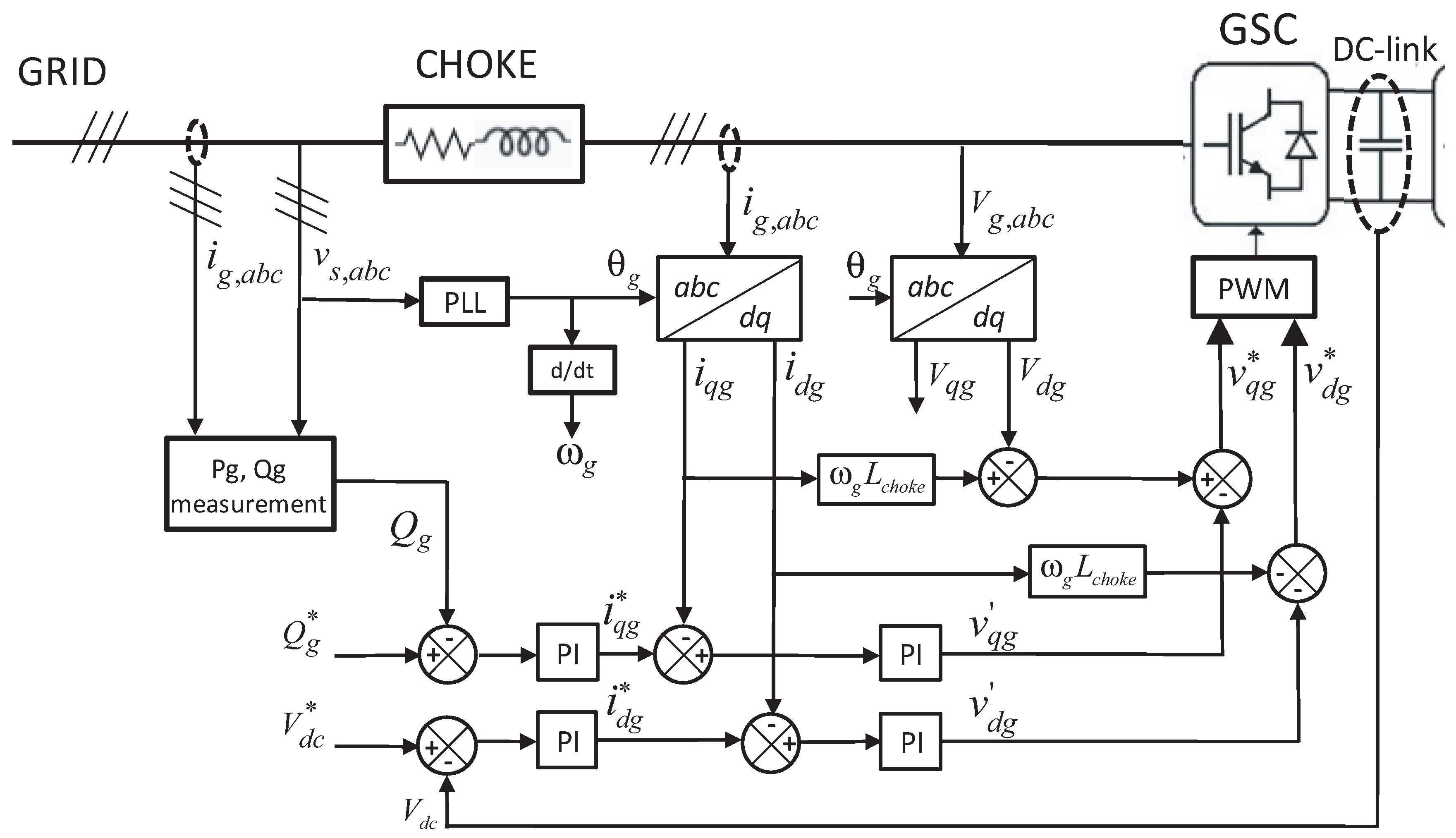
3.1.1. Grid-Side Converter Control

The vector control based on Voltage Oriented Control has been adopted for the GSC therefore the d-axis is aligned with the grid voltage vector [29]. Hence v d g = v g and v q g = 0. Thus, the grid’s active and reactive powers may be written as:
P g = 3 2 v d g i d g Q g = 3 2 v d g i q g
Thanks to the Voltage Oriented Control the equations of voltages across the grid are:
v d g = R g i d g + L g d i d g d t ω g L g i q g Δ v d g + u d g 0 = R g i q g + L g d i q g d t + ω g L g i d g Δ v q g + u q g
where Δ v d g and Δ v q g are feed-forward compensation terms which are added back to the control signals.
Figure 10 shows the control scheme used to regulate the DC-link voltage and reactive power. The control scheme consists of two rows of two PI controllers in series.
The outer loops regulate the grid currents and generate the reference currents i d g * and i q g * using PI controllers. The PI controllers receive as reference inputs both the grid’s reactive power Q g * , frequently set to zero, and the reference DC voltage V D C * = 800 V. The obtained i d g * and i q g * currents are the reference inputs of the inner loops’ PI controllers. The inner loops generate reference voltages v d g and v q g which are compensated to get the required v d g * and v q g * for the Pulse Width Modulation.

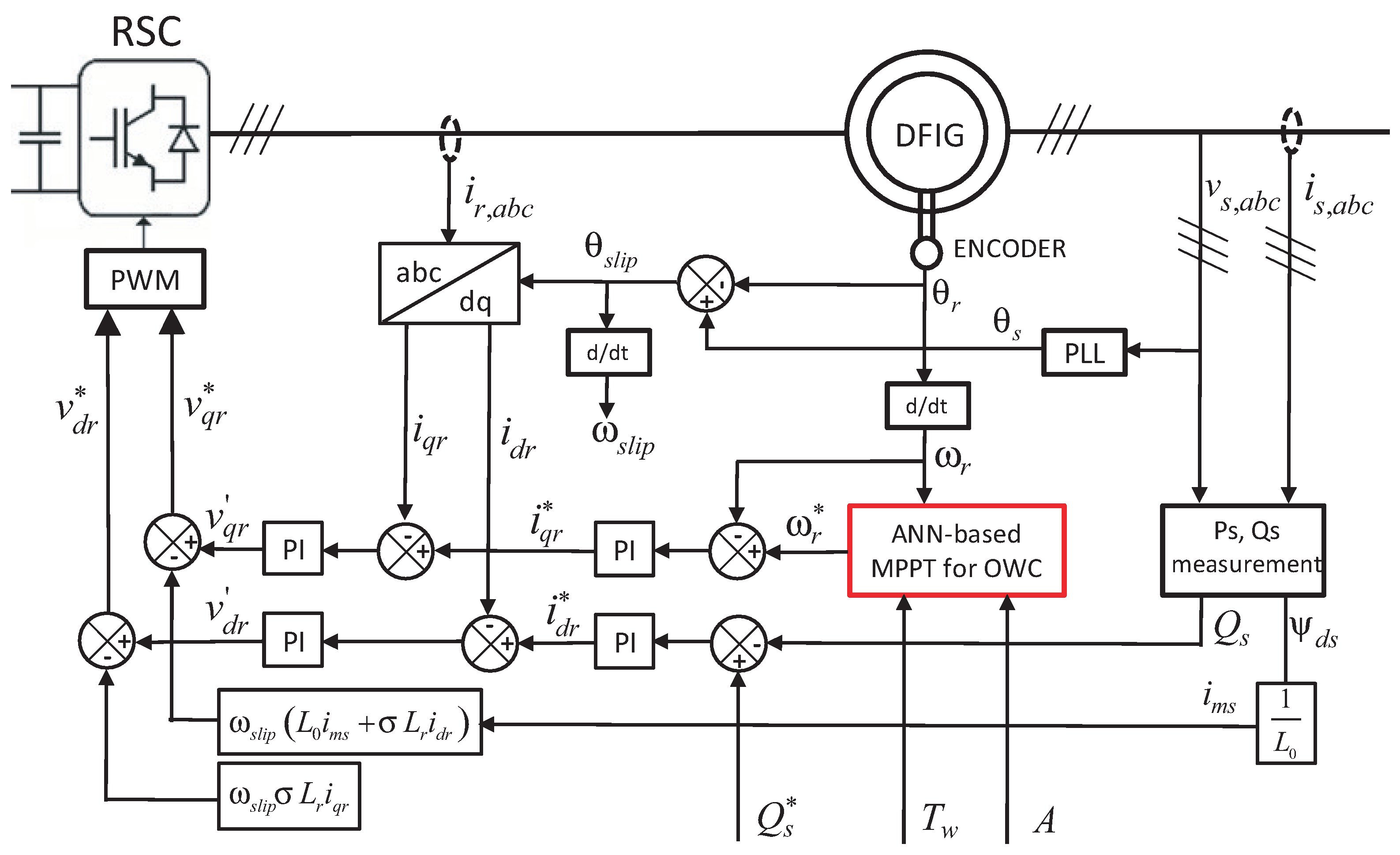
3.1.2. Rotor-Side ANN Rotational Speed Control

For the rotor-side converter the doubly fed induction generator is controlled by the Stator-Flux Orientation to align the d-axis with the stator-flux vector [27]. Hence ψ d s = ψ s and ψ q s = 0. Thus, the stator currents and stator voltages may be written as:
i d s = 1 L s ψ s L m i d r i q s = L m L s i q r v d s = ψ s L s R s L m L s R s i d r v q s = ω s ψ s L m L s R s i q r
Using (30), the stator active and reactive powers also may be written as:
P s = 3 2 ψ s L s R s L s ψ s + L m ω s i q r Q s = 3 2 ψ s L s ω s ψ s + L m ω s i d r
Looking into (31), it indicates that the direct rotor-current i d r is controlled to regulate the reactive power whereas the quadrature rotor-current i q r is controlled to regulate the active power.
Thanks to the Stator-Flux Orientation the rotor voltages can be written as:
v d r = R r i d r + L r d i d r d t ω s l i p σ L r i q r Δ v d r v q r = R r i q r + L r d i q r d t + ω s l i p σ L r i d r + ω r L 0 i m s Δ v q r
where Δ v d r and Δ v q r are feed-forward compensation terms which are added back to the control signals.
The control scheme of rotor-side converter is illustrated in Figure 11 which uses two PI controllers to regulate the rotor currents i d r and i q r . Another two PI controllers, in cascade to the outer loops PI controllers, are used to regulate the desired rotor voltages.
As with the grid-side converter control, the outer loops produce i d r * and i q r * by using as reference inputs the stator reactive power Q s * and the rotational speed ω r * . Q s * is set to zero whereas ω r * is provided by an ANN-based MPPT for OWC. The reference voltages v d r and v q r are generated by the inner loops which are compensated to obtain v d r * and v q r * .

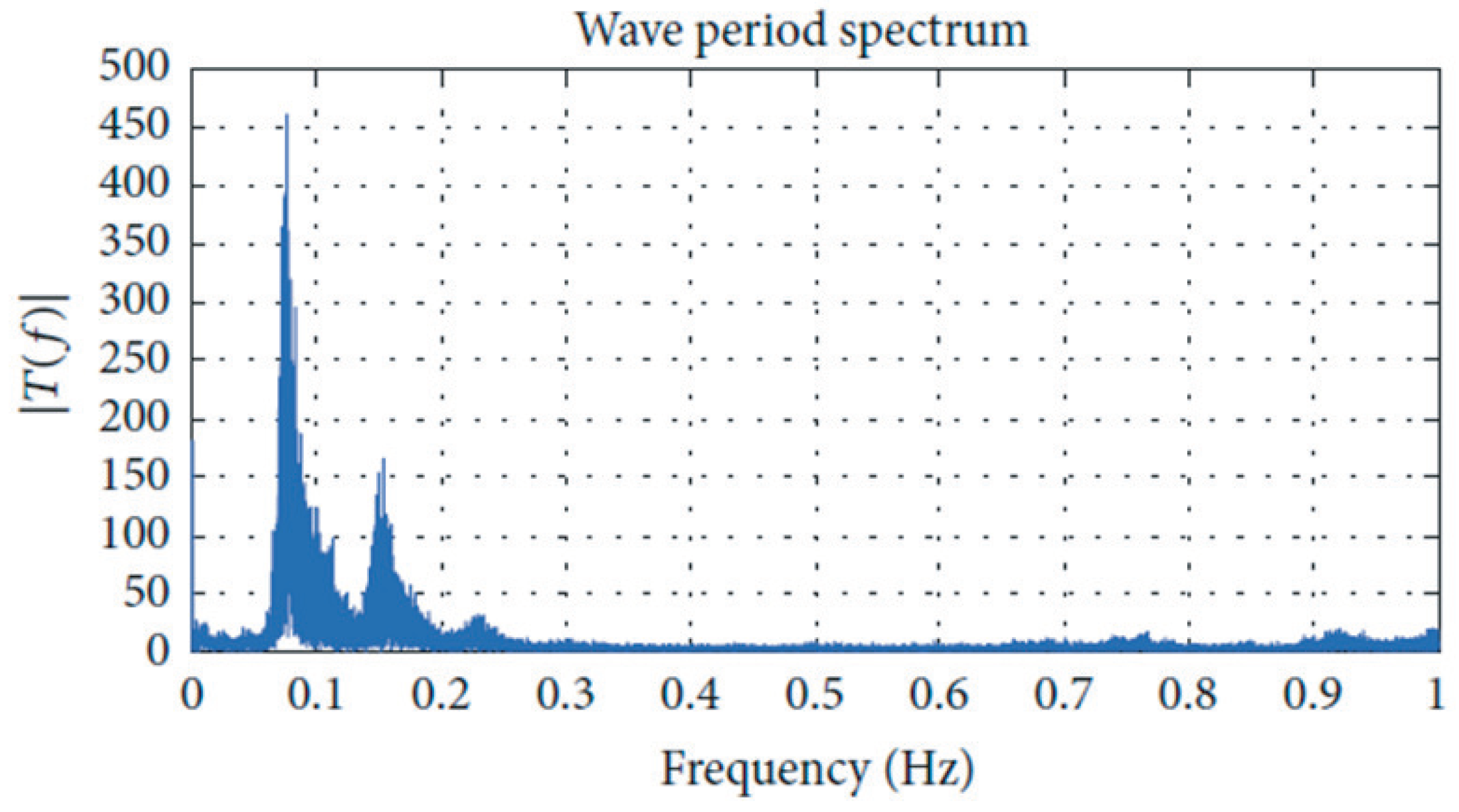
3.2. Gathering Wave Data

The artificial neural network has been trained to identify waves entering the OWC using measured data. The data were collected by AZTI-Tecnalia at the breakwater of Mutriku in the northern coast of Spain using an Acoustic Doppler Current Profiler (ADCP) depicted in Figure 12.
ADCP is a hydro-acoustic measurement tool for measuring water current speeds. This device works with the Doppler effect of sound waves returned from particles. ADCPs can send and receive sound signals using a piezoelectric transducer. The distance is estimated based on the time sound waves travel back. The frequency shift of the echo is proportional to the water velocity within the acoustic path. Measuring 3D speed needs at least three beams [36,37].
Recently further features were included to ADCPs to measure wave and turbulence data. The specific ADCP instrument for wave characteristic measurements is called the Acoustic Wave and Current (AWAC) profiler. It offers the possibility of measuring the wave’s height and direction [38,39]. The AWAC system uses four transducers to transmit four beams; one middle transducer points vertically upward, and three transducers positioned symmetrically at 120 degrees from each other and are angled 25 degrees from the vertical axis [40,41].
The device installed in Mutriku is of Workhorse 600 kHz from Teledyne RDI and it is mounted upside down at the seafloor 1 m in front of the openings of the OWC’s capture chamber. This distance is 5 times smaller than the wavelength λ (see Figure 1) which allows the registered wave trains to enter the chambers without the risk of changing. The considered data in this paper are from 12 May 2014 where measurements of the first 20 min were recorded every 2 h and with a sampling period of 0.5 s. The data were gathered and treated by AZTI-Tecnalia and a spectral analysis has been performed. The wave spectrum of the site of Mutriku is illustrated in Figure 13.

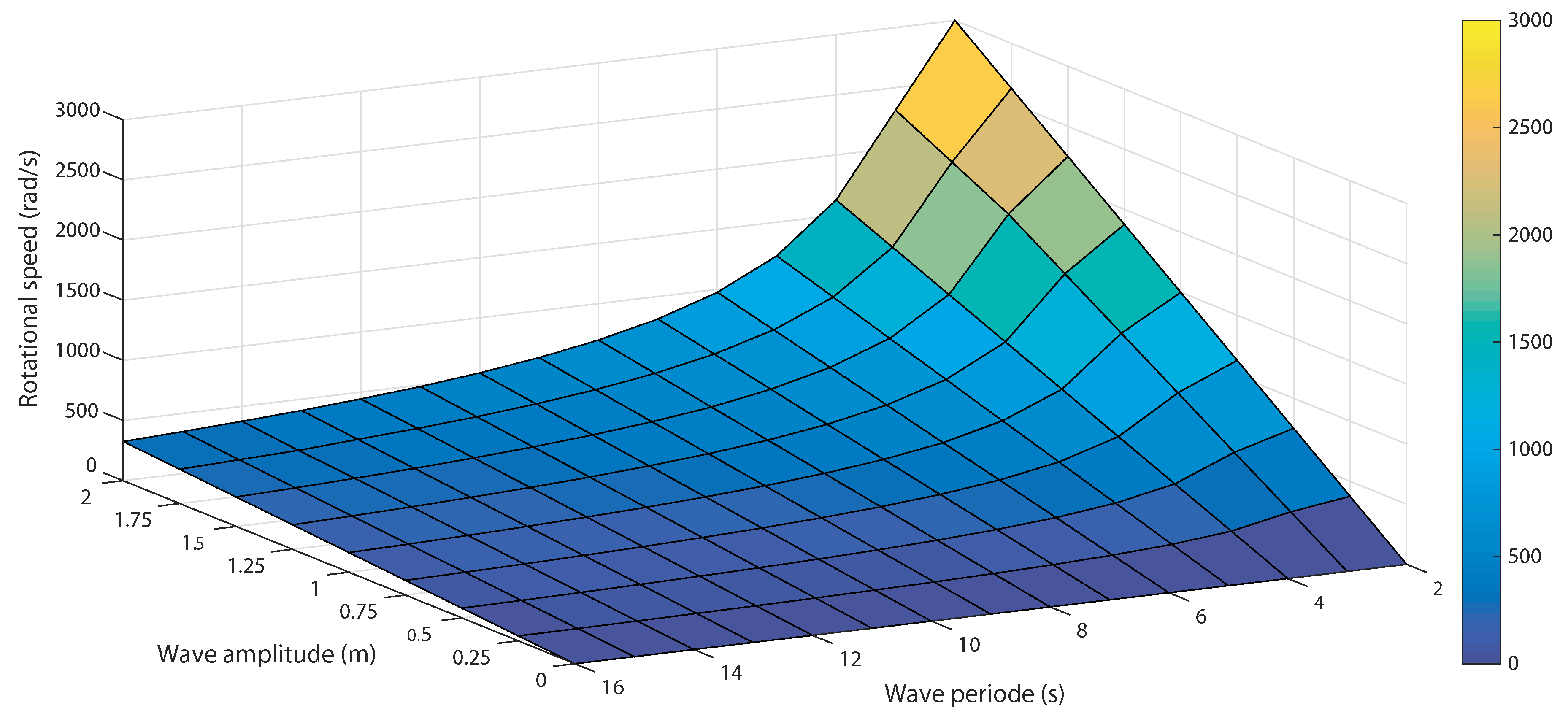
3.3. ANN-Based MPPT Design

The trained ANN must generate reference rotational speed ω r * for the outer loop of the RSC control scheme has been developed for a Wells turbine-based oscillating water column. The developed control considers the characteristic curve of Figure 3b with the intention of avoiding the stalling effect. Therefore, the MPPT will generate the optimum ω r * according to the incident wave. Thus, many simulations have been carried out to monitor the flow coefficient for different wave amplitudes and periods yielding the plots of Figure 14 from which the optimum ω r * may be obtained.
For the same incoming airflow speed from the same wave amplitudes and periods the torque obtained against the rotational speed is presented in Figure 15.
It is indicated in Figure 14 and Figure 15 that the extractable torque is high when the flow coefficient is below the threshold value 0.3 and is highest when it reaches 0.3 which corresponds to optimal ω r * . This approves the aforementioned power constraint triggered by the stalling phenomenon. Therefore, many simulations have been performed to obtain the minimum rotational speed for corresponding wave amplitudes and periods. Hence, input and output data sets were assembled to train the ANN to provide the required rotational speed output. The desired rotational speed reference against the wave amplitude and period is illustrated in Figure 16.
The optimum rotational speed in Figure 16 increases as the incoming airflow provided by the strong waves increases unlike the rotational speed shown in Figure 4b which slows down after a certain critical point.
The model of a designed ANN is determined by three features; first, the structure of the network, second, the neuron characteristics, and third, the training algorithm.
The structure of the developed ANN in this work is a Multi-Layer Perceptron (MLP) meaning all links are feed-forward connections. The ANN is formed of a 2-node input layer; one node for the wave amplitude A and the second node for the wave period T w , a hidden layer formed of variable number of hidden nodes and layers, and an output layer that has only one node for the solution which is the reference rotational speed ω r * as explained in Figure 8. The neurons used in the hidden layers are characterized by hyperbolic tangent activation function whereas in the output layer the linear activation function was used.
The developed ANN has been trained using the Levenberg–Marquardt Algorithm (LMA) which combines the gradient descent and Gauss-Newton methods [42]. The training algorithm allows the update of the weights connecting the neurons in order to improve the outcome. This is achieved through the update expression defined as follows:
w j i ( p + 1 ) = w j i ( p ) + Δ w j i ( p )
where w j i ( p + 1 ) is the new calculated weight, w j i ( p ) is the current weight and Δ w j i ( p ) is the weight correction obtained by the chosen training algorithm.
Selecting the needed hidden layers and neurons in a complex system is a difficult task thus forward approach-based trial-and-error rule procedure is adopted [43]. This approach starts by a small number of hidden layers/neurons and increases their number. Then every new ANN structure is trained and tested. This process is repeated until the train and test results are improved.

3.4. ANN Training Process

For the training of the network the Levenberg–Marquardt Algorithm (LMA) has been used as a learning technique [42]. LMA is based on Newton’s technique that was developed to minimize functions that are sums of squares of nonlinear functions [44]. The algorithm is intended to update the ANN weights to minimize the performance index by [45]:
Δ W = 2 F ( W ) + μ I 1 F ( W )
where W is weights vector, F ( · ) is the performance index, F ( · ) is the gradient, 2 F ( · ) the Hessian matrix, μ is the learning rate and I is an identity matrix.
The performance index may be described by:
F ( W ) = j = 1 N E j 2 ( W ) = E T ( W ) . E ( W )
with E ( · ) is the error between the network’s output and the desired output.
The performance index’s gradient can be given by:
F ( W ) = 2 J T ( W ) . E ( W )
where J ( W ) is the Jacobian matrix defined as [46]:
J ( W ) = E 1 ( W ) W 1 E 1 ( W ) W 2 E 1 ( W ) W n E 2 ( W ) W 1 E 2 ( W ) W 2 E 2 ( W ) W n E N ( W ) W 1 E N ( W ) W 2 E N ( W ) W n
with n is the number of training patterns.
Consequently, the Hessian matrix can be described by:
2 F ( W ) = 2 J T ( W ) . J ( W ) + 2 j = 1 N E j ( W ) . 2 E j ( W )
The pseudocode Algorithm 1 is given to detail the steps of the Levenberg–Marquardt Algorithm.
Algorithm 1: Levenberg–Marquardt Algorithm (LMA)
1. Initialize training parameters: μ , μ m a x , β , E m i n , E p o c h , E p o c h m a x .
2. Initialize weights vector W p with small random numbers.
3. Calculate error E p and performance index F using Equation (35).
4. Calculate Jacobian matrix J and Hessian matrix H using Equations (37) and (38).
5. Calculate weight corrections Δ W using Equation (34).
6. Update weights W p + 1 using Equation (33).
7. Using new weights calculate and evaluate new error E p + 1 :
  (i) if E p + 1 > E p then • Reset weights to previous values W p = W p ,
            • Increase learning rate by a factor β : μ = μ . β ,
            • Return to step 4.
  (ii) if E p + 1 E p then • Save new weights as current values W p = W p + 1 ,
            • Decrease learning rate by a factor β : μ = μ / β ,
            • Return to step 3.
8. Continue training until one of the following termination conditions is reached:
   ( E p o c h > E p o c h m a x ) or ( μ > μ m a x ) or ( E p E m i n )
The training and validation of all tested ANN structures was performed using MATLAB R2015a while using 3.2 GHz Intel Core i7-8700 Six-Core processor and Integrated Intel UHD Graphics 630.

3.5. ANN Model Selection

The Mean Squared Error (MSE) has been chosen in this work as a selection criterion for the ANN model to be used in the proposed airflow control. The MSE is one of the indicators often used in prediction problems [47]. The best ANN structure is selected by choosing the smallest MSE obtained during the training process.
The Mean Squared Error was computed in every case using the following expression:
M S E = 1 n i = 1 n ( Y i Y ^ i )
where n is the total observations, Y i is the target output being the desired rotational speed reference and Y ^ i is the predicted output by the ANN.

4. Results and Discussion

This section of the paper presents the tests performed to assess the efficiency of the developed ANN-based rotational speed control. A complete wave-to-wire model on MATLAB/Simulink of the oscillating-water-column system has been implemented for performance evaluation of the suggested control and a comparison with the uncontrolled case has been carried out.
The implemented OWC model has been configured using the parameters obtained from real measurements at the NEREIDA wave power plant. These parameters were provided by the Basque Energy Agency (EVE) and are indicated in Table 1.

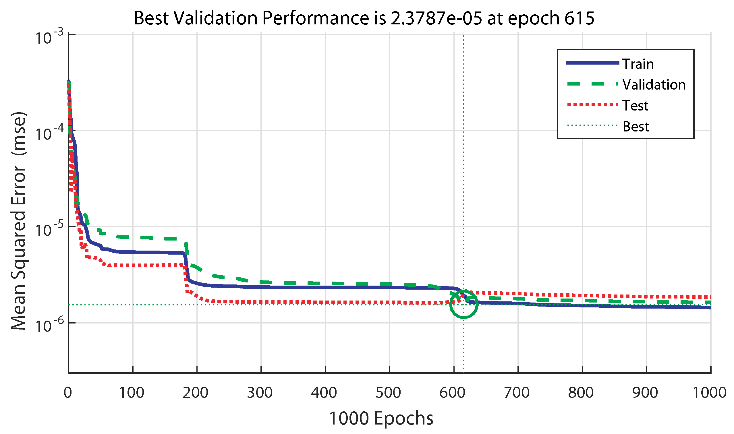
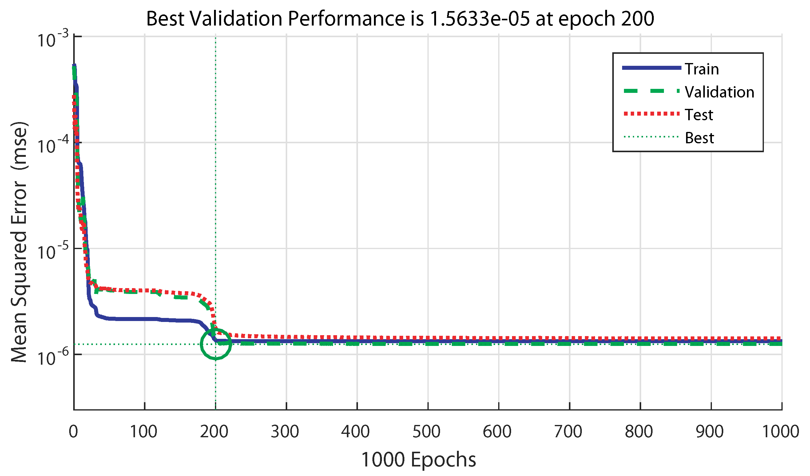
4.1. ANN Training Performance

With the forward approach-based trial-and-error rule method, numerous structures with different hidden layers and neurons have been tested with our problem. For the training process, the data were divided into 40% for the learning stage, 30% for the testing stage and 30% for the validation stage.
The results of calculations for determining the ANN model are detailed in Table 2. The results of training show that the best neural model that has been calculated is the MLP 2 × 4 × 8 × 1 with 2 neurons on the input layer (for the wave amplitude and period), 4 neurons on the first hidden layer, 8 neurons on the second hidden layer and 1 neuron on the output layer (for the rotational speed reference). The second best MLP is 2 × 4 × 4 × 1 with 2 neurons on the input layer, 4 neurons on the first hidden layer, 4 neurons on the second hidden layer and 1 neuron on the output layer. These two nets have the best learning, testing and validation qualities moreover, their validation quality is not lower than that of the learning and testing qualities.
During the simulations, the study case takes into consideration the number of epochs and the smallest MSE. Table 3 shows the validation results obtained of training different network structures applied to the problem of wave characteristics recognition.
Results of Table 3 indicate that using a network with a single hidden layer provides less accurate results due to the nonlinearity and complexity of the problem. On the other hand, multiple hidden layer networks provide better results. However, when increasing the number of neurons in the hidden layers and the number of epochs the obtained MSE is worsened. This is due to the overlearning effect. More analysis has been performed on the curves of the training performance of the multiple hidden layer networks with the best MSE labeled as ANN1 and ANN2 for adequate structure selection.
The training process history of ANN1 (2 × 4 × 8 × 1) is given by Figure 17 while the one of ANN2 (2 × 8 × 4 × 1) is given by Figure 18. Both figures indicate that for ANN1 the training process took more epochs to converge to a minimum MSE of 2.3787 × 10 5 in 615 epochs however with ANN2 it converged to a smaller MSE of 1.5633 × 10 5 in fewer epochs at 200.
Finally, ANN2’s structure has been chosen as ANN rotational speed reference generator to be used in the developed rotational speed control strategy with real measured data.

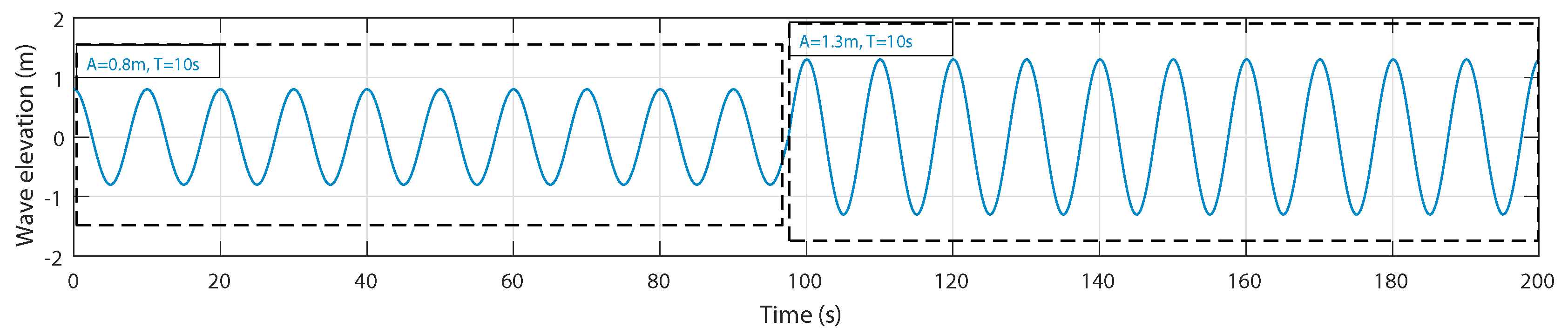
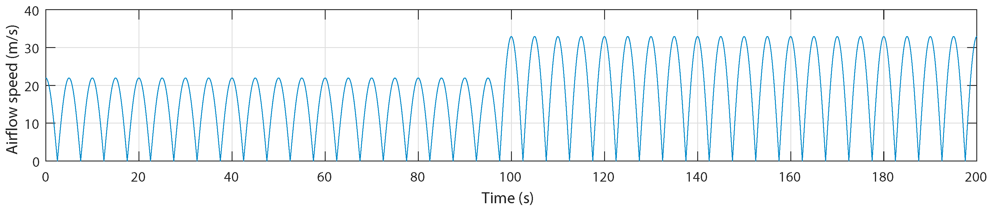
4.2. Control Assessment with Regular Waves

To assess the power generation improvement offered by the proposed ANN-based rotational speed control strategy, a comparative study using ANN1 and ANN2 with two representative sea conditions from the coast of Mutriku were considered from the wave spectrum of Figure 13.
The wave’s input features consist of a water depth h = 5 m and a wave period T w = 10 s. The first wave condition has an amplitude of A = 0.8 m from 0 s to 97.5 s while the second wave condition has an amplitude of A = 1.3 m from 97.5 s to 200 s as presented in Figure 19.
Figure 20 shows the airflow speed for both waves in the uncontrolled case. With the second wave the airflow speed is stronger which will provoke the stalling behavior.
To prevent the stalling phenomenon, the proposed ANN rotational speed control increases the speed when the critical values are reached as shown in Figure 21. This successfully increases the speed in terms of average value from 264.2 rad/s to 272.6 rad/s using ANN1 and 274.1 rad/s using ANN2.
Figure 22 shows the flow coefficients which, in the first wave, did not exceed the threshold value 0.3 in the uncontrolled so no control action was required in the controlled case. However, in the second wave, the flow coefficient exceeds the threshold value hence the increase of the rotational speed helped adjusting it.
Figure 23 presents the obtained torques and it is indicated that in the case of the second wave condition the torque in the uncontrolled OWC has decreases significantly at every crest reducing the torque’s average value to 61.16 Nm. On the other hand, while using the ANN rotational speed control the torque has been held at the highest speed which offered a higher average value of 63.02 Nm using ANN1 and 66.22 Nm using ANN2.
Figure 24 presents the produced power which is negative because it is absorbed by the grid. The produced power did not suffer a power drop at the crests of the second wave condition. As a result, the average value of the produced power has increased to −16.51 kW using ANN1 and −17.39 kW using ANN2 compared to −15.52 kW in the uncontrolled case. From these results the total power increase obtained from using the ANN rotational speed control for only 50 s is 19.36 kW corresponding to 2.53% for one OWC.

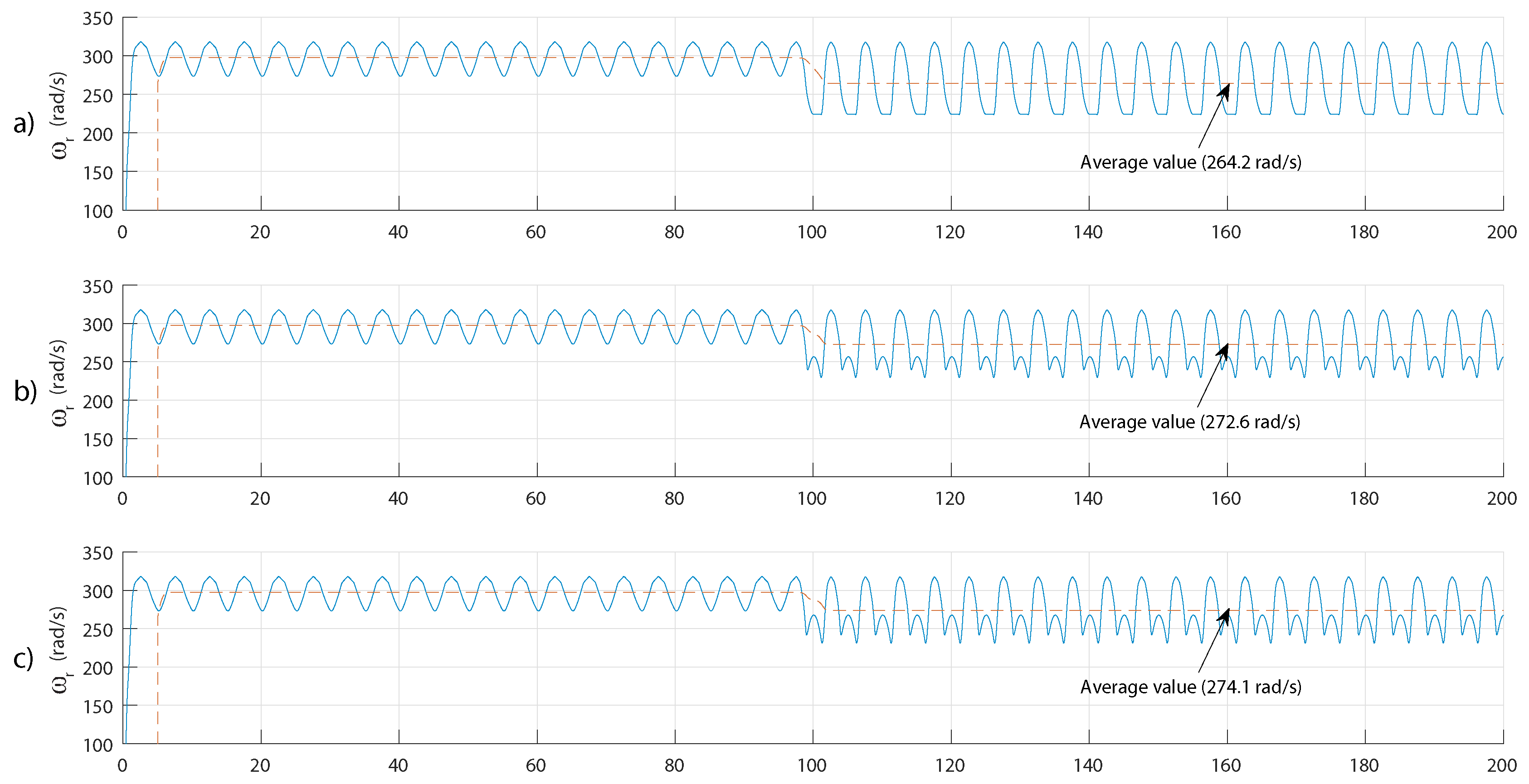
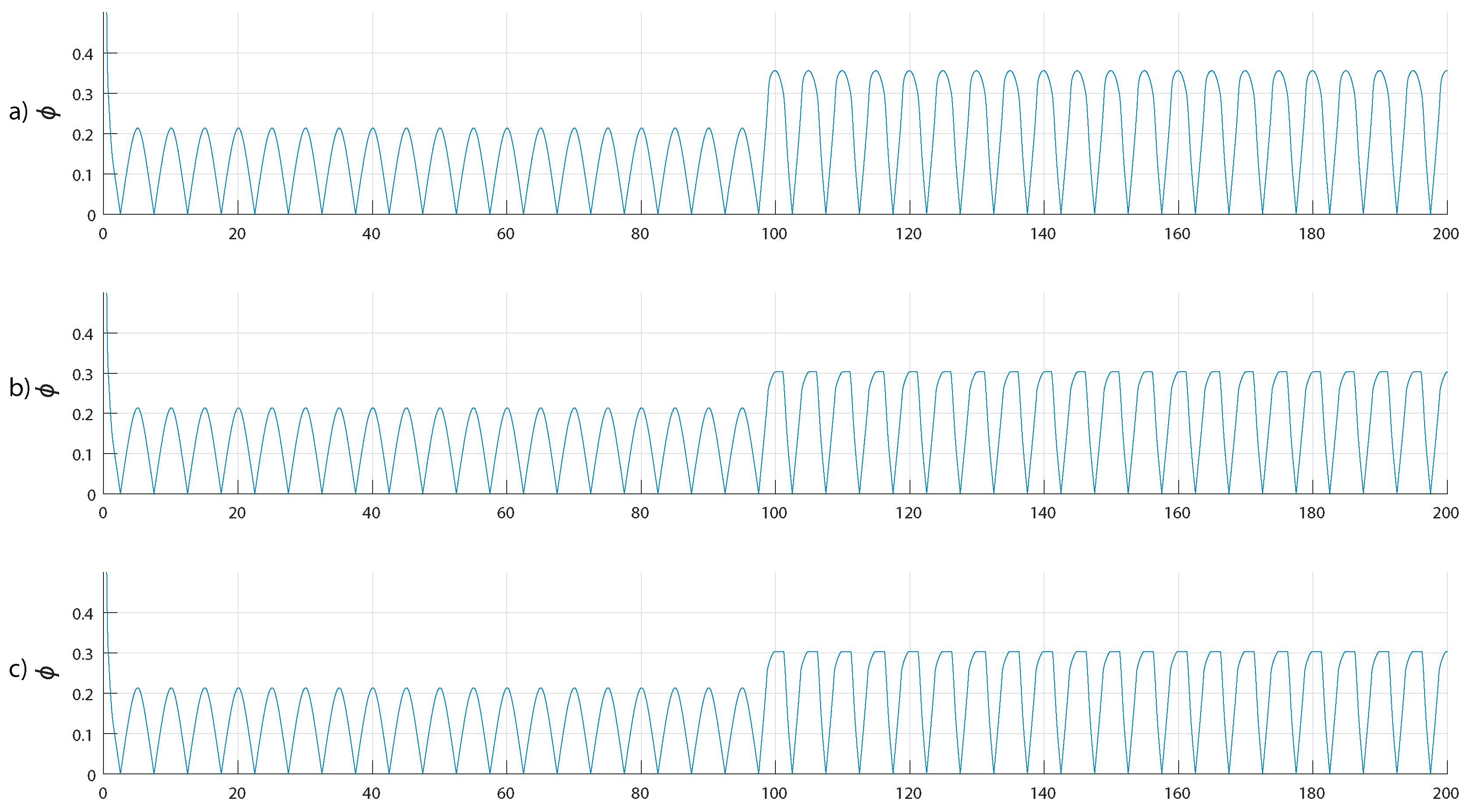
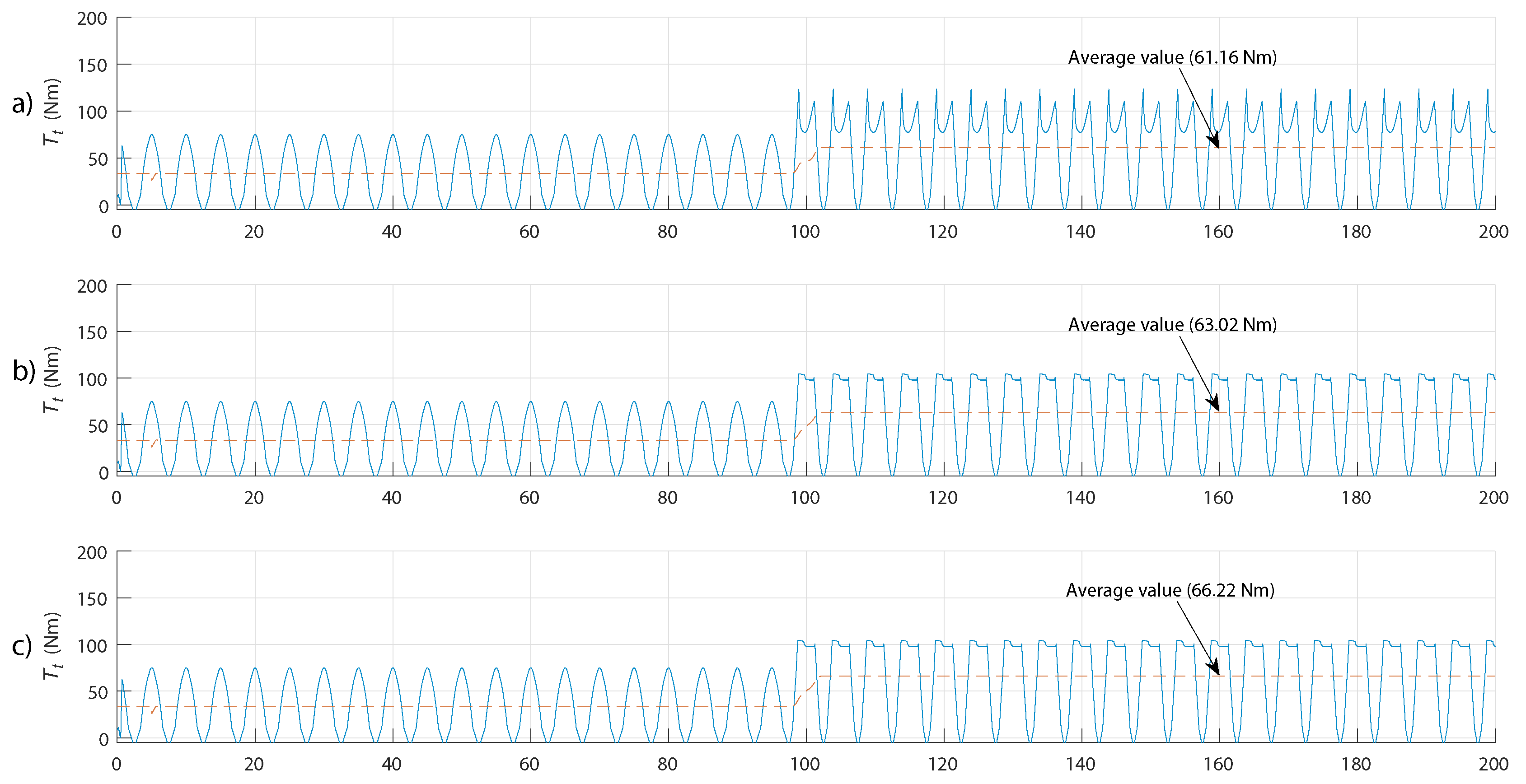
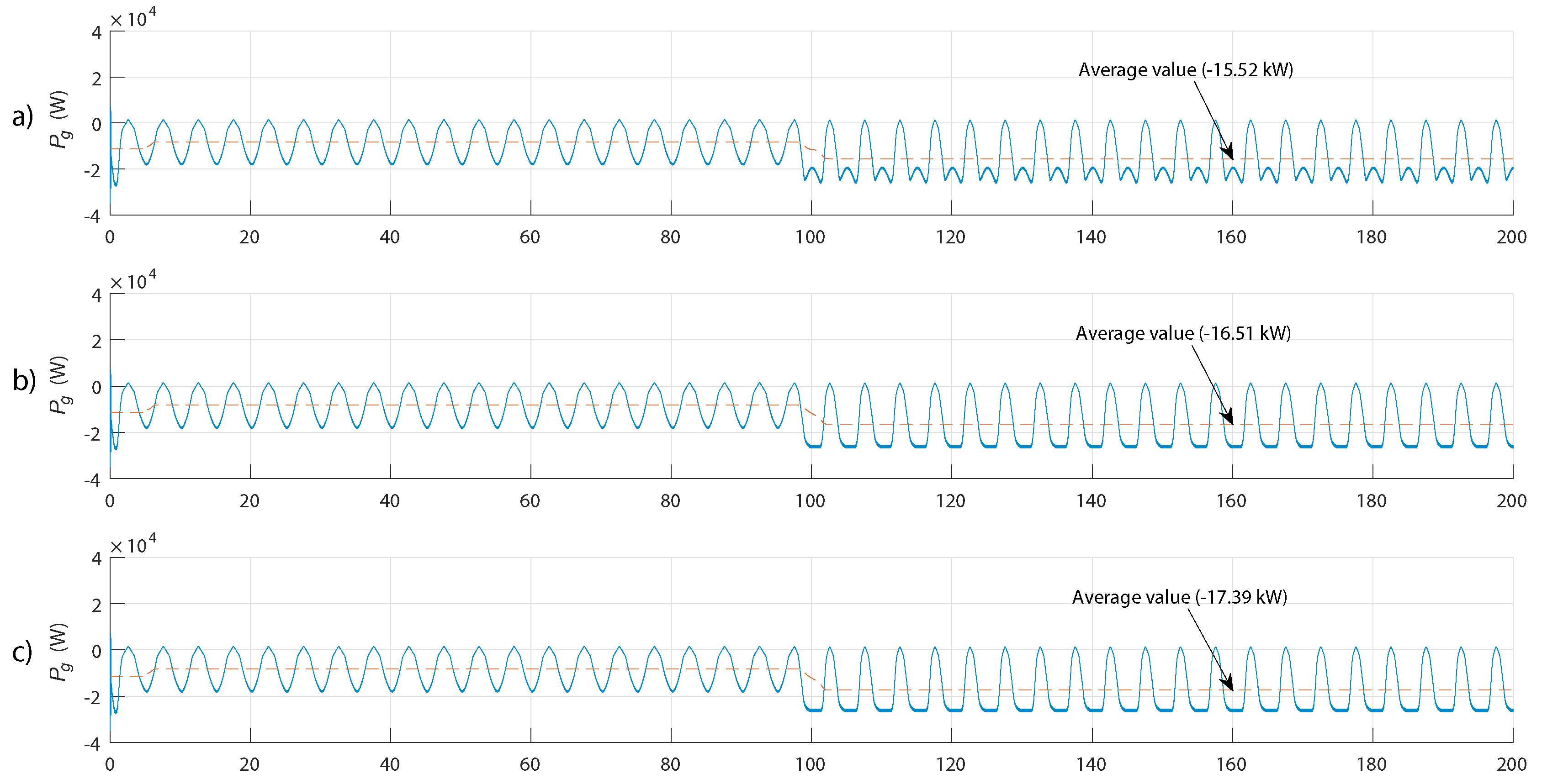
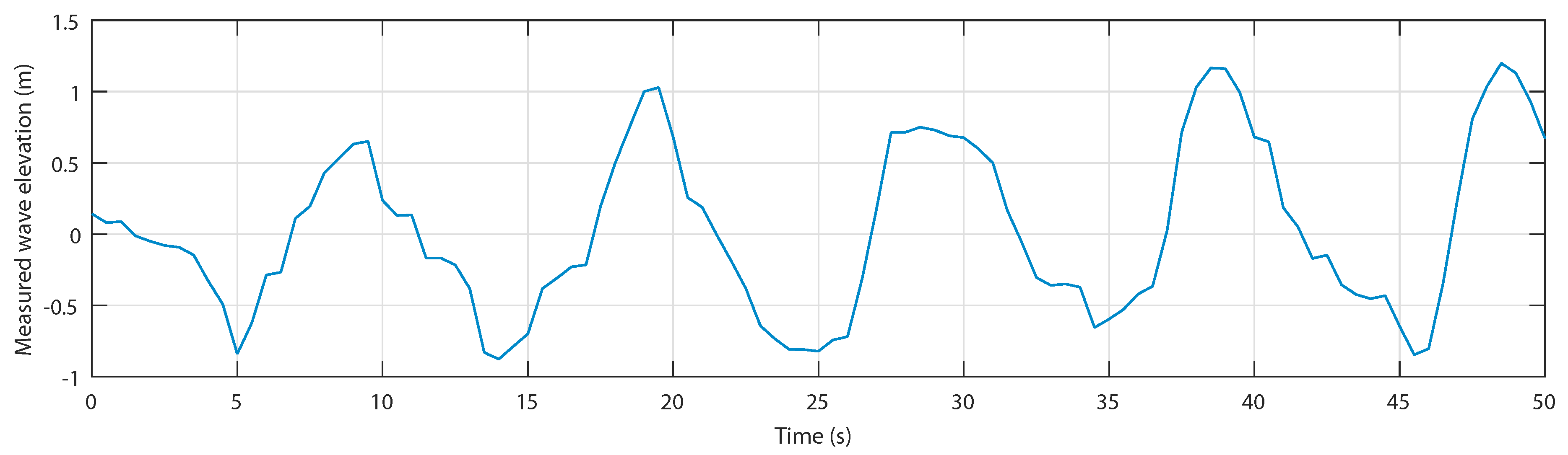
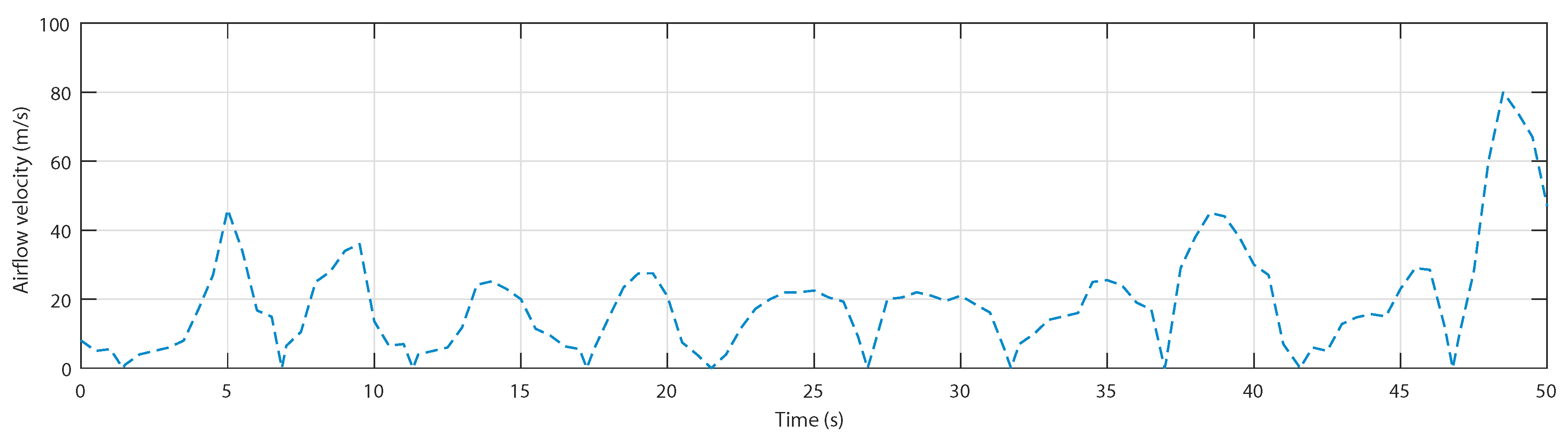
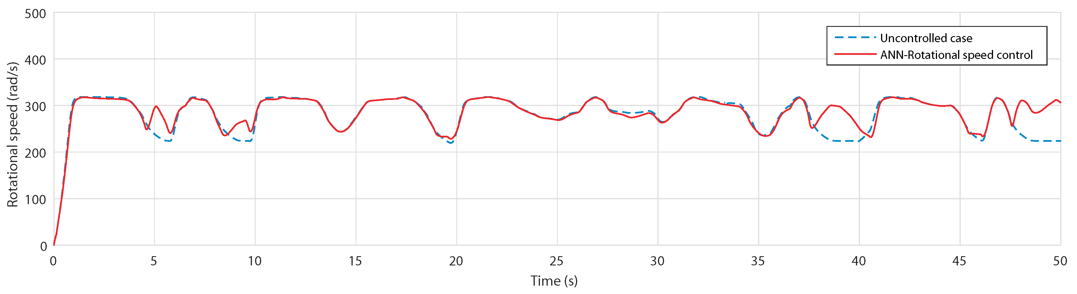
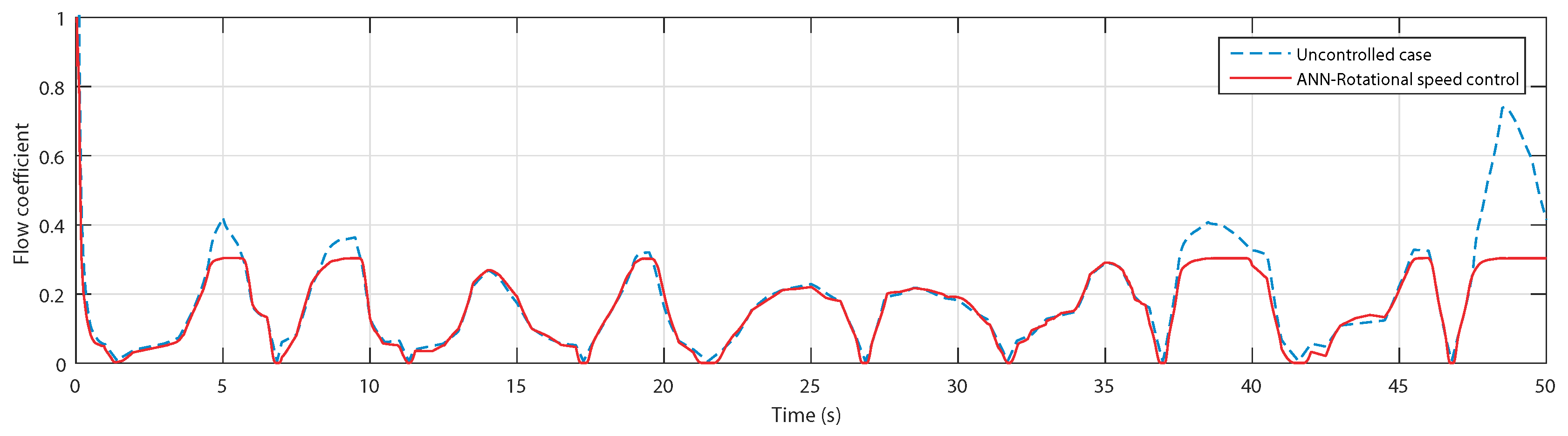
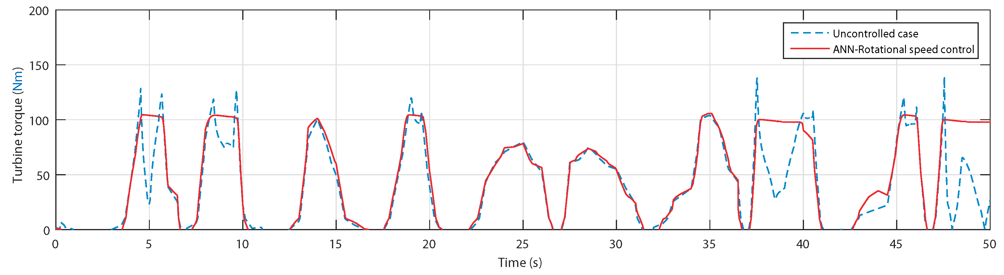
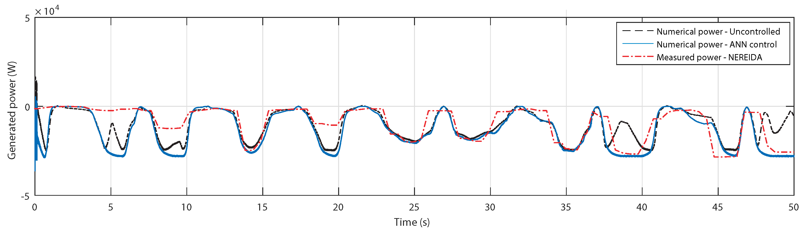
4.3. Control Assessment with Real Measured Wave Data

To further validate the effectiveness of the proposed control, real wave surface elevation data has been considered. Figure 25 illustrates the wave data that were gathered by an ADCP on 12 May 2014, at 00:00:00 AM at Mutriku. This input wave data will allow us to investigate the developed ANN-based rotational speed control strategy with different wave amplitudes and periods in realistic conditions.
The airflow speed is shown in Figure 26 with high airflow at the crest of the waves namely at 5 s, 8 s, 38 s and 48 s.
Figure 27 shows the rotational speed in the uncontrolled case and with the ANN rotational speed control. To keep up with the airflow speed and evade the stalling phenomenon, the ANN rotational speed control increases the speed.
As a result, the flow coefficients presented in Figure 28 have surpassed the threshold value at 5 s, 8 s, 38 s and 48 s in the uncontrolled case. However, in the controlled OWC the coefficient has been regulated.
The produced torques presented in Figure 29 show that the torque of the uncontrolled OWC have indeed suffered of the stalling behavior at the instants 5 s, 8 s, 38 s and 48 s nevertheless thanks to the ANN-based rotational speed control strategy they have been effectively evaded.
Similar to the torques, the obtained powers have effectively evaded the stalling phenomenon as depicted in Figure 30. From these results the total power increase obtained from using the ANN rotational speed control for only 50 s is 7.16 kW corresponding to 2.06% for one OWC.
As a final validation test, we considered the produced power of one oscillating water column in NEREIDA of Mutriku at the same time and day. The power data has been obtained from the Basque Energy Agency (EVE). The red curve represents the measured power on 12 May 2014, at 00:00:00 a.m.
Considering the quality of the power data due to the big sampling period, some similarities can be seen between the power curves. Yet, at the wave crests 5 s, 8 s, 18 s, 38 s and 48 s the numerical power from the ANN-based rotational speed control is higher than the measured power.

5. Conclusions

The present manuscript presents the modeling and application of an oscillating-water-column plant containing a doubly fed induction generator driven by a Wells turbine. The paper introduces a new ANN-based rotational speed control strategy for the stalling phenomenon within the Wells turbine that proved to limit the produced power.
The suggested ANN rotational speed control contains a trained ANN to identify strong incoming waves susceptible of provoking the stalling phenomenon in the oscillating water column. The wave surface elevation measurements considered to train the artificial neural network were recorded by an ADCP. Once trained, the network can generate the suitable rotational speed reference. The rotational speed reference was used within the ANN-based rotational speed control scheme. For the development of a proper ANN structure for the problem various simulations were carried out with the forward approach-based trial-and-error rule. The best network structure was chosen by taking into consideration the best performance index, the number of epochs and the least complex structure.
The ANN training process revealed that the best MSE was achieved using MLP networks. The selected network structure converged in a tolerable number of epochs. With the trained ANN within the rotational speed control scheme, it was able to identify strong waves to evade the stalling phenomenon. The results demonstrate the efficiency of the proposed control for various sea conditions. Moreover, a demonstrative study case considering measured surface elevation data of waves in Mutriku displayed decent avoidance of the stalling behavior when compared to the measured power of an OWC of NEREIDA facility.
Since the idea is to generate a rotational speed reference that solely depends on the wave amplitude and period, with a proper database of wave data, the ANN training is neither hard nor time-consuming and it is easily implemented in a conventional RSC control scheme which might already exist in existing plants. This makes the proposed control transferable to any similar sites.

Author Contributions

All authors contributed to the modeling and implementation of the OWC plant. All authors conceived, developed and implemented the control techniques. All authors analyzed and validated the results. All authors contributed to writing-review and editing the manuscript. All authors have read and agreed to the published version of the manuscript.

Funding

This work was supported in part by the Basque Government, through project IT1207-19 and by the MCIU/MINECO through RTI2018-094902-B-C21/RTI2018-094902-B-C22 (MCIU/AEI/FEDER, UE).

Conflicts of Interest

The authors declare no conflict of interest.

Abbreviations

The following abbreviations are used in this manuscript:
ADCPAcoustic Doppler Current Profiler
AWACAcoustic Wave and Current
ANNArtificial Neural Network
BTBBack-to-back converter
DCDirect Current
DFIGDoubly Fed Induction Generator
EVEEnte Vasco de la Energia (Basque Energy Agency)
GHGGreenhouse Gases
GSCGrid-Side Converter
IPCCIntergovernmental Panel on Climate Change
LMALevenberg–Marquardt Algorithm
MLPMulti-Layer Perceptron
MPPTMaximum Power Point Tracking
MSEMean Squared Error
OWCOscillating Water Column
PIProportion Integral
PLLPhase Locked Loop
PWMPulse Width Modulation
RSCRotor-Side Converter
SWLStill Water Level
WECWave Energy Converter
λ , A , H Wavelength, amplitude and height (m)
h , z Sea depth and wave surface elevation (m)
T w , ω Wave period (s) and wave frequency (rad/s)
gAcceleration gravity ( m / s 2 )
P , d P Capture chamber pressure and Pressure drop ( Pa )
w c , l c Capture chamber inner width and length (m)
V , Q Capture chamber volume ( m 3 ) and flow rate ( m 3 / s )
ρ , v x Atmospheric density ( kg / m 3 ) and airflow speed ( m / s )
l , b , D Blade chord length, blade span and turbine diameter (m)
n , p , k , K Blade number, pole number, wave number and turbine constant
T e , T t Electromagnetic and turbine torques ( N . m )
JTurbo-generator inertia ( kg . m 2 )
C t , C a , ϕ Torque, power and flow coefficients
R s , R r Stator and rotor resistances ( Ω )
L s , L r Stator and rotor inductances (H)
i s , i r Stator and rotor currents (A)
ψ s , ψ r Stator and rotor flux ( Wb )
ω s , ω r Stator and rotor rotational speed ( rad / s )
S j , φ j , b j Sum function, activation function, bias and output of the jth neuron
y i , y j output of ith neuron from previous layer and output of the jth neuron from current layer
w j i Weight of signal connecting ith neuron from previous layer to jth neuron of current layer

References

  1. World Meteorogical Organization (WMO). WMO Climate Statement: Past 4 Years Warmest on Record; World Meteorogical Organization: Geneva, Switzerland, November 2018; Available online: https://public.wmo.int/en/media/press-release/wmo-climate-statement-past-4-years-warmest-record (accessed on 6 September 2020).
  2. IPCC. Special Report on Global Warming of 1.5 °C (SR15); IPCC: Geneva, Switzerland, October 2018; Available online: https://www.ipcc.ch/sr15/ (accessed on 6 September 2020).
  3. UNFCCC. What is the Kyoto Protocol; UNFCCC: Bonn, Germany, December 1997; Available online: https://unfccc.int/kyoto_protocol (accessed on 6 September 2020).
  4. European Commission. 2020 Climate & Energy Package; European Commission: Brussels, Belgium, March 2007; Available online: https://ec.europa.eu/clima/policies/strategies/2020_en#tab-0-0 (accessed on 6 September 2020).
  5. IRENA. Global Energy Transformation: A Roadmap to 2050, 2019th ed.; International Renewable Energy Agency: Abu Dhabi, UAE, 2019. [Google Scholar]
  6. UNFCCC. Adoption of the Paris Agreement FCCC/CP/2015/L. 9/Rev. 1. 1. United Nations Framework Convention on Climate Change; UNFCCC: Paris, France, December 2015; Available online: https://unfccc.int/resource/docs/2015/cop21/eng/l09r01.pdf (accessed on 6 September 2020).
  7. Ocean Energy Forum. Ocean Energy Strategic Roadmap 2016, Building Ocean Energy for Europe; Ocean Energy Forum: Brussels, Belgium, November 2016; Available online: https://webgate.ec.europa.eu/maritimeforum/sites/maritimeforum/files/OceanEnergyForum_Roadmap_Online_Version_08Nov2016.pdf (accessed on 6 September 2020).
  8. Rusu, L.; Onea, F. Assessment of the performances of various wave energy converters along the European continental coasts. Energy 2015, 82, 889–904. [Google Scholar] [CrossRef]
  9. Stratigaki, V. WECANet: The First Open Pan-European Network for Marine Renewable Energy with a Focus on Wave Energy-COST Action CA17105. Water 2019, 11, 1249. [Google Scholar] [CrossRef] [Green Version]
  10. Raghunathan, S. Performance of the Wells self-rectifying turbine. Aeronaut. J. 1985, 89, 369–379. [Google Scholar]
  11. Raghunathan, S. The wells air turbine for wave energy conversion. Prog. Aerosp. Sci. 1995, 31, 335–386. [Google Scholar] [CrossRef]
  12. Torresi, M.; Camporeale, S.M.; Pascazio, G. Detailed CFD analysis of the steady flow in a Wells turbine under incipient and deep stall conditions. J. Fluids Eng. 2009, 131, 0711031–07110317. [Google Scholar] [CrossRef]
  13. Torresi, M.; Stefanizzi, M.; Fornarelli, F.; Gurnari, L.; Filianoti, P.G.F.; Camporeale, S.M. Performance characterization of a wells turbine under unsteady flow conditions. AIP Conf. Proc. 2019, 2191, 020149. [Google Scholar]
  14. Cambuli, F.; Ghisu, T.; Virdis, I.; Puddu, P. Dynamic interaction between OWC system and Wells turbine: A comparison between CFD and lumped parameter model approaches. Ocean. Eng. 2019, 191, 106459. [Google Scholar] [CrossRef]
  15. Hashem, I.; Hameed, H.A.; Mohamed, M.H. An axial turbine in an innovative oscillating water column (OWC) device for sea-wave energy conversion. Ocean. Eng. 2018, 164, 536–562. [Google Scholar] [CrossRef]
  16. Barambones, O.; Cortajarena, J.A.; de Durana, J.M.G.; Alkorta, P. A real time sliding mode control for a wave energy converter based on a wells turbine. Ocean. Eng. 2018, 163, 275–287. [Google Scholar] [CrossRef]
  17. Sobey, R.; Goodwin, P.; Thieke, R.; Westberg, R.J., Jr. Application of Stokes, Cnoidal, and Fourier wave theories. J. Waterw. Port Coastal Ocean. Eng. 1987, 113, 565–587. [Google Scholar] [CrossRef]
  18. Le Roux, J.P. An extension of the Airy theory for linear waves into shallow water. Coast. Eng. 2008, 55, 295–301. [Google Scholar] [CrossRef]
  19. Garrido, A.J.; Otaola, E.; Garrido, I.; Lekube, J.; Maseda, F.J.; Liria, P.; Mader, J. Mathematical Modeling of Oscillating Water Columns Wave-Structure Interaction in Ocean Energy Plants. Math. Probl. Eng. 2015, 2015, 1–11. [Google Scholar] [CrossRef] [Green Version]
  20. M’zoughi, F.; Garrido, I.; Garrido, A.J.; De La Sen, M. Self-Adaptive Global-Best Harmony Search Algorithm-Based Airflow Control of a Wells-Turbine-Based Oscillating-Water Column. Appl. Sci. 2020, 10, 4628. [Google Scholar] [CrossRef]
  21. M’zoughi, F.; Bouallègue, S.; Garrido, A.J.; Garrido, I.; Ayadi, M. Fuzzy gain scheduled PI-based airflow control of an oscillating water column in wave power generation plants. IEEE J. Ocean. Eng. 2019, 44, 1058–1076. [Google Scholar] [CrossRef]
  22. M’zoughi, F.; Garrido, I.; Garrido, A.J.; De La Sen, M. Fuzzy Gain Scheduled-Sliding Mode Rotational Speed Control of an Oscillating Water Column. IEEE Access 2020, 8, 45853–45873. [Google Scholar] [CrossRef]
  23. Falcão, A.F.O.; Gato, L.M.C. Air Turbines. In Comprehensive Renewable Energy; Sayigh, A., Ed.; Elsevier: Oxford, UK, 2012; Volume 8, pp. 111–149. [Google Scholar] [CrossRef]
  24. López, I.; Andreu, J.; Ceballos, S.; De Alegría, I.M.; Kortabarria, I. Review of wave energy technologies and the necessary power-equipment. Renew. Sustain. Energy Rev. 2013, 27, 413–434. [Google Scholar] [CrossRef]
  25. Setoguchi, T.; Takao, M. Current status of self rectifying air turbines for wave energy conversion. Energy Convers. Manag. 2006, 47, 2382–2396. [Google Scholar] [CrossRef]
  26. Muller, S.; Diecke, M.; De Donker, R.W. Doubly fed induction generator systems for wind turbines. IEEE Ind. Appl. Mag. 2002, 8, 26–33. [Google Scholar] [CrossRef]
  27. Ledesma, P.; Usaola, J. Doubly fed induction generator model for transient stability analysis. IEEE Trans. Energy Convers. 2005, 20, 388–397. [Google Scholar] [CrossRef]
  28. Chen, Z.; Guerrero, J.M.; Blaabjerg, F. A review of the state of the art of power electronics for wind turbines. IEEE Trans. Power Electron. 2009, 24, 1859–1875. [Google Scholar] [CrossRef]
  29. Fletcher, J.; Yang, J. Introduction to the Doubly-Fed Induction Generator for Wind Power Applications. In Paths to Sustainable Energy; INTECH Open Access Publisher: London, UK, 2010. [Google Scholar]
  30. Alhato, M.M.; Bouallègue, S. Direct Power Control Optimization for Doubly Fed Induction Generator Based Wind Turbine Systems. Math. Comput. Appl. 2019, 24, 77. [Google Scholar] [CrossRef] [Green Version]
  31. Alhato, M.M.; Bouallègue, S. Thermal exchange optimization based control of a doubly fed induction generator in wind energy conversion systems. Indones. J. Electr. Eng. Comput. Sci. 2020, 20, 1252–1260. [Google Scholar] [CrossRef]
  32. Lei, Y.; Mullane, A.; Lightbody, G.; Yacamini, R. Modeling of the wind turbine with a doubly fed induction generator for grid integration studies. IEEE Trans. Energy Convers. 2006, 21, 257–264. [Google Scholar] [CrossRef]
  33. Omidvar, O.; Elliott, D.L. Neural Systems for Control; Academic Press: Cambridge, MA, USA, 1997; ISBN 9780080537399. [Google Scholar]
  34. Yilmaz, A.S.; Ozer, Z. Pitch angle control in wind turbines above the rated wind speed by multi-layer perceptron and radial basis function neural networks. Expert Syst. Appl. 2009, 36, 9767–9775. [Google Scholar] [CrossRef]
  35. Alberdi, M.; Amundarain, M.; Garrido, A.; Garrido, I. Neural control for voltage dips ride-through of oscillating water column-based wave energy converter equipped with doubly-fed induction generator. Renew. Energy 2012, 48, 16–26. [Google Scholar] [CrossRef]
  36. Simpson, M.R. Discharge Measurements Using a Broad-Band Acoustic Doppler Current Profiler; US Department of the Interior, US Geological Survey: Reston, CA, USA, 2001.
  37. Brumley, B.H.; Cabrera, R.G.; Deines, K.L.; Terray, E.A. Performance of a broad-band acoustic Doppler current profiler. IEEE J. Ocean. Eng. 1991, 16, 402–407. [Google Scholar] [CrossRef]
  38. Pedersen, T.; Nylund, S.; Dolle, A. Wave height measurements using acoustic surface tracking. In Proceedings of the OCEANS’02 MTS/IEEE, Biloxi, MI, USA, 29–31 October 2002; Volume 3, pp. 1747–1754. [Google Scholar]
  39. Pedersen, T.; Siegel, E.; Wood, J. Directional wave measurements from a subsurface buoy with an acoustic wave and current profiler (AWAC). In Proceedings of the OCEANS 2007, Vancouver, BC, Canada, 29 September–4 October 2007; pp. 1–10. [Google Scholar]
  40. Lohrmann, A.; Pedersen, T.K.; Nortek, A.S. System and Method for Determining Directional and Non-Directional Fluid Wave and Current Measurements. U.S. Patent 7,352,651, 1 April 2008. [Google Scholar]
  41. Work, P.A. Nearshore directional wave measurements by surface-following buoy and acoustic Doppler current profiler. Ocean. Eng. 2008, 35, 727–737. [Google Scholar] [CrossRef]
  42. Hagan, M.T.; Menhaj, M.B. Training feedforward networks with the Marquardt algorithm. IEEE Trans. Neural Netw. 1994, 5, 989–993. [Google Scholar] [CrossRef] [PubMed]
  43. Sheela, K.G.; Deepa, S.N. Review on methods to fix number of hidden neurons in neural networks. Math. Probl. Eng. 2013. [Google Scholar] [CrossRef] [Green Version]
  44. Wilamowski, B.M.; Yu, H. Improved computation for Levenberg–Marquardt training. IEEE Trans. Neural Netw. 2010, 21, 930–937. [Google Scholar] [CrossRef]
  45. Suratgar, A.A.; Tavakoli, M.B.; Hoseinabadi, A. Modified Levenberg–Marquardt method for neural networks training. Int. J. Comput. Inf. Eng. 2010, 6, 46–48. [Google Scholar]
  46. Ampazis, N.; Perantonis, S.J. Levenberg–Marquardt algorithm with adaptive momentum for the efficient training of feedforward networks. In Proceedings of the IEEE-INNS-ENNS International Joint Conference on Neural Networks, Como, Italy, 27 July 2000; pp. 126–131. [Google Scholar]
  47. Ghefiri, K.; Bouallègue, S.; Garrido, I.; Garrido, A.J.; Haggège, J. Multi-Layer Artificial Neural Networks Based MPPT-Pitch Angle Control of a Tidal Stream Generator. Sensors 2018, 18, 1317. [Google Scholar] [CrossRef] [PubMed] [Green Version]
Figure 1. Scheme of an Oscillating-Water-Column system and the sea wave.
Applsci 10 08975 g001
Figure 2. PTO of OWC combining Wells turbine and DFIG.
Applsci 10 08975 g002
Figure 3. Characteristic curves of the studied Wells turbine [20]. (a) Power coefficient vs. flow coefficient. (b) Torque coefficient vs. flow coefficient.
Applsci 10 08975 g003
Figure 4. Variations for different waves. (a) Airflow speed. (b) Rotational speed.
Applsci 10 08975 g004
Figure 5. Flow coefficient vs. time for two wave amplitudes [31].
Applsci 10 08975 g005
Figure 6. Turbine torques vs. time for two sea conditions [31].
Applsci 10 08975 g006
Figure 7. Basic structure of an artificial neuron.
Applsci 10 08975 g007
Figure 8. Proposed Multi-Layer Perceptron structure.
Applsci 10 08975 g008
Figure 9. Rotational speed control scheme for a Wells turbine-based OWC wave power plant.
Applsci 10 08975 g009
Figure 10. Grid-side converter control scheme.
Applsci 10 08975 g010
Figure 11. ANN-based rotor-side converter control scheme.
Applsci 10 08975 g011
Figure 12. Acoustic Doppler Current Profiler in Mutriku.
Applsci 10 08975 g012
Figure 13. Representative spectral analysis of the waves at the site Mutriku on 12 May 2014 [20].
Applsci 10 08975 g013
Figure 14. Flow coefficient vs rotor rotational speed for different incoming airflow speed.
Applsci 10 08975 g014
Figure 15. Turbine torque vs rotor rotational speed for different incoming airflow speed.
Applsci 10 08975 g015
Figure 16. Minimum rotational speed for different wave amplitude and period.
Applsci 10 08975 g016
Figure 17. Training performance for a network of 2 × 4 × 8 × 1 (ANN1).
Applsci 10 08975 g017
Figure 18. Training performance for a network of 2 × 8 × 4 × 1 (ANN2).
Applsci 10 08975 g018
Figure 19. Considered wave input to the implemented OWC model.
Applsci 10 08975 g019
Figure 20. Airflow speed from incoming wave input.
Applsci 10 08975 g020
Figure 21. Rotational speed for the OWC. (a) Uncontrolled case. (b) ANN1-rotational speed control. (c) ANN2-rotational speed control.
Applsci 10 08975 g021
Figure 22. Flow coefficient for the OWC. (a) Uncontrolled case. (b) ANN1-rotational speed control. (c) ANN2-rotational speed control.
Applsci 10 08975 g022
Figure 23. Turbine torque for the OWC. (a) Uncontrolled case. (b) ANN1-rotational speed control. (c) ANN2-rotational speed control.
Applsci 10 08975 g023
Figure 24. Generated power for the OWC. (a) Uncontrolled case. (b) ANN1-rotational speed control. (c) ANN2-rotational speed control.
Applsci 10 08975 g024
Figure 25. Measured wave input for the implemented OWC model.
Applsci 10 08975 g025
Figure 26. Airflow speed for real measured wave input in the uncontrolled OWC.
Applsci 10 08975 g026
Figure 27. Rotational speed for uncontrolled case and ANN-based rotational speed control.
Applsci 10 08975 g027
Figure 28. Flow coefficients for uncontrolled case and ANN-based rotational speed control.
Applsci 10 08975 g028
Figure 29. Turbine torque for uncontrolled case and ANN-based rotational speed control.
Applsci 10 08975 g029
Figure 30. Produced power for uncontrolled OWC and ANN-based rotational speed controlled OWC.
Applsci 10 08975 g030
Table 1. Plant parameters from the NEREIDA wave power plant at Mutriku.
Capture ChamberWells TurbineDFIG Generator
w c = 4.5 mn = 5 R s = 0.5968 Ω P r a t e d = 18.45 kW
l c = 4.3 mb = 0.21 m R r = 0.6258 Ω V s r a t e d = 400 V
ρ a = 1.19 kg/m3l = 0.165 m L s s = 0.0003495 H f r a t e d = 50 Hz
ρ w = 1029 kg/m3r = 0.375 m L r r = 0.324 Hp = 2
a = 0.4417 m2 L m = 0.324 H
Table 2. Calculation results of different MLPs using LMA.
MLPLearningTestingValidationMLPLearningTestingValidation
StructureQualityQualityQualityStructureQualityQualityQuality
2 × 2 × 186.04%86.34%84.89%2 × 2 × 4 × 195.08%95.36%94.58%
2 × 4 × 188.32%87.01%86.48%2 × 4 × 2 × 196.49%96.44%96.44%
2 × 8 × 190.22%90.22%89.76%2 × 4 × 4 × 197.41%97.41%97.41%
2 × 16 × 191.42%91.63%91.61%2 × 4 × 8 × 198.24%98.32%98.32%
2 × 2 × 2 × 193.60%92.82%92.74%2 × 8 × 8 × 196.05%96.05%95.56%
2 × 2 × 4 × 194.43%94.02%94.11%2 × 16 × 16 × 194.38%93.17%92.89%
Table 3. Validation solutions of training different structures using LMA.
StructureEpochsMSEStructureEpochsMSEStructureEpochsMSE
359.786 × 10 1 2437.612 × 10 2 1723.347 × 10 4
2 × 2 × 12546.554 × 10 1 2 × 2 × 2 × 14576.484 × 10 3 2 × 4 × 8 × 13441.014 × 10 4
6815.724 × 10 1 6825.876 × 10 3 (ANN1)6152.378 × 10 5
5333.866 × 10 1 6074.466 × 10 3 2001.563 × 10 5
2 × 4 × 17862.018 × 10 1 2 × 2 × 4 × 17733.778 × 10 3 2 × 8 × 4 × 13662.872 × 10 5
8349.022 × 10 2 8793.101 × 10 3 (ANN2)6415.423 × 10 5
6457.624 × 10 2 7122.525 × 10 3 4783.664 × 10 4
2 × 8 × 17925.236 × 10 2 2 × 4 × 2 × 19142.011 × 10 3 2 × 8 × 8 × 17264.073 × 10 4
8893.447 × 10 2 7261.806 × 10 3 10005.748 × 10 4
7262.168 × 10 2 6058.122 × 10 4 6845.420 × 10 3
2 × 16 × 19041.678 × 10 2 2 × 4 × 4 × 18326.886 × 10 5 2 × 16 × 16 × 18926.011 × 10 3
10008.761 × 10 3 10005.241 × 10 4 10006.845 × 10 3
Publisher’s Note: MDPI stays neutral with regard to jurisdictional claims in published maps and institutional affiliations.

