A Statistical Estimation of 5G Massive MIMO Networks’ Exposure Using Stochastic Geometry in mmWave Bands


Abstract
:1. Introduction
1.1. Current Approaches in Exposure Estiamation
1.2. Our Approach and Contributions
2. System Model
2.1. Path Loss Model
2.2. Antenna Model
2.2.1. Element Pattern
2.2.2. Array Pattern
2.3. Channel Model
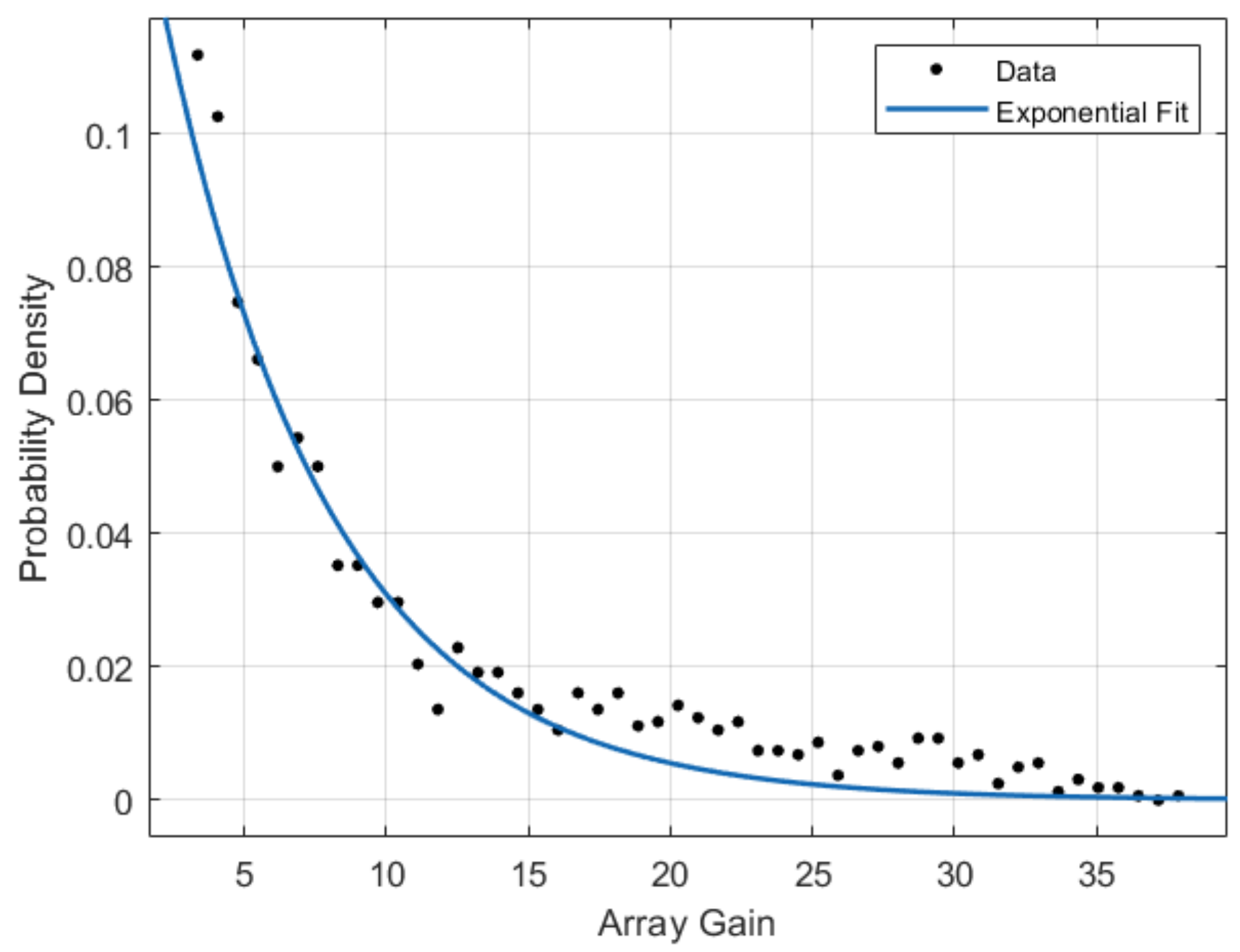
2.3.1. Array Gain
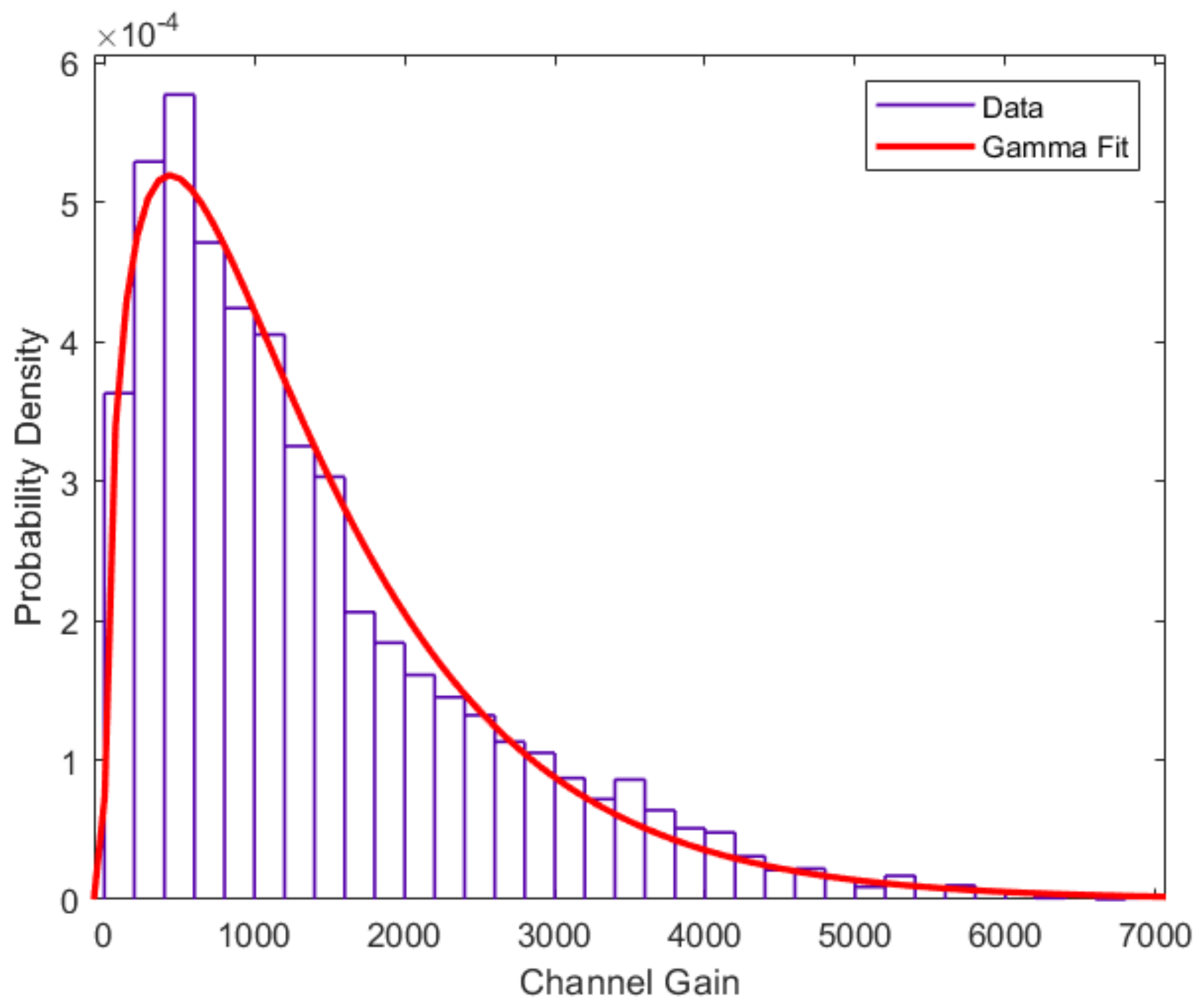
2.3.2. Channel Gain
3. Exposure Estimation
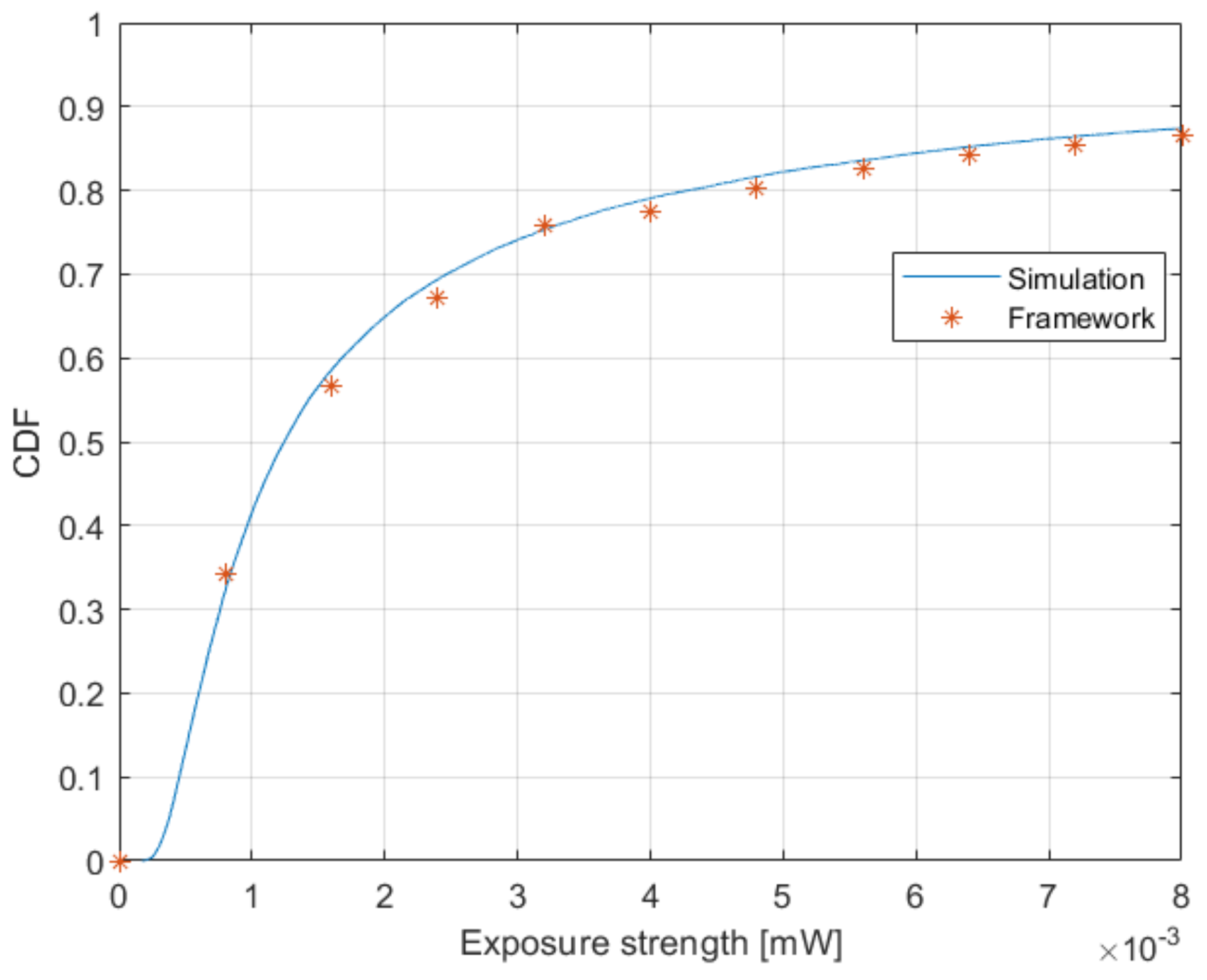
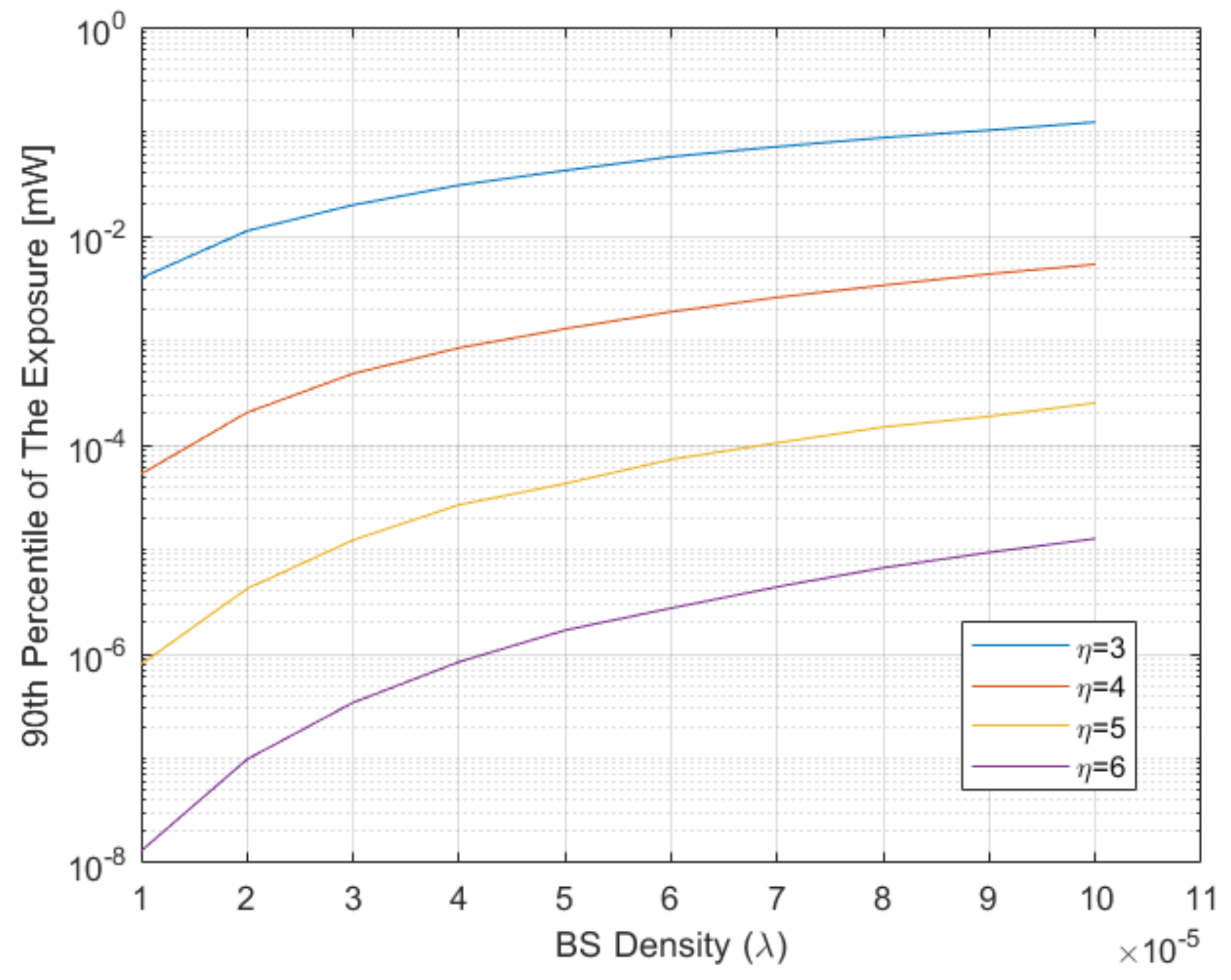
4. Numerical Results
5. Discussion
6. Conclusions
Author Contributions
Funding
Conflicts of Interest
Appendix A
Appendix B
| Abbreviation | Meaning |
|---|---|
| MIMO | Multiple Input Multiple Output |
| SNR | Signal to noise ratio |
| MISR | Mean interference to signal ratio |
| BS | Base station |
| mmWave | Millimeter Wave |
| ICNIRP | International Commission on Non-Ionizing Radiation Protection |
| PPP | Poisson point process |
| CDF | Cumulative distribution function |
| MT | Mobile terminal |
| URA | Uniformly spaced rectangular array |
| AoD | Angle of departure |
| UMI | Urban microcell |
| Probability distribution function | |
| MGF | Moment generating function |
| PCE | Polynomial chaos expansion |
| PFGL | Probability generating functional |
References
- Nitsche, T.; Cordeiro, C.; Flores, A.B.; Knightly, E.W.; Perahia, E.; Aper, I.N.P. IEEE 802.11ad: Directional 60 GHz Communication for multi-Gigabit-per-second Wi-Fi. IEEE Commun. Mag. 2014, 52, 132–141. [Google Scholar] [CrossRef]
- Rappaport, T.S.; Xing, Y.; MacCartney, G.R.; Molisch, A.F.; Mellios, E.; Zhang, J. Overview of Millimeter Wave Communications for Fifth-Generation (5G) Wireless Networks—With a Focus on Propagation Models. IEEE Trans. Antennas Propag. 2017, 65, 6213–6230. [Google Scholar] [CrossRef]
- International Commission on Non-Ionizing Radiation Protection (ICNIRP). Guidelines for Limiting Exposure to Time-Varying Electric, Magnetic and Electromagnetic Fields (100 KHz–300 GHz). Health Phys. 2020, 118, 483–524. [Google Scholar] [CrossRef] [PubMed]
- IEEE Standard for Safety Levels with Respect to Human Exposure to Electric, Magnetic, and Electromagnetic Fields, 0 Hz to 300 GHz. In IEEE Std C95.1-2019 (Revision of IEEE Std C95.1-2005/ Incorporates IEEE Std C95.1-2019/Cor 1-2019); IEEE: Piscataway, NJ, USA, 2019; pp. 1–312. [CrossRef]
- Thors, B.; Furuskar, A.; Colombi, D.; Tornevik, C. Time-Averaged Realistic Maximum Power Levels for the Assessment of Radio Frequency Exposure for 5G Radio Base Stations Using Massive MIMO. IEEE Access 2017, 5, 19711–19719. [Google Scholar] [CrossRef]
- Baracca, P.; Weber, A.; Wild, T.; Grangeat, C. A Statistical Approach for RF Exposure Compliance Boundary Assessment in Massive MIMO Systems. In Proceedings of the 22nd International ITG Workshop on Smart Antennas (WSA 2018), Bochum, Germany, 14–16 March 2018; pp. 1–6. [Google Scholar]
- Azzi, S.; Huang, Y.; Sudret, B.; Wiart, J. Surrogate Modeling of Stochastic Functions-Application to Computational Electromagnetic Dosimetry. Int. J. Uncertain. Quantif. 2019, 9, 351–363. [Google Scholar] [CrossRef]
- Aerts, S.; Verloock, L.; Bossche, M.V.D.; Colombi, D.; Martens, L.; Tornevik, C.; Joseph, W. In-Situ Measurement Methodology for the Assessment of 5G NR Massive MIMO Base Station Exposure at Sub-6 GHz Frequencies. IEEE Access 2019, 7, 184658–184667. [Google Scholar] [CrossRef]
- ETSI. Study on Channel Model for Frequencies from 0.5 to 100 GHz (3GPP TR 38.901 Version 14.0.0 Release 14); ETSI: Sophia Antipolis, France, 2017; p. 91. [Google Scholar]
- 3GPP TR 37.840—Study of Radio Frequency (RF) and Electromagnetic Compatibility (EMC) Requirements for Active Antenna Array System (AAS) Base Station. RAN#59, Release 12, 203.
- Sun, S.; MacCartney, G.R.; Rappaport, T.S. A Novel Millimeter-Wave Channel Simulator and Applications for 5G Wireless Communications. IEEE Int. Conf. Commun. 2017, 10, 1–7. [Google Scholar]
- Rappaport, T.S.; Sun, S.; Shafi, M. Investigation and Comparison of 3GPP and NYUSIM Channel Models for 5G Wireless Communications. In Proceedings of the IEEE 86th Vehicular Technology Conference (VTC-Fall), Toronto, ON, Canada, 24–27 September 2017; pp. 1–5. [Google Scholar]
- Rappaport, T.S.; Sun, S.; Mayzus, R.; Zhao, H.; Azar, Y.; Wang, K.; Wong, G.N.; Schulz, J.K.; Samimi, M.; Gutierrez, F. Millimeter Wave Mobile Communications for 5G Cellular: It Will Work! IEEE Access 2013, 1, 335–349. [Google Scholar] [CrossRef]
- Ko, J.; Cho, Y.-J.; Hur, S.; Kim, T.; Park, J.; Molisch, A.F.; Haneda, K.; Peter, M.; Park, D.-J.; Cho, D.-H. Millimeter-Wave Channel Measurements and Analysis for Statistical Spatial Channel Model in In-Building and Urban Environments at 28 GHz. IEEE Trans. Wirel. Commun. 2017, 16, 5853–5868. [Google Scholar] [CrossRef]
- Huang, J.; Wang, C.-X.; Feng, R.; Sun, J.; Zhang, W.; Yang, Y. Multi-Frequency MmWave Massive MIMO Channel Measurements and Characterization for 5G Wireless Communication Systems. IEEE J. Sel. Areas Commun. 2017, 35, 1591–1605. [Google Scholar] [CrossRef]
- Zhao, X.; Li, S.; Wang, Q.; Wang, M.; Sun, S.; Hong, W. Channel Measurements, Modeling, Simulation and Validation at 32 GHz in Outdoor Microcells for 5G Radio Systems. IEEE Access 2017, 5, 1062–1072. [Google Scholar] [CrossRef]
- Wang, C.-X.; Bian, J.; Sun, J.; Zhang, W.; Zhang, M. A Survey of 5G Channel Measurements and Models. IEEE Commun. Surv. Tutorials 2018, 20, 3142–3168. [Google Scholar] [CrossRef]
- Andrews, J.G.; Baccelli, F.; Ganti, R.K. A Tractable Approach to Coverage and Rate in Cellular Networks. IEEE Trans. Commun. 2011, 59, 3122–3134. [Google Scholar] [CrossRef] [Green Version]
- Azimi-Abarghouyi, S.M.; Makki, B.; Nasiri-Kenari, M.; Svensson, T. Stochastic Geometry Modeling and Analysis of Finite Millimeter Wave Wireless Networks. IEEE Trans. Veh. Technol. 2018, 68, 1378–1393. [Google Scholar] [CrossRef]
- El Sawy, H.; Hossain, E. On Stochastic Geometry Modeling of Cellular Uplink Transmission With Truncated Channel Inversion Power Control. IEEE Trans. Wirel. Commun. 2014, 13, 4454–4469. [Google Scholar] [CrossRef] [Green Version]
- Baccelli, F.; Giovanidis, A. A Stochastic Geometry Framework for Analyzing Pairwise-Cooperative Cellular Networks. IEEE Trans. Wirel. Commun. 2015, 14, 794–808. [Google Scholar] [CrossRef] [Green Version]
- Lu, W.; Di Renzo, M. Stochastic Geometry Modeling of MmWave Cellular Networks: Analysis and Experimental Validation. In Proceedings of the IEEE International Workshop on Measurements & Networking (M&N), Coimbra, Portugal, 10–13 October 2015; pp. 1–4. [Google Scholar]
- Di Renzo, M.; Wang, S.; Xi, X. Inhomogeneous Double Thinning—Modeling and Analysis of Cellular Networks by Using Inhomogeneous Poisson Point Processes. IEEE Trans. Wirel. Commun. 2018, 17, 5162–5182. [Google Scholar] [CrossRef]
- Wang, S.; Di Renzo, M. On the Mean Interference-to-Signal Ratio in Spatially Correlated Cellular Networks. IEEE Wirel. Commun. Lett. 2020, 9, 358–362. [Google Scholar] [CrossRef]
- Al Hajj, M.; Wang, S.; De Doncker, P.; Oestges, C.; Wiart, J. A Statistical Estimation of 5G Massive MIMO’s Exposure using Stochastic Geometry. In Proceedings of the 2020 XXXIIIrd General Assembly and Scientific Symposium of the International Union of Radio Science, Rome, Italy, 29 August–5 September 2020; pp. 1–3. [Google Scholar] [CrossRef]
- 3GPP TR 37.840—Study of Radio Frequency (RF) and Electromagnetic Compatibility (EMC) Requirements for Active Antenna Array System (AAS) Base Station. Available online: https://www.etsi.org/deliver/etsi_ts/138200_138299/138214/15.02.00_60/ts_138214v150200p.pdf (accessed on 3 December 2020).
- Venkataraman, J.; Haenggi, M.; Collins, O. Shot Noise Models for Outage and Throughput Analyses in Wireless Ad Hoc Networks. In Proceedings of the Military Communications Conference (MILCOM), Washington, DC, USA, 23–25 October 2006; pp. 1–7. [Google Scholar]
- Onggosanusi, E.; Rahman, S.; Guo, L.; Kwak, Y.; Noh, H.; Kim, Y.; Faxer, S.; Harrison, M.; Frenne, M.; Grant, S.; et al. Modular and High-Resolution Channel State Information and Beam Management for 5G New Radio. IEEE Commun. Mag. 2018, 56, 48–55. [Google Scholar] [CrossRef]
- Lenner, R.; Schilero, G.J.; Padilla, M.L.; Teirstein, A.S. A Survey on Hybrid Beamforming Techniques in 5G: Architecture and System Model Perspectives. Sarcoidosis Vasc. Diffus. Lung Dis. 2020, 19, 143–147. [Google Scholar]
- Gil-Pelaez, J. Note on the Inversion Theorem. Biometrika 1951, 38, 481. [Google Scholar] [CrossRef]
- Weisstein, E.W. Incomplete Gamma Function. MathWorld—A Wolfram Web Resource. Available online: https://mathworld.wolfram.com/IncompleteGammaFunction.html (accessed on 3 December 2020).
- Azzi, S.; Sudret, B.; Wiart, J. Sensitivity Analysis for Stochastic Simulators Using Differential Entropy. Int. J. Uncertain. Quantif. 2020, 10, 25–33. [Google Scholar] [CrossRef]
- Ringn, B. The Law of the Unconscious Statistician. 2009, pp. 1–3. Available online: http://www.maths.lth.se/matstat/staff/bengtr/mathprob/unconscious.pdf (accessed on 3 December 2020).


| Symbol | Description |
|---|---|
| Total Power Received at the center of the cell | |
| Power received from the ith BS at the center of the cell | |
| Transmitted power from all the BSs | |
| Channel and antenna gain from the ith BS to the MT | |
| Path loss experienced by the transmitted signal from the ith BS to the MT | |
| Zenith and azimuth angles in the local coordinate system centered at the origin of the array | |
| Radiation pattern and its vertical and horizontal components respectively | |
| Vertical and horizontal beamwidths of the antennas in degrees | |
| Numerically smallest number of | |
| Antenna’s front-to-back ratio | |
| Vertical and horizontal sidelobe attenuation levels | |
| Array pattern of the antenna | |
| Phase shift due to the antenna element placement | |
| Weighting factor due to the antenna element | |
| Number of horizontal and vertical antenna elements | |
| Zenith and azimuth electrical down-tilt steering angle | |
| Vertical and horizontal antenna element spacing | |
| Gamma function | |
| The Poisson point process and its density describing the BS distribution in the cell | |
| Expectation with respect to the random variable | |
| Density of the active MTs in the cell | |
| Emission probability of the BSs | |
| Mobile terminal at the center of the cell | |
| the distance between BSi and MT0 | |
| Path loss exponent assumed constant in the whole cell | |
| Moment generating function and characteristic function of the random variable | |
| CDF of the random variable | |
| Upper incomplete gamma function | |
| Lower incomplete gamma function | |
| Iid random variable describing the channel and antenna gains | |
| Generalized hypergeometric function |
| Parameter | Value |
|---|---|
| Frequency | |
| Scenario | |
| Tx Power | |
| Array type | |
| Number of elements | |
| Antenna spacing | |
| Half-Power Beamwidth | |
| Link Type | |
| RF Bandwidth | |
| User Terminal Height | |
| Base Station Height |
| Parameter | Value | Description |
|---|---|---|
| Gamma distribution shape parameter | ||
| Gamma distribution scale parameter | ||
| Exponential distribution exponent |
| Parameter | Value |
|---|---|
| Input Variable | Total Sobol Indices |
|---|---|
Publisher’s Note: MDPI stays neutral with regard to jurisdictional claims in published maps and institutional affiliations. |
© 2020 by the authors. Licensee MDPI, Basel, Switzerland. This article is an open access article distributed under the terms and conditions of the Creative Commons Attribution (CC BY) license (http://creativecommons.org/licenses/by/4.0/).
Share and Cite
Al Hajj, M.; Wang, S.; Thanh Tu, L.; Azzi, S.; Wiart, J. A Statistical Estimation of 5G Massive MIMO Networks’ Exposure Using Stochastic Geometry in mmWave Bands. Appl. Sci. 2020, 10, 8753. https://doi.org/10.3390/app10238753
Al Hajj M, Wang S, Thanh Tu L, Azzi S, Wiart J. A Statistical Estimation of 5G Massive MIMO Networks’ Exposure Using Stochastic Geometry in mmWave Bands. Applied Sciences. 2020; 10(23):8753. https://doi.org/10.3390/app10238753
Chicago/Turabian StyleAl Hajj, Maarouf, Shanshan Wang, Lam Thanh Tu, Soumaya Azzi, and Joe Wiart. 2020. "A Statistical Estimation of 5G Massive MIMO Networks’ Exposure Using Stochastic Geometry in mmWave Bands" Applied Sciences 10, no. 23: 8753. https://doi.org/10.3390/app10238753