Aerodynamic Simulation of Helicopter Based on Polyhedron Nested Grid Technology

Abstract

In this paper, a computational fluid dynamics (CFD) simulation method based on the polyhedral nested grid is developed. By comparing the simulation and test results of the hovering flow field of the Caradonna–Tung rotor, the forward flight flow field of the AH-1G rotor, the interference flow field of the Robin rotor/fuselage, and the hovering and forward flight flow field of a coaxial rotor, it is proven that the method proposed in this paper can achieve high calculation accuracy under various working conditions. The dual time-stepping method is used for the transient simulation, and the Spalart–Allmaras (S-A) turbulence model, which is widely used in aviation, is adopted in the simulation.

1. Introduction

Experimental methods and computational fluid dynamics (CFD) simulation are the main approaches to study the aerodynamic characteristics of helicopters. The experimental approach is more convincing, and sometimes more effective, for classic problems such as airframe drag reduction [1,2]. However, the experimental method has the disadvantages of long period and high investment. Meanwhile, the spatial resolution of the experimental method is low, so the detailed features inside the flow field are difficult to observe. Currently, with the improvement of CFD technology, its features of intelligence, convenience, and high precision are increasingly prominent. CFD has become an important method in the aerodynamic performance research of helicopters.

At present, CFD technology has made great contributions to aerodynamic calculation of helicopters [3,4]. In particular, the overlapping grid method [5] has attracted much attention in this field because of its unique advantages. It is suitable for almost all flight conditions of a variety of helicopters, and is currently one of the most widely used methods in this field. In addition, the sliding mesh method is often applied to helicopter hovering. It was proposed and validated by Steijl et al. [6]. For rotor CFD/CSD coupling simulation, various deformation mesh methods have been widely used, among which the spring mesh method is the most famous. Bottasso et al. [7] improved the spring mesh method and solved its shortcoming of easily forming grid deformities, so that it could deal with the problem of large deformation movement. The adaptive mesh method is widely applied in capturing the wake of the rotor vortex. This method usually uses a Cartesian grid as the background grid to adapt the background mesh conveniently. The famous American Helios project [8,9] successfully applied the adaptive mesh method to the rotor vortex wake capture and achieved remarkable effect. Jameson and Mavriplis [10] greatly improved the convergence speed of the simulation through the multigrid technology. Li et al. [11] developed a method to generate coarse grids of multiple grids, which can greatly reduce the convergence time of simulation. Nishikawa and Diskin [12] added multigrid technology to the structured overset mesh of the rotor, and the result shows that the multigrid using a structured grid can better guarantee the quality of the coarse grid, thereby improving the calculation accuracy. Shi et al. [13] developed a coupled simulation technique combining viscous wake model (VWM), computational fluid dynamics (CFD), and computational structural dynamics (CSD) to predict unsteady aerodynamic loads of rotors. Zhao et al. [14] established the CLORNS code, a robust unsteady rotor solver, to perform the transient simulation of the helicopter flow field, and the results show that the code has high accuracy in calculating aerodynamic loads of helicopter rotors. Zhou et al. [15] developed a CFD trimming method of helicopters in forward flight and achieved a good trim effect. Barakos et al. [16] proposed an unsteady actuator disk method based on surface circulation distribution, and used it to simulate the flow field of rotors in hover and forward flight states. The results show that this method is effective in capturing the major vortex structures around the disk. Tang et al. [17] proposed a method based on CFD simulation to predict the airborne spray drift and settlement under complex conditions, and applied it to the research on the downwash flow field and droplets movement law of unmanned agricultural helicopters.

As one of the fastest developing mesh technologies in recent years, polyhedral mesh technology has the advantages of fewer meshes, faster convergence speed, and higher calculation accuracy. Therefore, its application in engineering is increasingly widespread. However, there is little research on the application of this technology in helicopter flow field simulation, and the relevant literature available for reference is scarce. In this paper, polyhedral mesh technology is adopted to calculate the aerodynamic characteristics of single-rotor and coaxial-rotor helicopters under hover and forward flying conditions.

In order to prove the reliability of the simulation results, the numerical results obtained by the CFD method must be compared with the test data. Therefore, the relevant parameters of the simulation must be the same as the corresponding test conditions, including blade model, rotation speed, total distance, and so forth. Fortunately, some well-known rotor test reports provide scientists with detailed data and configurations for further study. In particular, the National Aeronautics and Space Administration (NASA) has made great contributions in this field.

2. CFD Simulation Method

2.1. Governing Equation and Solution Method

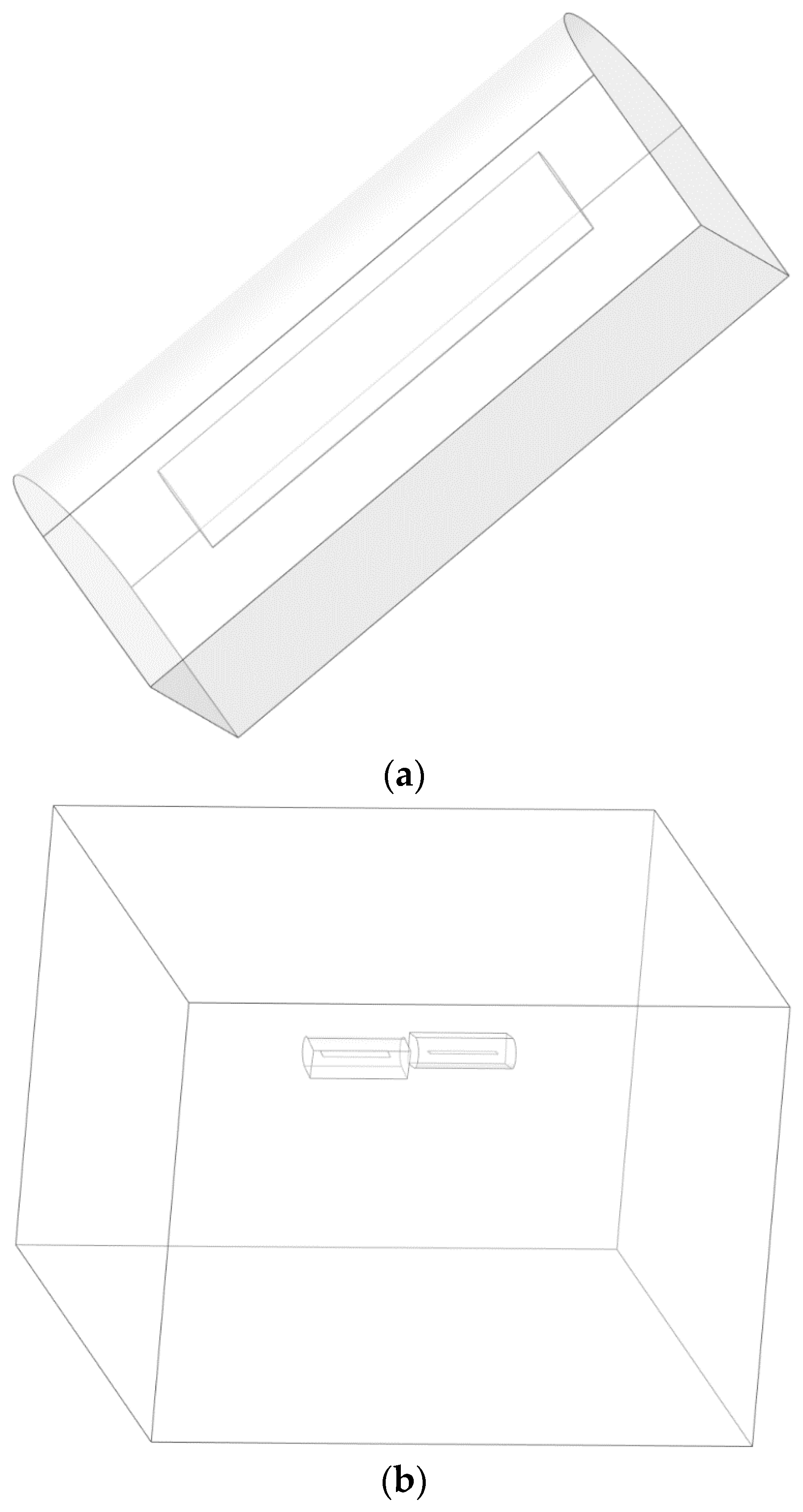
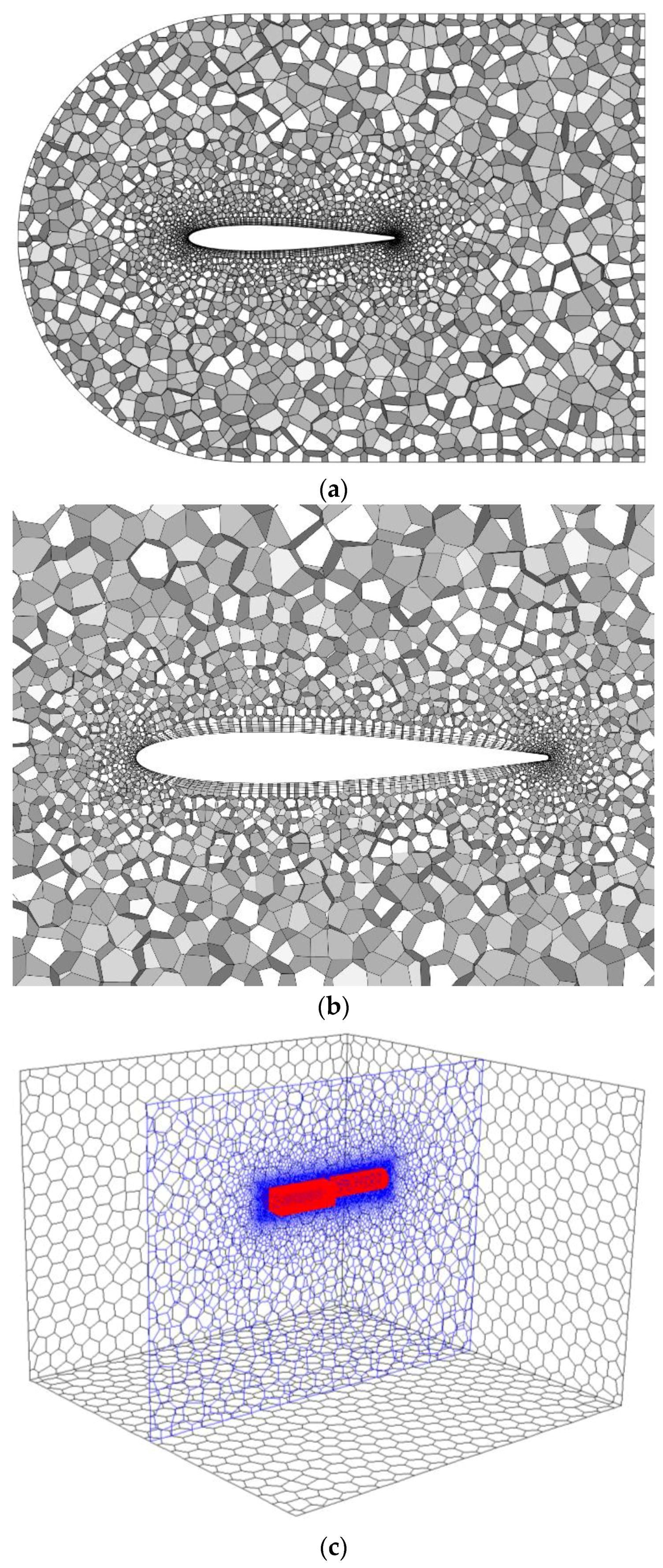
CFD simulation examples in this paper are all based on the Reynolds average Navier–Stokes (N-S) equation in the conservation form, as shown in Equation (1):

$$\frac{\partial }{\partial \mathrm{t}}{{\displaystyle \iiint }}_V\overrightarrow{W}dV+{{\displaystyle \iint }}_S\left({\overrightarrow{F}}_c-{\overrightarrow{F}}_v\right)·\overrightarrow{n}dS=0$$

(1)

where, $\overrightarrow{W}={\left[\rho ,\rho u,\rho v,\rho w,\rho e\right]}^T$ is the conservation variable, ${\overrightarrow{F}}_c=\left(f,g,h\right)$ is the convection flux, and ${\overrightarrow{F}}_v=\left(a,b,c\right)$ is the viscous flux. These parameters can be expressed as:

$$f=\left[\begin{array}{c}\rho u\\ \rho u^2+p\\ \rho uv\\ \rho uw\\ \rho ue+up\end{array}\right], g=\left[\begin{array}{c}\rho v\\ \rho uv\\ \rho v^2+p\\ \rho vw\\ \rho ve+vp\end{array}\right], h=\left[\begin{array}{c}\rho w\\ \rho uw\\ \rho vw\\ \rho w^2+p\\ \rho we+wp\end{array}\right]$$

(2)

$$a=\left[\begin{array}{c}0\\ {\tau }_{xx}\\ {\tau }_{yx}\\ {\tau }_{zx}\\ u{\tau }_{xx}+v{\tau }_{yx}+w{\tau }_{zx}-q_x\end{array}\right],b=\left[\begin{array}{c}0\\ {\tau }_{xy}\\ {\tau }_{yy}\\ {\tau }_{zy}\\ u{\tau }_{xy}+v{\tau }_{yy}+w{\tau }_{zy}-q_y\end{array}\right],c=\left[\begin{array}{c}0\\ {\tau }_{xz}\\ {\tau }_{yz}\\ {\tau }_{zz}\\ u{\tau }_{xz}+v{\tau }_{yz}+w{\tau }_{zz}-q_z\end{array}\right]$$

(3)

In the viscous flux, the stress can be expressed as:

$$\begin{gathered} {\tau }_{xx}=\frac{2}{3}\mu \left(2\frac{\partial \mu }{\partial x}-\frac{\partial \upsilon }{\partial y}-\frac{\partial w}{\partial z}\right), {\tau }_{xy}={\tau }_{yx}=\mu \left(\frac{\partial \upsilon }{\partial x}+\frac{\partial u}{\partial y}\right), q_x=-\mathsf{{\rm K}}\frac{\partial T}{\partial x} \\ {\tau }_{yy}=\frac{2}{3}\mu \left(2\frac{\partial v}{\partial y}-\frac{\partial u}{\partial x}-\frac{\partial w}{\partial z}\right), {\tau }_{yz}={\tau }_{zy}=\mu \left(\frac{\partial w}{\partial y}+\frac{\partial v}{\partial z}\right), q_y=-\mathsf{{\rm K}}\frac{\partial T}{\partial y} \\ {\tau }_{zz}=\frac{2}{3}\mu \left(2\frac{\partial w}{\partial z}-\frac{\partial u}{\partial x}-\frac{\partial v}{\partial y}\right), {\tau }_{xz}={\tau }_{zx}=\mu \left(\frac{\partial w}{\partial x}+\frac{\partial u}{\partial z}\right), q_z=-\mathsf{{\rm K}}\frac{\partial T}{\partial z} \end{gathered}$$

(4)

By introducing the relationship between pressure and temperature, the closed equations can be obtained:

$$\mathrm{p}=\mathsf{\rho }\left(\gamma -1\right)\left[e-\frac{1}{2}\left(u^2+v^2+w^2\right)\right]$$

(5)

$$\mathrm{p}=\mathsf{\rho }\mathrm{RT}$$

(6)

Among them, $\mathsf{\rho }$ represents the density of air, $\mathrm{p}$ represents the pressure, $e$ represents the total energy per unit mass of the gas, $\mu$ represents the viscosity coefficient, $\mathsf{{\rm K}}$ represents the thermal conductivity coefficient, $T$ represents the temperature, $q_x$, $q_y$, and $q_z$ represent the components of the heat flow along three directions, $\gamma$ represents the specific heat capacity, for ideal gas, $\gamma =1.4, \mathrm{R}=287.3$.

The Spalart–Allmaras (S-A) turbulence model [18] is adopted in the simulation of this paper. This model is a single-equation turbulence model, which does not derive the precise transport equation of the vortex-viscosity coefficient, but a simplified equation obtained by referring to experimental data. Thanks to Spalart’s convenience in aviation calculation, rich experience, and large amount of test data, the S-A model has been widely applied in aviation, especially in shock wave capture.

Different interpolation schemes are formed because of different discrete strategies for inviscid flux on the interface of grid cells. The Roe format [19] of flux difference splitting (FDS) in the third-order upwind format is adopted in this paper. This format has strong shock capture capability and is a method to calculate inviscid flux by approximating the Riemann solution. Due to the possibility of nonphysical understanding in the approximate Riemann solution, the entropy modified theory [20] is adopted to modify the eigenvalues in the Roe scheme.

The time discretization of the flow governing equations is based on the dual time-stepping method. Jameson [21] explained the method in detail. In this paper, the rotation of the foreground grid containing the blades is solved at 3° per time step, and each time step has 20 subiterations. It is found that the flow becomes quasi-stable after about 1.5 turns of rotation. Therefore, in order to shorten the calculation time, about three rotation cycles are calculated for each working condition.

The far field boundary adopts the nonreflective boundary condition. The nonreflective boundary is defined by Riemann invariants $R^{+}$ and $R^{-}$) [22]. The blade surface adopts the type of wall without sliding.

2.2. Grid System

In this paper, the polyhedron nested grid method is used to simulate the unsteady flow field of the helicopter. In this method, the flow field is usually divided into several regions, and each region is meshed separately. These mesh regions can overlap, nest, or overlay each other. In this way, the difficulty of mesh generation is reduced. The key technology is to build the connection relationship between the mesh regions by “hole mapping”. When it comes to the fluid problem of the body moving with time, there is also relative motion among corresponding grid blocks, so the nested grid method should be used at each time step respectively to build the relation between different mesh regions, which can be used to transport the messages at the interface needed for the CFD simulation. There are three steps to implement the overset mesh method: hole mapping, contributing cell search, and interpolation. It should be noted that in the process of generating overlapped grids, in order to ensure the interpolation accuracy at the interface of grid blocks, sufficient overlap, almost equal mesh size, and low inclination must be ensured. At the same time, the interface of the grid blocks must avoid the large physical gradient area in the flow field.

In this paper, a polyhedron nested grid method is used for simulation. It mainly contains two types of components. One is the foreground grid around the blades. In order to show the vorticity of gas as far as possible, it is necessary to encrypt the grid at the edge and tip of the blades, and add boundary layer on the blade surface. The foreground grid moves with the rotor. The other is a static background mesh nested on the foreground mesh. In order to accurately capture tip vortexes and reduce numerical dissipation, it is necessary to encrypt the area where tip vortexes are distributed in the background grid. The model of the nested system is shown in Figure 1, and the grid of the nested system is shown in Figure 2.

In order to verify the simulation technique proposed in this paper, numerical simulations are carried out on the hovering condition of the Caradona–Tung (C-T) rotor, the forward flight condition of the AH-1G rotor, the rotor/fuselage interaction flow field of Robin, and the hover and forward flight conditions of coaxial rotor. In addition, the calculated results are compared with the test data.

3. Validation of CFD Simulation Method

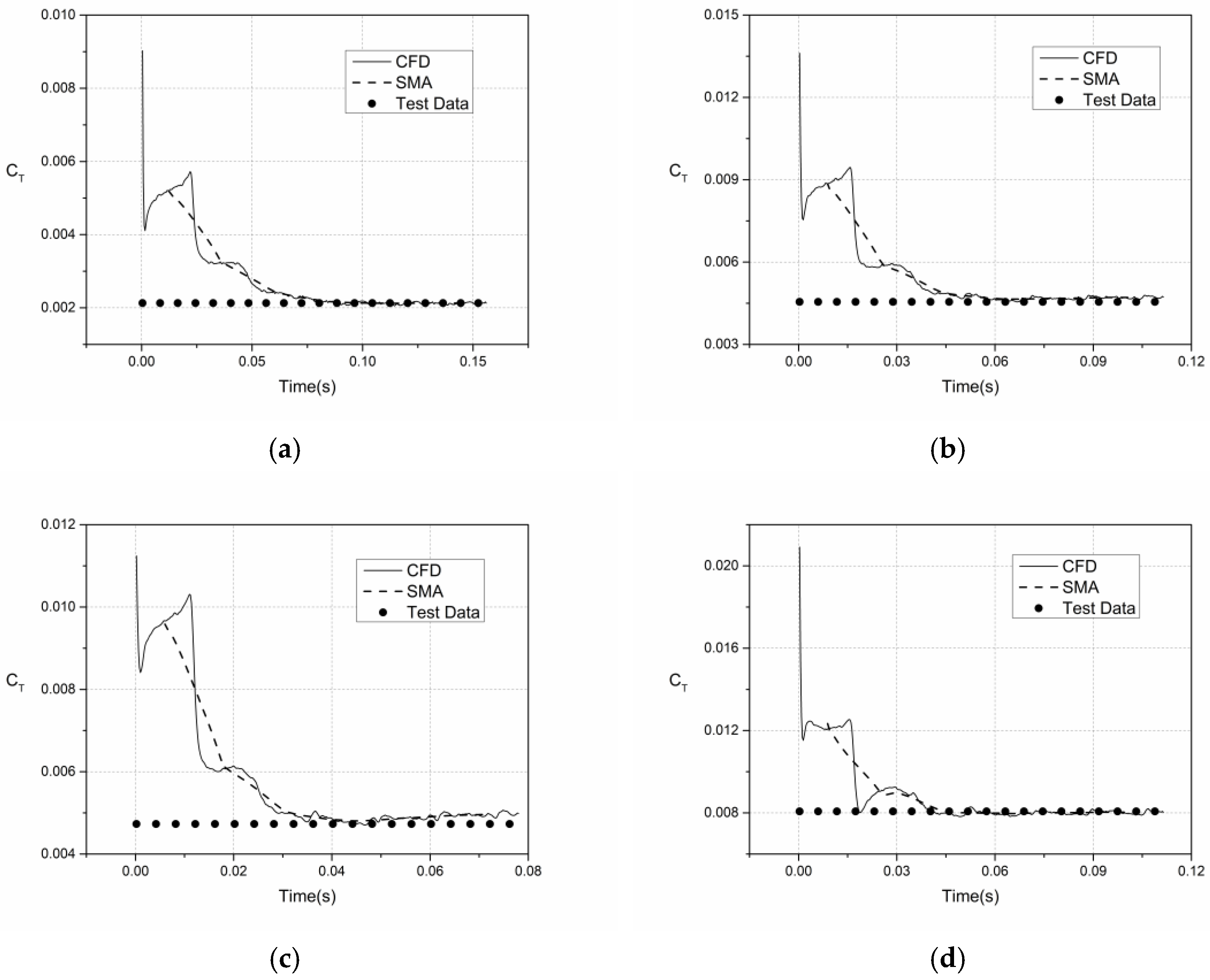
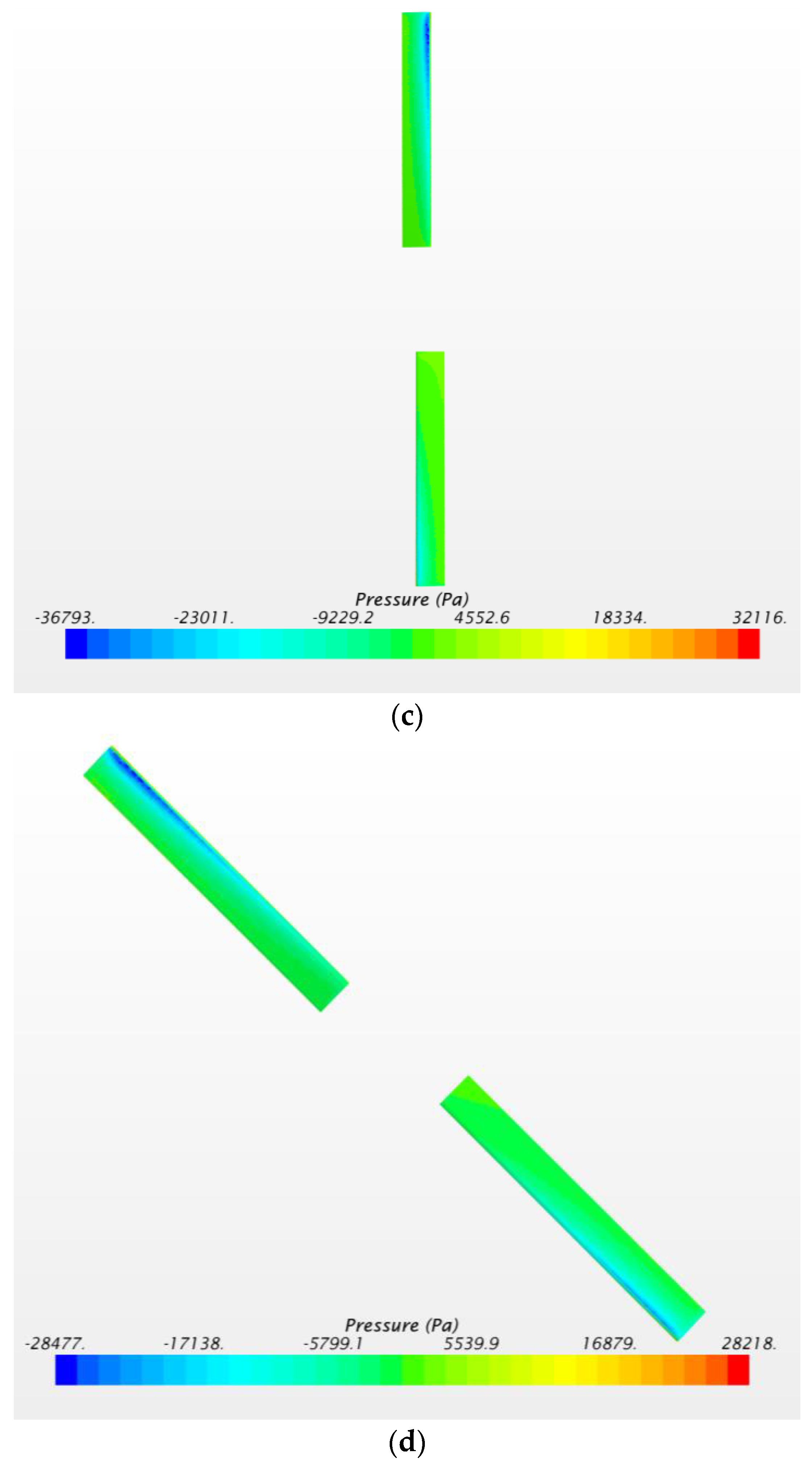
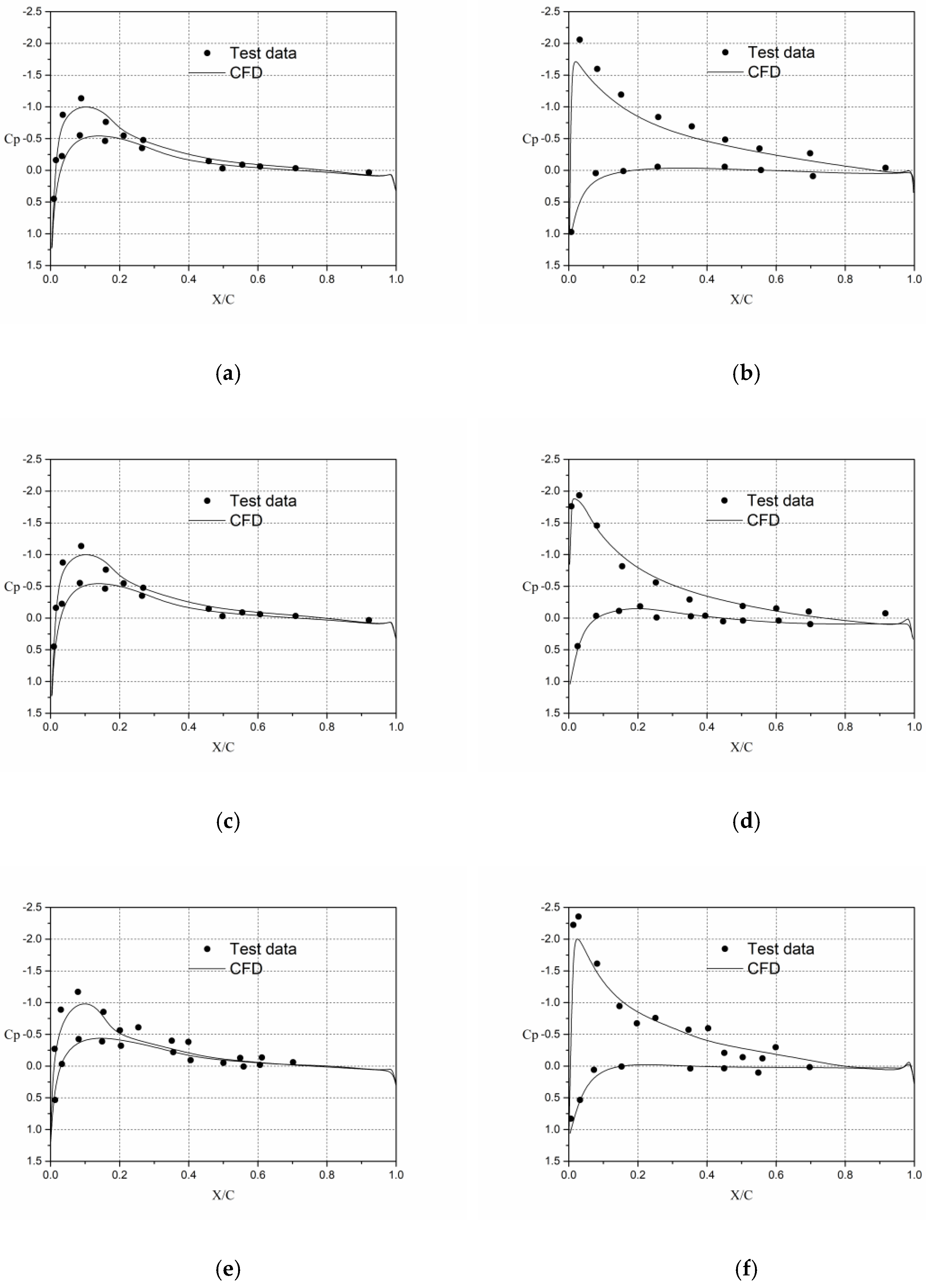
3.1. C-T Rotor in Hover

In this section, the test model of the C-T rotor [23] is taken as an example to verify the accuracy of numerical simulation in the hovering state. The detailed parameters of the C-T rotor are shown in

Table 1. Detailed parameters of C-T rotor.

Number of Blades	2
Blade radius R	1.143 m
Plane shape of blade	Rectangle
Airfoil	NACA0012
Chord length c	0.1905 m
Undercut $R_{cut}$	0.243 R
Torsion angle	0°

.

In order to verify the accuracy of the CFD method proposed in this paper, four working conditions with comprehensive test data were selected from the test report. They are: (1) $M_{tip}=0.433$, ${\theta }_c=5°$, $\mathsf{\Omega }=1250 \mathrm{RPM}$, $C_T=0.00213$; (2) $M_{tip}=0.612$, ${\theta }_c=8°$, $\mathsf{\Omega }=1750 \mathrm{RPM}$, $C_T=0.00455$; (3) $M_{tip}=0.877$, ${\theta }_c=8°$, $\mathsf{\Omega }=2500 \mathrm{RPM}$, $C_T=0.00473$; (4) $M_{tip}=0.612$, ${\theta }_c=12°$, $\mathsf{\Omega }=1750 \mathrm{RPM}$, $C_T=0.00807$. Where, $M_{tip}$ is the Mach number at the blade tip, ${\theta }_c$ is the total pitch, $\mathsf{\Omega }$ is the rotation speed, and $C_T$ is the thrust coefficient of the rotor.

Figure 3 shows the pressure contours of a blade surface in working condition 3, and Figure 4 shows the vorticity contours of the flow field in working condition 3. It can be seen from Figure 3 that there are significant shock waves near the blade tip.

Figure 5 shows the comparison between the pressure coefficient at 0.96R obtained by CFD simulation and the test data. It can be seen from this figure that the pressure coefficient distribution at 0.96R on the blade surface obtained by CFD simulation fits well with the test data.

Figure 5 shows that the pressure coefficient distribution at 0.96R on the blade surface obtained by CFD simulation fits well with the test data. To further verify the accuracy of the simulation, the thrust coefficient obtained by the simulation was compared with the test data, as shown in Figure 6:

In Figure 6, the simple moving average (SMA) is used to smooth the thrust coefficient curve. When new data are available, old data will be deleted, resulting in a curve of the average moving with the time axis. This is mainly due to the fluctuation of the monitoring results in the CFD method with the passage of physical time, which requires smoothing processing. The SMA formula is as follows:

$$\mathrm{SMA}=\frac{x_M+x_{M-1}+x_{M-2}+\cdots +x_{M-\left(n-1\right)}}{n}$$

(7)

In this case, n is 60.

Figure 6 clearly shows that as the CFD simulation goes on, the thrust coefficient of the rotor in hover tends to be stable gradually, and the stable thrust coefficient fits well with the test data, which is conducive to verifying the high accuracy of the CFD method presented in this paper. It should be pointed out that the test thrust coefficient is a constant in the test report, and for the convenience of comparison, the data points that remain unchanged over time are used for representation.

In addition, polyhedral mesh and tetrahedral mesh are used to divide the fluid domain in the simulation. The same control scale is used in the division of the two types of grids. For the background area, the global size is 0.4 m and the size surrounding the foreground area is 0.02 m, with a smooth transition between the two dimensions. For the foreground area, the global size is 0.02 m, the blade surface size is 0.005 m, and the leading and trailing edges of the blade are encrypted with a size of 0.002 m. When polyhedral grids are used, there are about 650,000 cells in a foreground region and 1.15 million cells in a background region, totaling about 2.45 million cells. When tetrahedral grids are used, there are about 2.56 million cells in a foreground region and 6.8 million cells in a background region, for a total of about 11.92 million cells. It should be noted that since there are two blades, there are two foreground areas. The same configured computer is used in the simulation to calculate the rotation of the rotor for three turns, which has a CPU model of Intel I7-9700k and a memory of 32 G. When tetrahedral mesh is used, the simulation takes about 30 h. However, when hexahedron mesh is used, the simulation takes about 18 h, which is only 60% of the time consumption of tetrahedral mesh, and their calculation results are almost the same. Therefore, it is proven that polyhedral mesh can greatly improve the efficiency of calculation while ensuring high accuracy. The same conclusion can be obtained in the following several validation examples, which proves that compared with the traditional tetrahedral mesh, the polyhedral mesh has higher computational efficiency in aerodynamic simulation of helicopters.

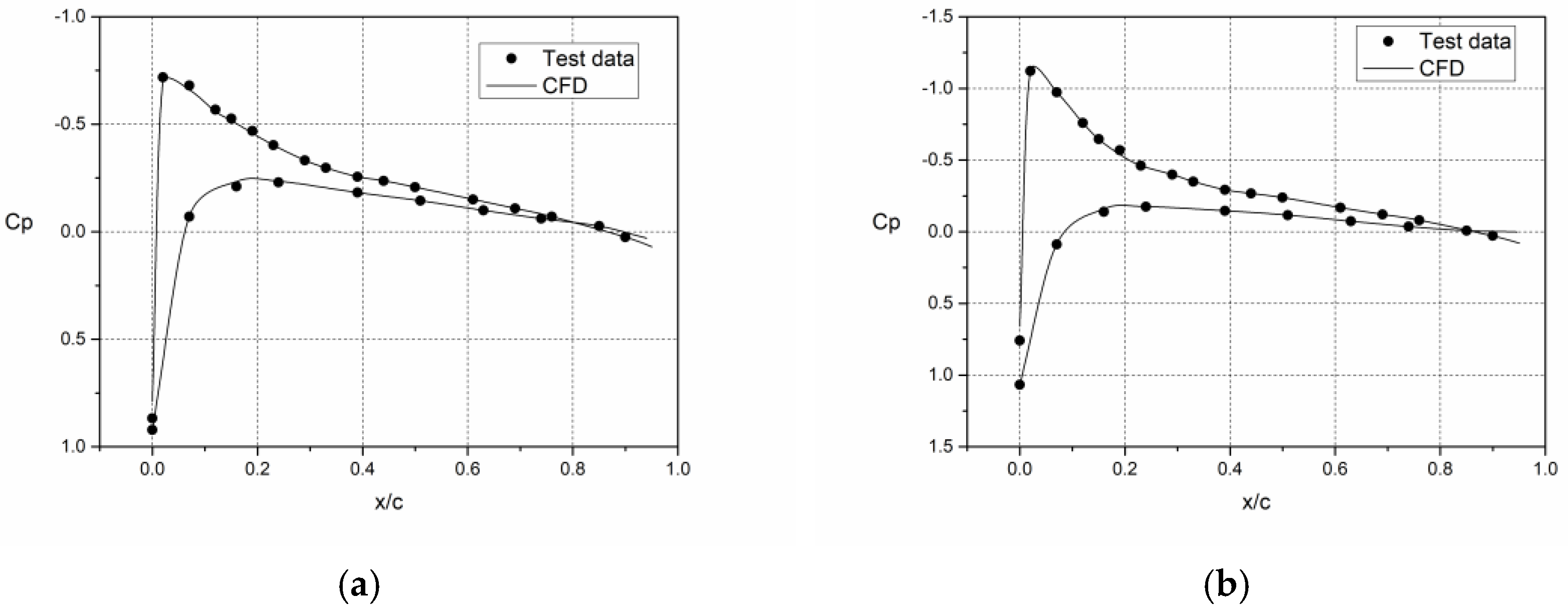
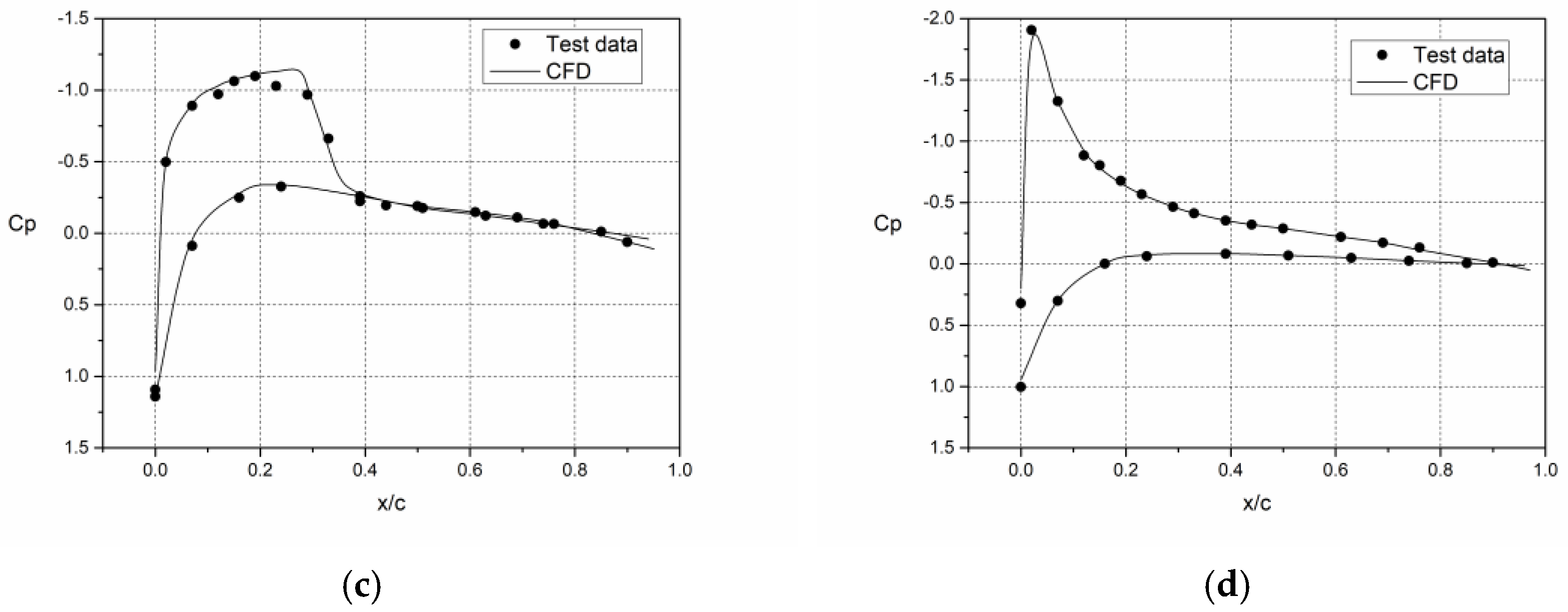
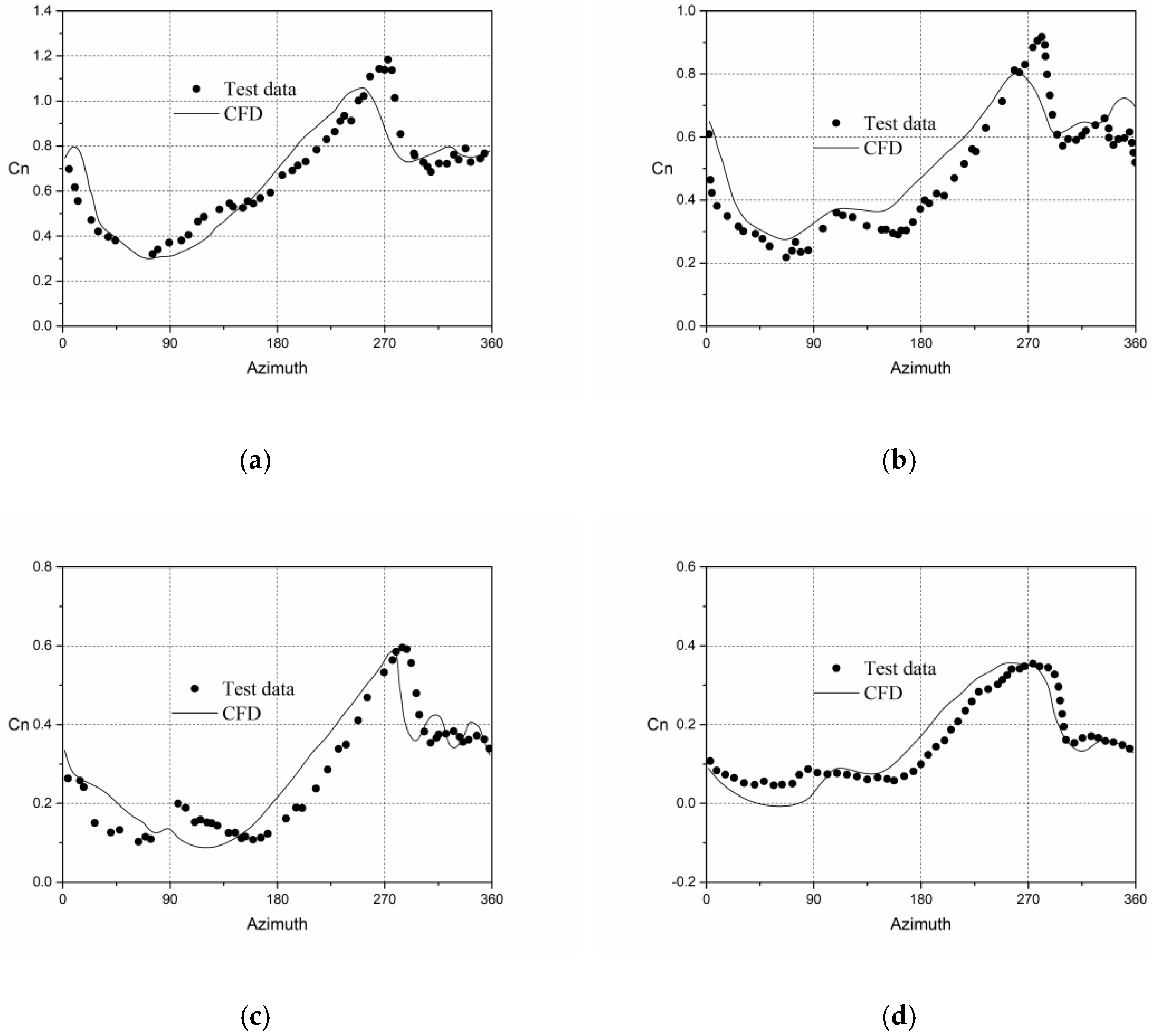
3.2. AH-1G Rotor in Forward Flight

In this section, the flight data of the AH-1G rotor [24] are chosen for CFD calculation, and the relevant parameters and flight status are shown in

Table 2. Relevant parameters and flight status of AH-1G rotor.

Number of Blades	2
Plane shape of blade	Rectangle
Airfoil	OLS
Chord length c	0.1039 m
Rotor radius R	0.958 m
Undercut $R_{cut}$	0.182 R
Torsion angle	−10°

. The test points with the tip Mach number of 0.65 and advance ratio of 0.19 are selected for simulation. The forward flight speed corresponding to this flight state is 151.864 km/h and the rotor speed is 2250 RPM. This test was selected because it has comprehensive load data, acoustic data, and blade harmonic data. In addition, the accuracy of the flight test data has been verified many times in other references [25,26,27,28].

In this flight state, the cyclic pitch motion equation of the blades is as follows:

$$\theta \left(\psi \right)=6.0°+1.7°\cos \psi -5.5°\sin \psi$$

(8)

Figure 7 shows the pressure contours of AH-1G blades at different azimuth angles obtained by CFD numerical simulation method.

According to Figure 7, it is not difficult to see that the shock waves at the blade tip in the azimuth range of 0° to 180° are more obvious than those at the azimuth range of 180° to 360°. The shock waves at the blade tip are the strongest at the azimuth angle of 90°, which is consistent with the aerodynamic theory of the helicopter.

Considering that only the overall trend of the simulation results can be seen in Figure 7, in order to more accurately judge the accuracy of the simulation, the pressure coefficient distribution of different azimuth angles and different blade profiles calculated by CFD numerical simulation method was compared with the experimental values, as shown in Figure 8.

In Figure 9, the curves of normal force coefficient with azimuth angle at four different section positions on the blade calculated by CFD simulation are given and compared with the test data. According to the data in the figure, when the azimuth angle of the advancing blade is about 70° to 90° or the retreating blade is near an azimuth of about 270°, there will be strong blade/vortex interference, resulting in abrupt change of aerodynamic force in the blade section, which makes it more difficult to simulate the rotor flow field in forward flight state.

It can be seen from Figure 8 and Figure 9 that the numerical calculation results at different azimuth angles and different blade sections are basically consistent with the test data, which proves that the CFD numerical simulation method and grid technology proposed in this paper achieve high accuracy in this type of simulation.

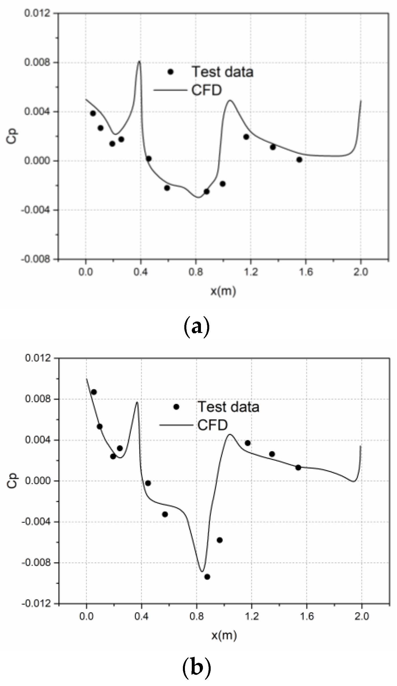
3.3. Robin Rotor/Fuselage Interference Flow Field

In this section, the interaction flow field of Robin fuselage/rotor in forward flight state is selected for calculation. The detailed data of the model are from the test report provided by NASA [29,30]. The length of the fuselage is 2 m, and the attack angle of the fuselage is 0°. The detailed parameters of the blades are shown in

Table 3. Detailed parameters of the blades in the Robin fuselage/rotor interference flow field.

Number of Blades	4
Airfoil	NACA0012
Chord length c	0.0663 m
Rotor radius R	0.8604 m
Undercut $R_{cut}$	0.24 R
Rotation speed $n$	2000 RPM
Torsion angle	−8°

.

Two forward flight states with advance ratios of 0.151 and 0.231 in the test report are selected for numerical simulation. The control parameters in these two states are shown in

Table 4. Rotor control parameters at different advance ratios.

μ	${\mathit{\theta }}_0$	${\mathit{\theta }}_{1\mathit{c}}$	${\mathit{\theta }}_{1\mathit{s}}$	${\mathit{\alpha }}_{\mathit{s}}$
0.151	10.3	−2.7	2.4	−3°
0.231	10.4	−0.4	3.8	−3°

Where μ is the advance ratio, ${\theta }_0$ is the collective pitch, ${\theta }_{1c}$ is the lateral cyclic pitch, ${\theta }_{1s}$ is the longitudinal cyclic pitch, and ${\alpha }_s$ is the attack angle of paddle.

.

Figure 10 shows the velocity contours of the Robin fuselage/rotor interference flow field within the main flow velocity range at a certain time. As the blades are in motion, the velocity contours are dynamically changing. As can be seen from this figure, the Robin fuselage is within the downwash flow range of the rotor, so there must be mutual interference of the flow field between the rotor and the fuselage. Figure 11 shows the pressure contours corresponding to the moment. Since the pressure difference range of the blade is far greater than that of the fuselage, the pressure contours of the Robin fuselage are separately shown. Figure 10 and Figure 11 show the shock wave of the forward blade and the airflow separation phenomenon of the rear blade. With the increase of the forward ratio, the downward deflection of the rotor wake decreases, and the effect of downwash flow on the fuselage is weakened.

Figure 12 compares the pressure coefficient distribution of the middle line at the top of the fuselage obtained by numerical simulation with the test data. In this figure, the X-axis represents the horizontal distance from the point on the center line of the fuselage to the fuselage head, and the Cp in the Y-axis represents the pressure coefficient at this point. By analyzing the figure, it is found that although there is a small error between the simulation data and the test data, the overall calculation accuracy is relatively high.

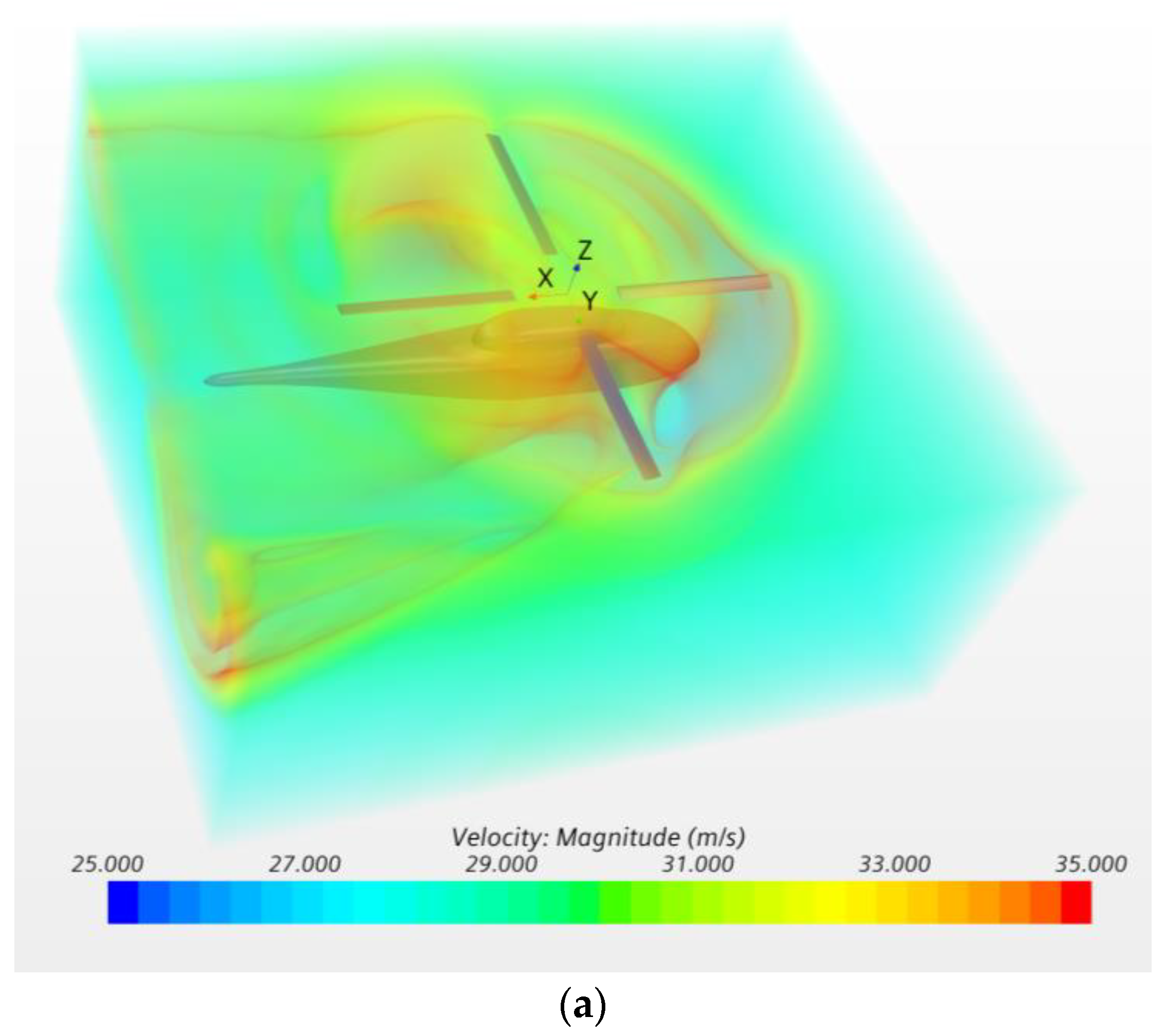
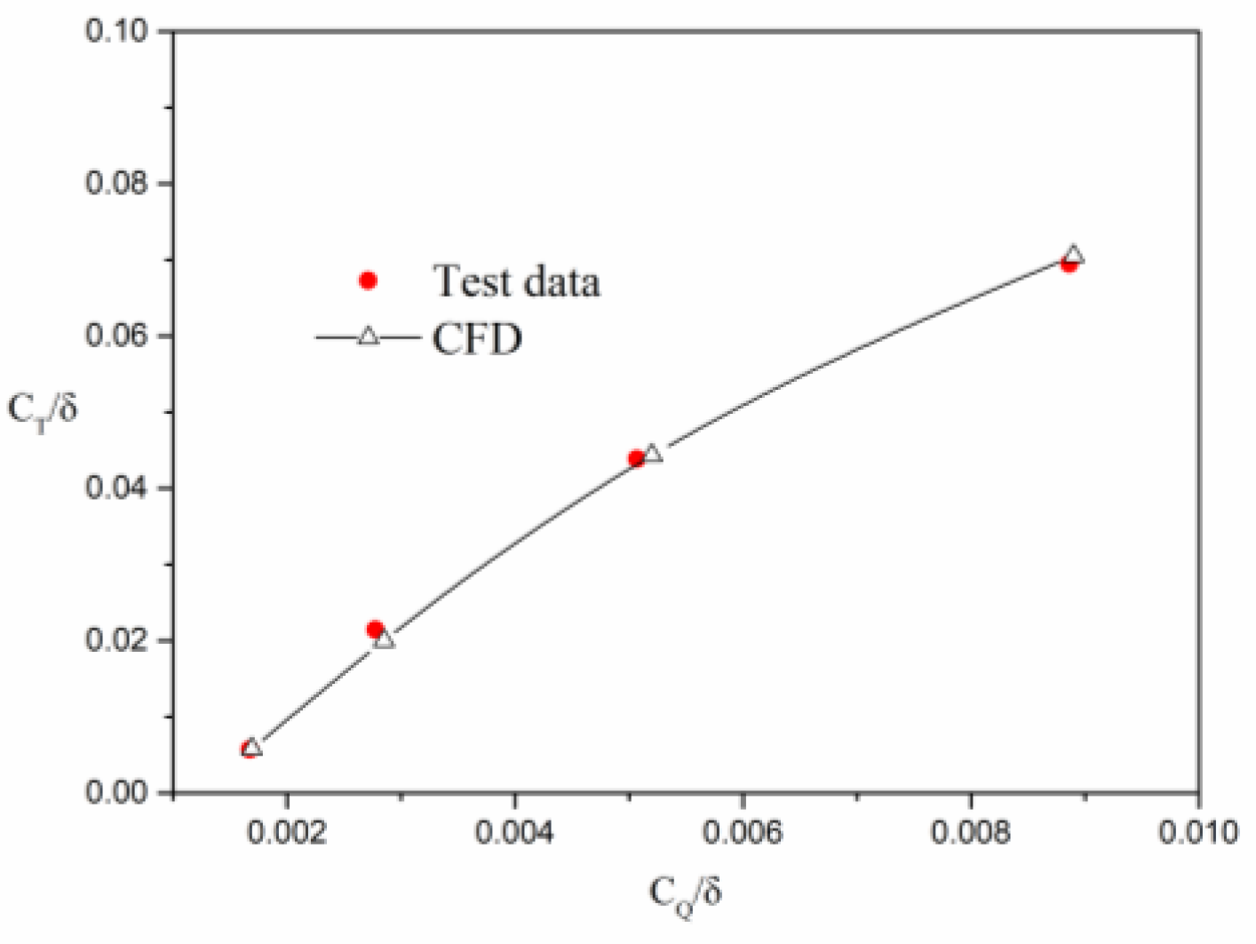
3.4. Coaxial Rotor in Hover

In this section, the flight test data [31] of a coaxial rotor provided by NASA are selected to verify the CFD simulation method and grid method proposed in this paper. In this simulation, the distance between the upper and lower rotors is 0.1 m.

The parameters of the coaxial rotor model are shown in

Table 5. Detailed parameters of the coaxial rotor.

Number of Blades	2 + 2
Plane shape of blade	Rectangle
Airfoil	NACA0012
Chord length c	0.06 m
Rotor radius R	0.38 m
Undercut $R_{cut}$	0.21 R
Rotor solidity $\delta$	0.2
Torsion angle	0°

:

Four different test states were selected for verification. The rotation speeds of the four states were all 3100 RPM, and the collective pitch of the upper and lower rotors were the same, which were 3°, 6°, 9°, and 12°. The total thrust coefficient and torque coefficient of the coaxial rotor system under each condition were calculated and compared with the test data. The calculation results are shown in Figure 13.

It can be seen from Figure 13 that the calculation values are consistent with the test data and the error is within the allowed range, thus proving that the CFD simulation method and the grid method proposed in this paper are suitable for the simulation of the interference flow field of coaxial rotors in hover and can achieve a high calculation accuracy.

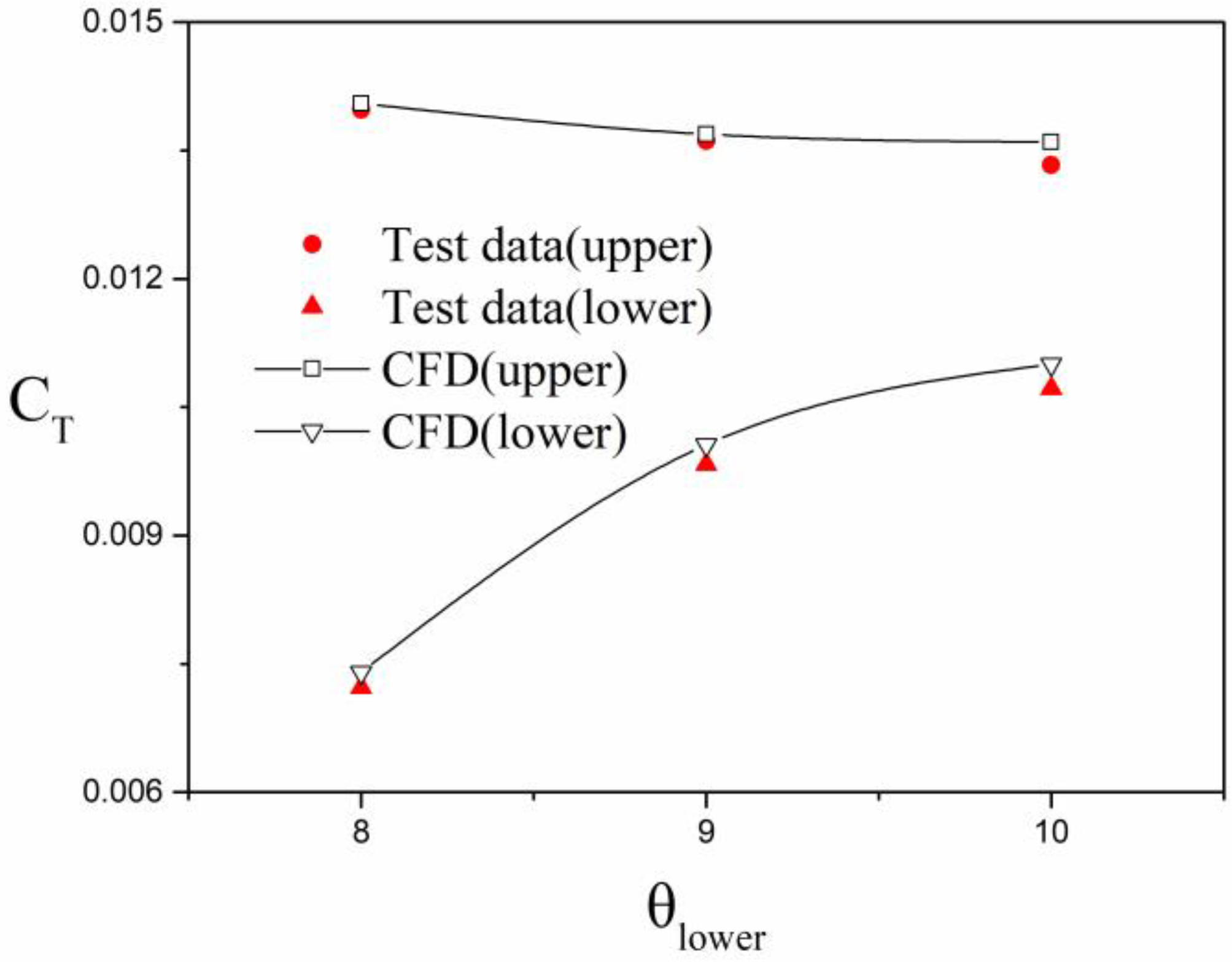
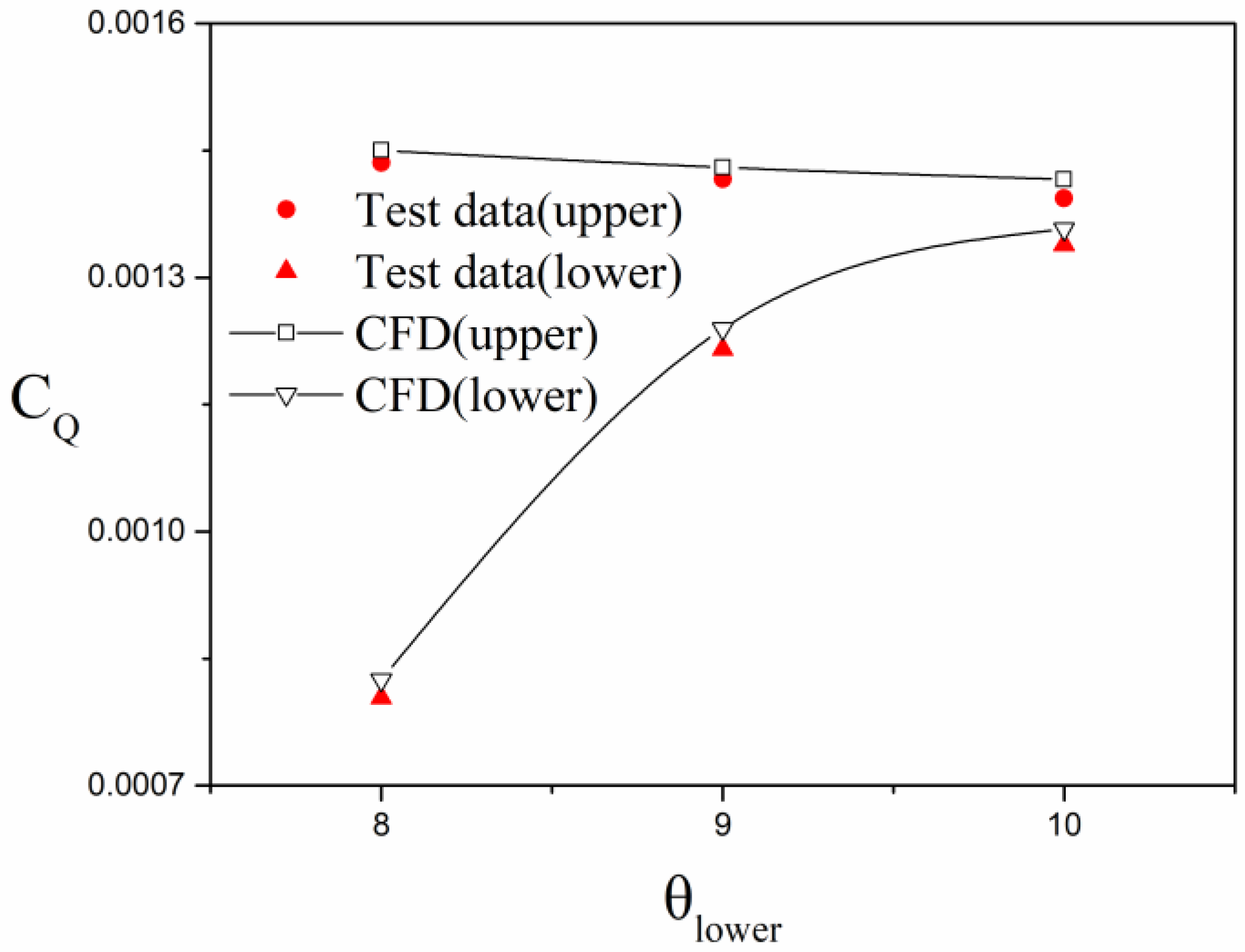
3.5. Coaxial Rotor in Forward Flight

The rotor model of Section 3.4 continues to be adopted in this section, and only the distance between the upper and lower rotors is adjusted to 0.24 m. [31] The flow field of the coaxial rotor was calculated when the advance ratio was 0.08 and the collective pitches of the upper and lower blades $\left({\theta }_{upper}, {\theta }_{lower}\right)$ were (9°, 8°), (9°, 9°), and (9°, 10°), and the thrust coefficient and moment coefficient of the calculated upper and lower rotor were compared with the test data, as shown in Figure 14 and Figure 15.

Figure 14 and Figure 15 show that the calculation results of coaxial rotors in forward flight are consistent with the test data, indicating that the polyhedral nested mesh method and CFD simulation method proposed in this paper are suitable for the numerical simulation of coaxial rotors in forward flight, and the simulation accuracy is relatively high.

4. Conclusions

A polyhedral nested grid method for CFD simulation of helicopter flow field is proposed, and verification work is carried out for a variety of models and different flight conditions. The following conclusions can be drawn:

(1)

By comparing the numerical simulation results with the test data, it is found that the numerical simulation results and the test data have a high consistency, which proves that the simulation method and grid method proposed in this paper are suitable for the aerodynamic simulation of the helicopter;

(2)

In the process of numerical simulation, polyhedral meshes can significantly reduce the number of meshes and shorten the calculation time of numerical simulation. At the same time, they can meet the requirement of high precision of helicopter flow field simulation, which has high engineering application value;

(3)

At present, there are many applications of structural grids in CFD simulation of helicopters. With the increase in the complexity of helicopter model and motion form, the time cost of structural grids becomes very high, and the new unstructured mesh represented by polyhedral mesh will undoubtedly be the research hotspot in the future.

References

1. Burley, C.L.; Brooks, T.F.; Rozier, K.Y.; Van Der Wall, B.; Richard, H.; Raffel, M.; Beaumier, P.; Delrieux, Y.; Lim, J.W.; Yu, Y.H.; et al. Rotor Wake Vortex Definition-Evaluation of 3-C PIV Results of the HART-II Study. Int. J. Aeroacoust. 2006, 5, 1–38. [Google Scholar] [CrossRef]
2. Komerath, N.M.; Smith, M.J.; Tung, C. A Review of Rotor Wake Physics and Modeling. J. Am. Helicopter Soc. 2011, 56, 22006-1–22006-19. [Google Scholar] [CrossRef]
3. Brocklehurst, A.; Barakos, G. A review of helicopter rotor blade tip shapes. Prog. Aerosp. Sci. 2013, 56, 35–74. [Google Scholar] [CrossRef]
4. Tejero, F.E.; Doerffer, P.; Szulc, O.; Cross, J.L. Numerical simulation of the tip aerodynamics and acoustics test. J. Therm. Sci. 2016, 25, 153–160. [Google Scholar] [CrossRef]
5. Benek, J.; Buning, P.; Steger, J. A 3-D chimera grid embedding technique. In Proceedings of the 7th Computational Physics Conference, Cincinnati, OH, USA, 15–17 July 1985; pp. 322–331. [Google Scholar]
6. Steijl, R.; Barakos, G. Sliding mesh algorithm for CFD analysis of helicopter rotor-fuselage aerodynamics. Int. J. Numer. Methods Fluids 2008, 58, 527–549. [Google Scholar] [CrossRef]
7. Bottasso, C.L.; Detomi, D.; Serra, R. The ball-vertex method: A new simple spring analogy method for unstructured dynamic meshes. Comput. Methods Appl. Mech. Eng. 2005, 194, 4244–4264. [Google Scholar] [CrossRef]
8. Wissink, A.; Potsdam, M.; Sankaran, V.; Sitaraman, J.; Yang, Z.; Mavriplis, D. A coupled unstructured-adaptive Cartesian CFD approach for hover prediction. In Proceedings of the AHS International 66th Annual Forum Proceedings, Phoenix, AZ, USA, 11 May 2010; pp. 1300–1317. [Google Scholar]
9. Lim, J.; Wissink, A.; Jayaraman, B.; Dimanlig, A. Application of adaptive mesh refinement technique in Helios to blade-vortex interaction loading and rotor wakes. In Proceedings of the 67th Annual Forum of the American Helicopter Society International, Virginia Beach, VA, USA, 3–5 May 2011; pp. 228–250. [Google Scholar]
10. Jameson, A.; Mavriplis, D. Finite volume solution of the two-dimensional Euler equations on a regular triangular mesh. AIAA J. 1986, 24, 611–618. [Google Scholar] [CrossRef]
11. Li, Z.; Wang, Z.; Cao, W.; Yao, L. An aspect ratio agglomeration multigrid for unstructured grids. Int. J. Numer. Methods Fluids 2013, 72, 1034–1050. [Google Scholar] [CrossRef]
12. Nishikawa, H.; Diskin, B. Development and Application of Parallel Agglomerated Multigrid Method for Complex Geometries. In Proceedings of the 20th AIAA Computational Fluid Dynamics Conference, Honolulu, HI, USA, 27–30 June 2011; pp. 2514–2528. [Google Scholar]
13. Shi, Y.; Xu, Y.; Xu, G.; Wei, P. A coupling VWM/CFD/CSD method for rotor airload prediction. Chin. J. Aeronaut. 2017, 30, 204–215. [Google Scholar] [CrossRef]
14. Zhao, Q.; Zhao, G.; Wang, B.; Wang, Q.; Shi, Y.; Xu, G. Robust Navier-Stokes method for predicting unsteady flowfield and aerodynamic characteristics of helicopter rotor. Chin. J. Aeronaut. 2018, 31, 214–224. [Google Scholar] [CrossRef]
15. Zhou, C.; Chen, M. Computational fluid dynamics trimming of helicopter rotor in forward flight. Adv. Mech. Eng. 2020, 12, 1–13. [Google Scholar] [CrossRef]
16. Barakos, G.; FitzGibbon, T.; Kusyumov, A.; Kusyumov, S.; Mikhailov, S. CFD simulation of helicopter rotor flow based on unsteady actuator disk model. Chin. J. Aeronaut. 2020, 33, 2313–2328. [Google Scholar] [CrossRef]
17. Tang, Q.; Zhang, R.; Chen, L.; Deng, W.; Xu, M.; Xu, G.; Li, L.; Hewitt, A. Numerical simulation of the downwash flow field and droplet movement from an unmanned helicopter for crop spraying. Comput. Electron. Agric. 2020, 174, 105468. [Google Scholar] [CrossRef]
18. Spalart, P.; Allmaras, S. A one-equation turbulence model for aerodynamic flows. Rech. Aerosp. 1994, 1, 5–21. [Google Scholar]
19. Roe, P. Approximate Riemann Solvers, Parameter Vectors, and Difference Schemes. J. Comput. Phys. 1997, 135, 250–258. [Google Scholar] [CrossRef] [Green Version]
20. Harten, A.; Hyman, J.M. Self adjusting grid methods for one-dimensional hyperbolic conservation laws. J. Comput. Phys. 1983, 50, 235–269. [Google Scholar] [CrossRef]
21. Jameson, A. Time dependent calculations using multigrid, with applications to unsteady flows past airfoils and wings. In Proceedings of the 10th Computational Fluid Dynamics Conference, Honolulu, HI, USA, 24–27 June 1991. [Google Scholar]
22. Jameson, A.; Schmidt, W.; Turkel, E. Numerical solution of the Euler equations by finite volume methods using Runge Kutta time stepping schemes. In Proceedings of the 14th Fluid and Plasma Dynamics Conference, Palo Alto, CA, USA, 23–25 June 1981; AIAA Journal: Reston, VA, USA. [Google Scholar] [CrossRef] [Green Version]
23. Caradonna, F.X.; Tung, C. Experimental and analytical studies of a model helicopter rotor in hover. Vertica 1981, 5, 149–161. [Google Scholar]
24. Cross, J.F.; Watts, M.E. Tip Aerodynamics and Acoustics Test: A Report and Data Survey; NASA Langley Technical Report Server: Washington, DC, USA, 1988. Available online: https://ntrs.nasa.gov/citations/19890008208 (accessed on 5 September 2013).
25. Ahmad, J.; Duque, E.P.N. Helicopter rotor blade computation in unsteady flows using moving overset grids. J. Aircr. 1996, 33, 54–60. [Google Scholar] [CrossRef]
26. Yang, Z.; Sankar, L.N.; Smith, M.J.; Bauchau, O. Recent Improvements to a Hybrid Method for Rotors in Forward Flight. J. Aircr. 2002, 39, 804–812. [Google Scholar] [CrossRef]
27. Hernandez, F.; Johnson, W. Correlation of airloads on a Two-Bladed helicopter rotor. In Proceedings of the International Specialist Meeting on Rotorcraft Acoustics and Rotor Fluid Dynamics, Philadelphia, PA, USA, 15–17 October 1991. [Google Scholar]
28. Ramachandran, K.; Schlechtriem, S.; Caradonna, F.X.; Steinhoff, J.S. Free-Wake Computation of Helicopter Rotor Flowfield in Forward Flight. In Proceedings of the AIAA 23rd Fluid Dynamics, Plasma Dynamics and Lasers Conference; Orlando, FL, USA, 6–9 July 1993, NASA Langley Technical Report Server: Washington, DC, USA, 1993. Available online: https://ntrs.nasa.gov/citations/19930064256 (accessed on 16 August 2013).
29. Raymond, E.M.; Susan, A.G. Steady and Periodic Pressure Measurements on a Generic Helicopter Fuselage Model in the Presence of a Rotor; NASA Langley Technical Report Server: Washington, DC, USA, 2000. Available online: https://ntrs.nasa.gov/citations/20000057579 (accessed on 7 September 2013).
30. Phelps, A.E.; Berry, J.D. Description of the US Army Small-Scale 2-Meter Rotor Test System; NASA Langley Technical Report Server: Washington, DC, USA, 1987. Available online: https://ntrs.nasa.gov/citations/19870008231 (accessed on 5 September 2013).
31. Coleman, C.P. A Survey of Theoretical and Experimental Coaxial Rotor Aerodynamic Research; NASA Langley Technical Report Server: Washington, DC, USA, 1997. Available online: https://ntrs.nasa.gov/citations/19970015550 (accessed on 6 September 2013).
Figure 1. The nested system model. (a) The foreground area surrounding the blades. (b) Assembly drawing of the foreground area and background area.
Applsci 10 08304 g001
Figure 2. Blade motion nested mesh. (a) Grid section of the foreground area. (b) The boundary layer region of the foreground grid section. (c) Assembly system of the nested grid.
Applsci 10 08304 g002
Figure 3. Pressure contours of a blade in working condition 3.
Applsci 10 08304 g003
Figure 4. Vorticity contours of flow field in condition 3.
Applsci 10 08304 g004
Figure 5. Surface pressure coefficients of C-T rotor at 0.96R profile in hover. (a) M t i p = 0.433 ,   θ c = 5 ° . (b) M t i p = 0.612 , θ c = 8 ° . (c) M t i p = 0.877 ,     θ c = 8 ° . (d) M t i p = 0.612 , θ c = 12 ° .
Applsci 10 08304 g005aApplsci 10 08304 g005b
Figure 6. C-T rotor thrust coefficient curve with physical time. (a) M t i p = 0.433 , θ c = 5 ° . (b) M t i p = 0.612 , θ c = 8 ° . (c) M t i p = 0.877 , θ c = 8 ° . (d) M t i p = 0.612 , θ c = 12 ° .
Applsci 10 08304 g006
Figure 7. Pressure contours of AH-1G blades at different azimuth angles. (a) Azimuths of 0 and 180 degrees. (b) Azimuths of 45 and 225 degrees. (c) Azimuths of 90 and 270 degrees. (d) Azimuths of 135 and 315 degrees.
Applsci 10 08304 g007aApplsci 10 08304 g007b
Figure 8. Pressure coefficient of AH-1G rotor varies with azimuth and blade section. (a) ψ = 30 ° ,   r R = 0.60 . (b) ψ = 180 ° ,   r R = 0.60 . (c) ψ = 90 ° ,   r R = 0.91 . (d) ψ = 270 ° ,   r R = 0.91 . (e) ψ = 90 ° ,   r R = 0.97 . (f) ψ = 270 ° ,   r R = 0.97 .
Applsci 10 08304 g008
Figure 9. Normal force coefficients of AH-1 rotor vary with azimuth angles. (a) r/R = 0.60. (b) r/R = 0.75. (c) r/R = 0.91. (d) r/R = 0.99.
Applsci 10 08304 g009
Figure 10. Velocity contours of Robin fuselage/rotor interference flow field. (a) μ = 0.151. (b) μ = 0.231.
Applsci 10 08304 g010aApplsci 10 08304 g010b
Figure 11. Pressure contours of Robin fuselage/rotor interference flow. (a) Fuselage/rotor, μ = 0.151. (b) Fuselage, μ = 0.151. (c) Rotor, μ = 0.151. (d) Fuselage/rotor, μ = 0.231. (e) Fuselage, μ = 0.231. (f) Rotor, μ = 0.231.
Applsci 10 08304 g011aApplsci 10 08304 g011bApplsci 10 08304 g011c
Figure 12. Pressure coefficient distribution in the center line of the top fuselage. (a) μ = 0.151. (b) μ = 0.231.
Applsci 10 08304 g012
Figure 13. Variation of thrust coefficient and torque coefficient with collective pitch of the coaxial rotor in hover.
Applsci 10 08304 g013
Figure 14. The thrust coefficient of the upper and lower rotors varies with the collective pitch of the lower rotor.
Applsci 10 08304 g014
Figure 15. The moment coefficient of the upper and lower rotors varies with the collective pitch of the lower rotor.
Applsci 10 08304 g015