Acoustic Scattering Models from Rough Surfaces: A Brief Review and Recent Advances

Abstract

This paper proposes a brief review of acoustic wave scattering models from rough surfaces. This review is intended to provide an up-to-date survey of the analytical approximate or semi-analytical methods that are encountered in acoustic scattering from random rough surfaces. Thus, this review focuses only on the scattering of acoustic waves and does not deal with the transmission through a rough interface of waves within a solid material. The main used approximations are classified here into two types: the two historical approximations (Kirchhoff approximation and the perturbation theory) and some sound propagation models more suitable for grazing observation angles on rough surfaces, such as the small slope approximation, the integral equation method and the parabolic equation. The use of the existing approximations in the scientific literature and their validity are highlighted. Rough surfaces with Gaussian height distribution are usually considered in the models hypotheses. Rather few comparisons between models and measurements have been found in the literature. Some new criteria have been recently determined for the validity of the Kirchhoff approximation, which is one of the most used models, owing to its implementation simplicity.

1. Introduction

The scattering of waves from rough surfaces is an important phenomenon in diverse areas of science, such as optics, geophysics, communications, acoustics, hydraulics [1], elastodynamics for non-destructive testing, etc. For instance, in the particular case of ultrasonic waves, scattering from rough surfaces leads to many applications in non-destructive testing [2], in underwater acoustics for high resolution ultrasonic sonars [3] and for medical sciences [4,5]. The modeling of such phenomena is a century-old and still active research topic.

Scattering models of acoustic waves from rough surfaces could be classified into analytical models, numerical ones and combinations of both analytical and numerical methods. However, such a classification is rather ambiguous, since some analytical models (usually called semi-analytical) employ numerical calculations and since some numerical methods start from analytical approximations. The current review focuses on analytical or semi-analytical methods and the validity of each method will be emphasized as well as some applications examples. Some analytical methods are presented or used in the following in more detail: the Kirchhoff approximation (KA), the perturbation theory (PT), the integral equation (IE) method, the parabolic equation (PE) method and the small slope approximation (SSA). The Kirchhoff and PT methods represent early classical approaches but are still very often employed in the literature, notably the Kirchhoff one. The other methods represent more modern approaches which have larger domains of validity but are more complex and therefore more difficult to implement or can lead to a higher calculation time. All the previously cited methods have been found to be amongst the most common in the literature and many of the other methods of the literature are based on or have much in common with these approaches.

This review focuses thus only on the scattering of acoustic waves and does not deal with the transmission through a rough surface of waves within a solid material. Indeed the models used in acoustics are often also employed in elastodynamics. For instance, the elastic Kirchhoff model has been devised to deal with rough defects [6,7,8] and to take into account mode-conversions between compressional and shear waves. A variety of analytical models involving reflection and transmission waves (for instance through a rough fluid–solid interface), such as the phase screen approximation [9,10,11,12] and Kirchhoff theory, have been developed to understand the elastic fields in solids or scattered from different embedded scatterers.

Several reviews of scattering from rough surfaces exist in the literature, notably in general physics (diverse areas of sciences) for random rough surfaces [13,14,15] or in electromagnetism [16,17]. The main review describing works in acoustic scattering from rough surfaces has been written by Ogilvy in the 80s [18], although its review does not only deal with acoustics. This review has notably summarized the two classical approximations (Kirchhoff and the perturbation theory) but it is now out of date: since this review, important models have been devised for grazing incidence or observation, such as the small slope approximation, and new criteria have notably been established for defining the validity of the Kirchhoff approximation, which is probably the most used analytical model for roughness scattering. Some other textbooks also deal with acoustic scattering from rough surfaces notably in the view of ocean applications [19,20]. At Ogilvy’s time, the accuracy of Kirchhoff approximation came from Thorsos’ work [21] and was determined by the ratio of the height correlation length L of the random rough surface to the wavelength. It is also the case in Voronovich’s more recent textbook (see Figure 1) [20], where approximations KA, PT and SSA are all said to require this ratio less than a constant in order to be valid; another different criterion has even been proposed for radar applications [22]. Recent studies—described in the present review and based on numerical calculations—have shown for elastodynamic problems that the accuracy of the Kirchhoff theory should depend on the parameter σ²/L (σ and L being the RMS surface height and the height correlation length). Kirchhoff is considered accurate when this parameter is smaller than an upper bound c depending on the wavelength: (σ²/L < c). Kirchhoff accuracy is also dependent on incidence and scattering angles. In the recent years new developments or comparisons of the previous methods have also been proposed in the literature and for different applications, such as non-destructive evaluation (NDE), underwater acoustics or even medicine.

Section 1 of the current paper is devoted to the parametrization of rough surfaces, Gaussian height distribution being usually assumed in modeling. The two historical approximations (Kirchhoff and the perturbation theory) are then described (Section 2) as well as their use in the scientific literature, their validity and an application example for non-destructive testing. Then, more modern approaches with larger domains of validity (notably suitable for grazing observation angles and generally having applications for underwater acoustics) are presented in Section 3.

2. Rough Surfaces Parametrization

This section is devoted to mathematical methods used to characterize randomly rough surfaces. A rough surface is described using its height deviation from a mean smooth surface. Hereafter are presented the statistical distributions (height and correlation functions) and associated parameters usually employed to properly define the rough surface properties. We will here take the example of Gaussian height distributions since most of the used models of rough surface scattering assume such a distribution. However, although many surfaces (both natural and engineered) exhibit Gaussian height distributions, there are also many others that do not [23,24]. Examples of generating non-Gaussian rough surfaces can be found in the literature [25,26].

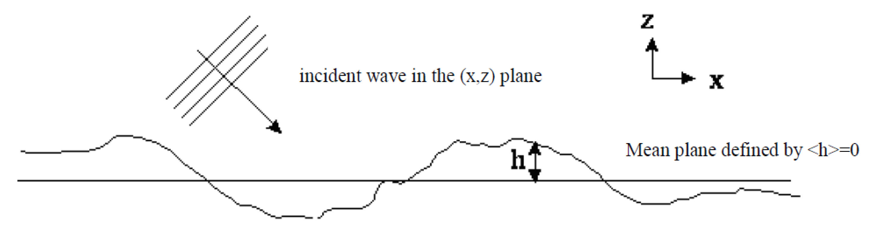
2.1. Statistical Properties

Surface roughness is described here as the variation of height $z=h(x,y)$ above or below a mean surface. <h>, the average of the height variation over the surface, is by definition 0. h is assumed to be random and described statistically using parameters such as the RMS height and spatial correlation lengths. In the theory presented hereafter and developed by Ogilvy [6,27], it is assumed that the height distribution is well represented by a Gaussian.

The probability of any measured height being between h and h + dh above or below the mean plane is then given by p(h) dh, where:

$$p\left(h\right)=\frac{1}{\sigma {\left(2\pi \right)}^{\frac{1}{2}}}{e}^{-\raisebox{1ex}{$\hspace{0.17em}{h}^2$}\!\left/ \!\raisebox{-1ex}{$2{\sigma }^2$}\right.}$$

(1)

where $\sigma$ is the RMS height:

$$\sigma ={\left[\langle h^2\rangle \right]}^{\frac{1}{2}}$$

(2)

Random rough surfaces show some spatial correlation, as the height at a location is not totally independent of surrounding heights. This may be described by the correlation function of a surface, $C\left(R\right)$ where:

$$C\left(R\right) =\frac{1}{{\sigma }^2}\langle h\left(r\right)h(r +R)\rangle$$

(3)

which represents the extent to which the surface height at any one point $r$ is, on average, related to the surface height at point r + $R$ away. Gaussian functions are often used as an approximation of the correlation of real surfaces. Assuming the same Gaussian correlation in every direction, C can be written:

$$C\left(R\right) =e^{\_\raisebox{1ex}{$R$}\!\left/ \!\raisebox{-1ex}{$L^2$}\right.}$$

(4)

where $L$ is called the correlation length of the surface. Anisotropic correlation functions can also be used to describe surface with a direction-dependent correlation. Such surfaces often occur in practice in industrial structures, as roughness can be generated in anisotropic manner during the manufacturing process.

2.2. Generation Process of an Individual Gaussian Rough Surface

The method of generating these surfaces is described in detail in [6,27]. It first generates uncorrelated random numbers with a Gaussian distribution of zero mean and specified RMS value. Then, it performs a moving average with weights that ensure that the correlation function is Gaussian with the desired correlation length. The following weights yield a surface with two independent lengths $L_x^{}$ and $L_y^{}$ in the two perpendicular directions:

$$W_{ij} =e^{-2\left[{\left(i\Delta x\right)}^2/L_x^2+{\left(i\Delta y\right)}^2/L_y^2\right]}$$

(5)

$\Delta x$ is the interval between adjacent surface points in the x direction and $\Delta y$ is the corresponding interval in the y direction. The surface correlation function is defined for a reference point $(x_0,y_0)$ by:

$$C\left(x,y\right) =\frac{\langle h(x_0,y_0)h(x_0+x,y_0+y)\rangle }{\langle h^2\rangle }$$

(6)

The weights given in Equation (5) yield the following surface correlation function:

$$C\left(x,y\right) =e^{-\left[x^2/L_x^2+y^2/L_y^2\right]}$$

(7)

This method allows generating different realizations of random surfaces sharing the same statistical parameters (see Figure 7d for an application example).

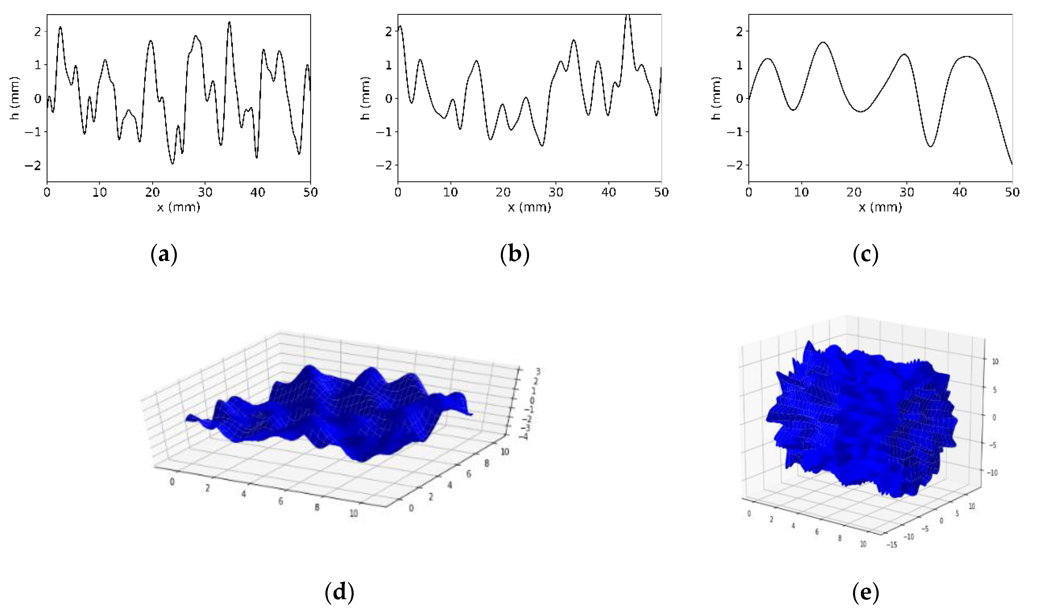
2.3. Implementation Example for Generation of an Individual Gaussian Rough Surface

The parameters to be chosen as inputs for the parametrization of a Gaussian rough surface are:

-

The RMS surface height: $\sigma ={\left[\langle h^2\rangle \right]}^{\frac{1}{2}}$. As the height is defined with zero mean ($\langle h\rangle$ = 0), the standard deviation $\sigma ={\left[\langle {\left(h-\langle h^2\rangle \right)}^2\rangle \right]}^{\frac{1}{2}}$ of the height is equal to the RMS height $rms(h)={\left[\langle h^2\rangle \right]}^{\frac{1}{2}}$: $\sigma ={\left[\langle {\left(h-\langle h\rangle \right)}^2\rangle \right]}^{\frac{1}{2}}={\left[\langle h^2\rangle \right]}^{\frac{1}{2}}=rms(h)$.

-

The correlation lengths, $L_x^{}$ and $L_y^{}$, along the local axes x and y.

The number of mesh points of the rough surface along the local axes x and y has then to be automatically fixed by the chosen mesh algorithm. The previously described Gaussian rough surface model is currently implemented for planar and cylindrical surfaces in 3D computations, and for their linear cross-sections in 2D, in the CIVA software [28] (platform for non-destructive evaluation simulation [29,30,31,32,33]). Examples of generated surfaces for small specimens with relatively high roughness are shown in Figure 1.

3. Historical Approximations

This section deals with the perturbation and Kirchhoff approximations. Both have been extensively applied to rough surfaces and have their own strengths and weaknesses. Other approaches will be dealt with in later sections.

Figure 2 shows the geometry used in this section for rough surface scattering.

We consider a rough surface whose roughness is defined by z = h(x,y) where h is the height variation above or below the mean plane, z = 0. The xz plane contains the incident wavevector.

3.1. The Perturbation Theory

The perturbation theory (PT) assumes some restrictive hypotheses on the local height h and gradient $\nabla h$ at points of a rough surface:

$$k\left|h\right|<<1$$

(8)

$$\left|\nabla h\right|<<1$$

(9)

k being the incident wavevector modulus.

It is assumed that if previous conditions are satisfied, the roughness is weak compared to acoustic wavelength and slowly varies. It expresses the scattered field at an observation point $r$ as an expansion series:

$$\psi (r)={\psi }^{inc}(r)+{\displaystyle \sum _{n=0}^{\infty }{\psi }_n^{sc}(r)}$$

(10)

where ${\psi }^{inc}$ is the incident wave field and ${\psi }_n^{sc}$ is the nth-order approximation to the scattered field. The n = 0 term is the scattered field from a smooth surface. Then the main principle of the perturbation Theory consists in assuming that the boundary conditions may be expanded in a Taylor series about the mean plane z = 0. Mathematically, the boundary conditions on the rough surface expressed as:

$$f\left(x,y,z\right)=0$$

(11)

where f can be, for instance, the acoustical pressure for Dirichlet conditions—which can be expanded in a Taylor series about the mean plane z = 0 as follows:

$$f\left(x,y,z\right){|}_{z=h(x,y)}=f\left(x,y,z\right){|}_{z=0}+h\frac{\partial f}{\partial z}{|}_{z=0}+\frac{h^2}{2}\frac{{\partial }^{2}f}{\partial z^2}{|}_{z=0}+\dots .$$

(12)

Some applications of the perturbation theory consider first scattering from canonical rough surfaces [18]. For instance for the Lamb’s problem (scattering from a surface excited by a load force applied at one particular surface point) [34], the solution is expressed as convolution integrals evaluated only for a triangular irregularity of small height compared to its width and to the wavelength. The application of PT to random rough surfaces leads to consider separately a mean coherent contribution and an incoherent one. For the coherent part, reflection and transmission coefficients are determined. For the incoherent part, the mean intensity of the scattered field is calculated [35]. The determined first-order PT term can be substituted back into the Helmholtz scattering formula to iteratively deduce higher order terms.

Blakemore [36] has then presented a Perturbation Theory at the first order for a fluid/solid interface. PT simulations in backscattering for rigid and elastic solids are very close except at the vicinity of the Rayleigh angle as shown in Figure 3.

In this region a small peak in the intensity of the incoherently scattered field is predicted, consistent with experiment. Nevertheless, in the case of the proposed experimental validation in pulse echo configuration [37] (Figure 4), Kirchhoff prediction (not shown here) are about 3 dB lower than PT one at backscattering angles theta = 40°, and 5.5 dB lower at theta = 70°.

Some applications and references of PT for scattering from fluid/fluid, fluid/solid interfaces and fluid/stratified layers [38,39,40] for inhomogeneous media [41,42] can be found in the literature, generally for ocean applications. An acoustic model in the time domain based on first-order perturbation theory for scattering from layered sediments has recently been proposed [43].

Only a few authors have been interested in the scattering from canonical non-planar rough targets. Notably Bjorno [44,45] recently investigated the scattering problem for an elastic rough sphere. He developed in that case a second-order perturbation model. He compared the scattering patterns obtained versus the adimensional wave-number ka and for different values of the ratio of the rms height to the sphere radius with its perturbation solution to the classical acoustic scattering solution for a smooth sphere [46,47]. Measurements of the backscattering response of a cast iron sphere versus ka led to a good experimental validation of the proposed model: the roughness yields a decrease in the backscattered amplitude notably for large ka values. The accuracy is limited to small values of the ratio rms height to wavelength.

Note also, for instance, a recent development in electromagnetism of the perturbation theory for a slightly deformed cylinder [48].

We also have to cite the phase perturbation method [49,50] in which the phase (rather than the field) is expanded in a series of different orders in kh. This theory exhibits links with both PT and Kirchhoff [51]. A validation [52] of the phase perturbation method has been proposed and has consisted in comparing its results to numerical ones in a region where PT and Kirchhoff are found ineffective. The phase perturbation method is found to work well in such a region except for low grazing observation angles. However, applications of this new theory seem not numerous and are more focused on radar cross sections calculations [53].

Although the perturbation approach can take into account of the scattering and re-radiation of Rayleigh waves, it appears possibly more restrictive than the Kirchhoff method in its range of applicability. The perturbation method is notably an approach valid for low roughness (when compared to acoustic wavelength). Several validations of the PT are provided in the next sections; they also show that PT is rather accurate far from the specular direction.

3.2. The Kirchhoff Approximation

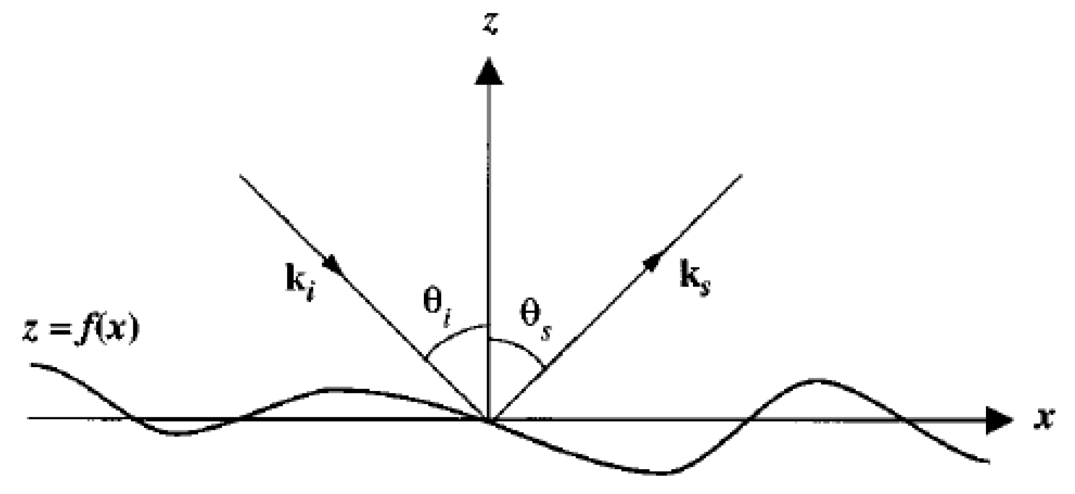
3.2.1. Theory and History

The main hypothesis of the Kirchhoff approximation (also referred to as the physical optics approximation) is to assume that each point of the surface behaves as if it belonged to the infinite tangent plane to this surface. Then it is practical to employ geometrical acoustics to approximate the exact fields on the local surface: the field on the illuminated part of surface is the sum of the incident field and the field reflected by the local tangential plane. This supposed surface field is then propagated far from the surface using a propagator (called Green function). Indeed the scattered far field is expressed by the way of an integral over the flaw surface (the Kirchhoff–Rayleigh integral) whose integrand is—for the example of Dirichlet conditions—the product of the Green function by the derivative of the geometrical field on the flaw surface. For complex incident fields or scatterer shapes, this integral is evaluated numerically.

The Kirchhoff approximation has been extensively used to model scattering of waves in optics (early introduced by Meecham [54]), electromagnetism [55,56], acoustics, etc. In both acoustics [57] and elastodynamics [58,59], the Kirchhoff approximation also has the advantage in dealing with anisotropic materials and impedant surfaces [57].

Note that when doing an asymptotic evaluation of the KA integral on a finite surface, the KA resulting leading terms describe the reflected waves, and the other terms describe diffracted waves by the surface edges which have the same nature (cylindrical or conical wave fronts) but not the same amplitude as those predicted by the geometrical theory of diffraction (GTD) [55,60]. The main advantage of the Kirchhoff approximation is to provide finite results for the scattered field in the whole space, contrary to GTD [61,62,63,64,65]. One of the main inconveniences of the Kirchhoff approximation (KA) is its incorrect quantitative prediction of edges diffraction, since the approximation of the surface field by the geometrical field is invalid near the edges. To handle this drawback, the physical theory of diffraction (PTD) has been proposed in electromagnetism [66], acoustics [59,67] and elastodynamics [68,69,70] and compared to other uniform scattering models [67,70,71].

In the literature, the Kirchhoff approximation has been studied by different authors. A review has been carried out by Ogilvy [18]. The first one to introduce the Kirchhoff approximation is Eckart [72].

Ogilvy [27] has well described the theory for 1D rough profile (Figure 2) and Dirichlet conditions (soft interface) extending Eckart’s works. De Billy et al. proposed a Kirchhoff-based theory extended to shadowing effects for the backscattering of acoustic waves by randomly rough surfaces [37]. De Billy et al. employed in fact the potential-method formulation developed by Welton which showed by iterating the scattering integral equation that the scattered pressure can be expressed as a series: the first term corresponds to the singly and the others to the multiply scattered field components. De Billy et al. considered only the first term. Their experimental validations of their model using Gaussian rough (liquid–solid interfaces) surfaces have shown that the experimental measurements of the intensity backscattered by randomly rough interfaces (liquid–solid) are in good agreement with the theory until 40° backscattering angles (with respect to the normal to the mean plane). Nevertheless, an anomaly has been observed in Kirchhoff’s predictions for the Rayleigh’s angle of incidence. In fact, to model the impedance surfaces used in their experimental validations, they simply add a reflection coefficient as a factor inside the Kirchhoff integral, and for backscattering the local reflection coefficient is the one at normal incidence for a plane surface: this formalism does not take into account any mode conversion in the elastic medium and is unable to predict any perturbation at the different critical angles. Following de Billy’s works which studied the Kirchhoff approximation using monochromatic plane waves, Imbert [73] has proposed a Kirchhoff model in time domain for 2D rough profiles and Neumann conditions (rigid interface).

We can sum up the main steps of Kirchhoff approximation application as follows:

1.

Use of the Helmholtz equation: the scattered field is:

$$\psi \left(r\right)={\psi }^{inc}\left(r\right)+{{\displaystyle \int }}_{S_0}\left(\psi \left(r_0\right)\frac{\partial G\left(r,r_0\right)}{\partial n_0}-G\left(r,r_0\right)\frac{\partial \psi \left(r_0\right)}{\partial n_0}\right)d{S}_{0 } .$$

(13)

The equation is also called Green theorem and $G\left(r,r_0\right)=\frac{e^{ik\left|r-r_0\right|}}{4\pi \left|r-r_0\right|}$ is called the Green function, where $r_0$ is a current point on the scattering rough surface $S_0$ and r the observation point. The field in the fluid medium can be obtained thanks to the knowledge of its value on the surface $S_0$.

2.

Boundary Conditions on the rough surface: Ogilvy [27] considered for instance Dirichlet boundary conditions (soft case) so that $\psi (r_0)$ = 0. So one term in the previous Green integral disappears:

$$\psi \left(r\right)={\psi }^{inc}\left(r\right)+{{\displaystyle \int }}_{S_0}\left(-G\left(r,r_0\right)\frac{\partial \psi \left(r_0\right)}{\partial n_0}\right)d{S}_0$$

(14)

3.

Kirchhoff approximation: the tangential plane approximation enables to approximate the value of $\frac{\partial \psi \left(r_0\right)}{\partial n_0}$ inside the previous integral.

4.

Far field approximation: the integrand value can be simplified by assuming $kr$ >> 1, $k$ being the wave number.

5.

Projection of integration on the rough surface on the smooth surface: this projection involves the gradients of the roughness.

6.

Incorporation of a shadow function to approach auto-shadowing: Wagner [74] has proposed to incorporate a shadow function inside the Kirchhoff integral to take into account shadowing effects.

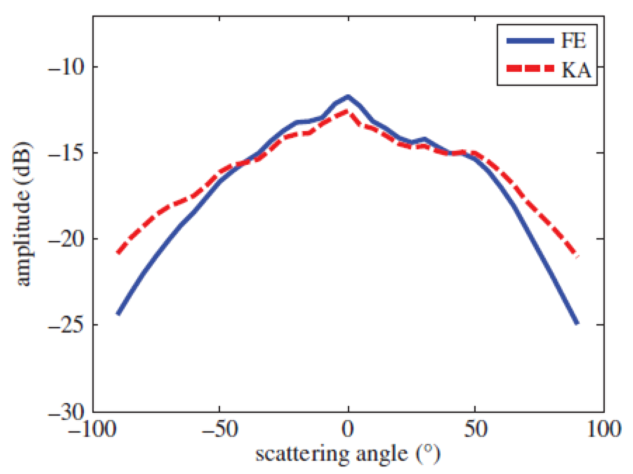
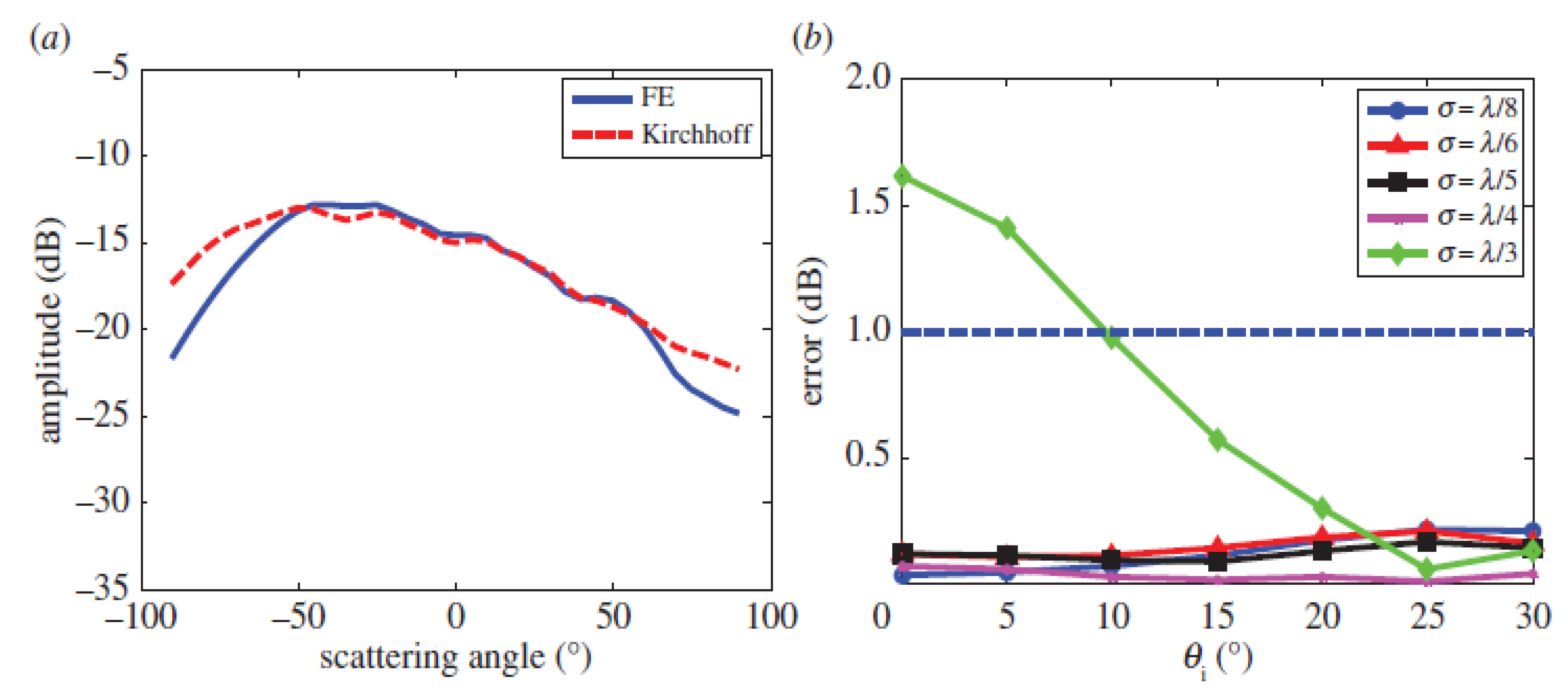
Note that the Kirchhoff approximation is mainly used to predict far-field scattering; a model has been proposed to evaluate the scattering pattern in near-field [75] after the interaction of an acoustic wave with a rough interface.

3.2.2. Validity

Historically KA has been considered—in the point of view of its local tangential plane assumption—as accurate when the rough surface can be seen planar by the incident wave. In Ogilvy’s review [7], KA is thus said valid for kr_c cos³ θi >> 1, with r_c the surface local radius of curvature and θi the incident angle. This historical criterion forgets that multiple scattering and shadowing effects are not taken into account in KA leading to large errors for grazing incidences or higher roughness.

KA prediction has been compared to Integral Equation (IE) results by Thorsos [21] for 1D rough profiles. Thorsos proposed to use the surface correlation length $L$ as main parameter for defining the Kirchhoff validity away from the low grazing angle region: KA is said to be accurate for a correlation length greater than the wavelength or even for lower correlation lengths if shadowing effects are not important. We notice this first criterion proposed by Thorsos at this step is too simple and not involve the rms height. In the low grazing angle region some examples of validation with comparison to another methods are given in next Section 4; at low grazing angles, additional validity dependence enters through the RMS slope which is for Gaussian rough surfaces: $s=\tan \gamma =\surd 2\frac{\sigma }{L}$ i.e., the rms height is now involved. However, at shorter correlation lengths, the needed shadowing correction proposed by Thorsos becomes greater to improve Kirchhoff prediction at low grazing angles in the case of backscattering.

Note that in order to improve its prediction for low grazing angles, Chapman [76] provided an improved Kirchhoff formula (using a smoothing special function) notably by including the correlation length of the scattering surface into the reflection coefficient. The modification impact is not noticeable since shadowing and multiple scattering will dominate for low grazing angles. Chapman showed that the PT and KA results differ except in the limit of infinite correlation length (smooth surface).

Shi et al. [77] recently proposed for elastic materials (also for shear waves [78,79]) and for compressional waves a different surface parameter than the surface correlation length $L$ used by Thorsos, a function σ²/L of both L and σ, to define a criterion when the KA use is valid. They found that, with a normal incidence angle θi = 0°, KA is valid with a scattering angle −70° < θs < 70°and when σ²/L ≤ c, the constant upper bound c being in two dimensions 0.20 λp and in three dimensions 0.14 λp (λp being the compressional wavelength). Figure 5 shows a comparison between KA and a finite element (FE) method for a 2D case when σ²/L~c. A small incidence angle of 30° can improve the KA accuracy when σ²/L exceeds c as in the case shown in Figure 6. We can however regret that the numerical evaluation of this proposed criterion was limited to small incidences angles: however, this criterion is likely to be suitable for many NDE configurations for which incidence is close to normal. A study of this criterion near grazing incidence should also be useful.

As said in the introduction, another different KA validity criterion has been proposed for radar applications [22] and is also based on numerical calculations: it is given by Equation (1) in [22] (see also their Figure 3, Kirchhoff being called the scalar approximation) and ensures a KA validity for L²/σ more than a constant times the wavelength and a condition kL > 6 is also associated. We find the condition on L²/σ very disbelieving and in contradiction with the previously cited studies and also that given by Voronovich (σ/L < C and large kL; see Figure 1.1 in [20]). The condition kL >6 is also found in other references as [52]. Notably, Figure 2 in [52] represents the stated validity of first-order perturbation theory and KA in kσ–kL space obtained for bistatic scattering cross sections simulation: PT is said valid for small kσ < 2 to 4 depending on kL value, KA valid for kL > 6 and both KA and first-order PT needs σ/L < C (C being a constant value).

In our opinion, this KA condition kL > 6 is too restrictive for many applications, such as non-destructive evaluation, which often employs near specular observation inspection. First, we previously study or carry out numerical comparisons of KA simulation for cracks of finite size L inspected with longitudinal waves in solids with numerical methods: the method of optimal truncation (MOOT) [80] and a finite element method (FEM) [81,82]. These comparisons with MOOT [83] and FEM [69,84] both show that KA is valid for near specular observation inspection for kL > 2. Shi et al. [77] did not propose a validity criterion on kL (but only the condition on σ²/L); they nevertheless obtained an acceptable disagreement of 2dB (see their Figure 10 [77]) for kL = π/2 (corresponding to L = λp/4) and for an important roughness σ = λp/4 = L equal to the correlation length. It is a pity that that they did not provide numerical validations below kL = π/2.

Our conclusive opinion is that for many applications using rather near specular observation and non-grazing incident angles, two criteria can be used for KA validity: σ²/L ≤ Cλp and kL > 1 or 2. For more important observation angles to the normal the criterion on kL and the constant C value are likely to be a little more restrictive: Zhang [85] using 2D FEM calculations recently showed that KA can be considered accurate for kL > π and for incidence and scattering angles over the range from −80° to 80°.

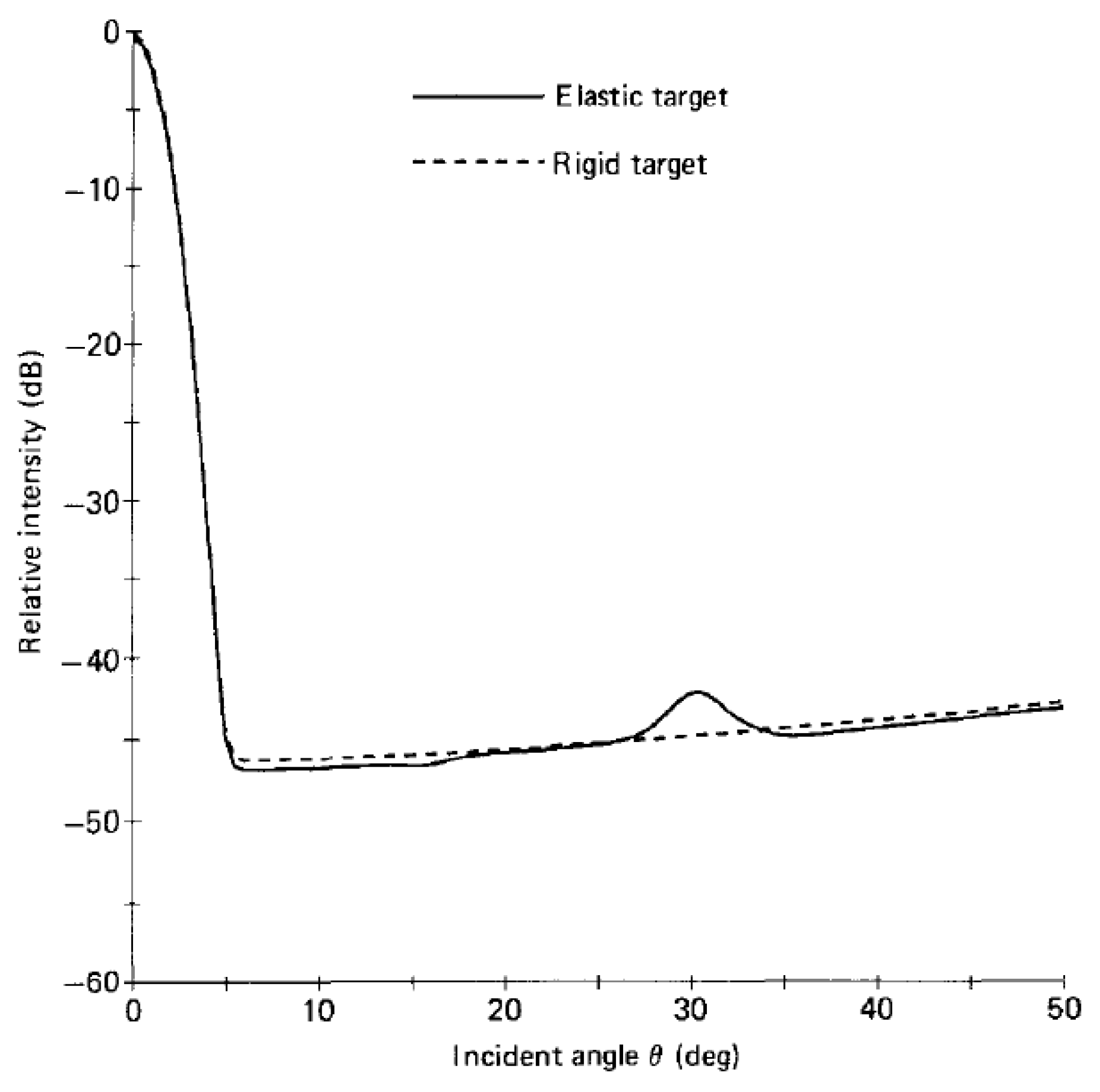
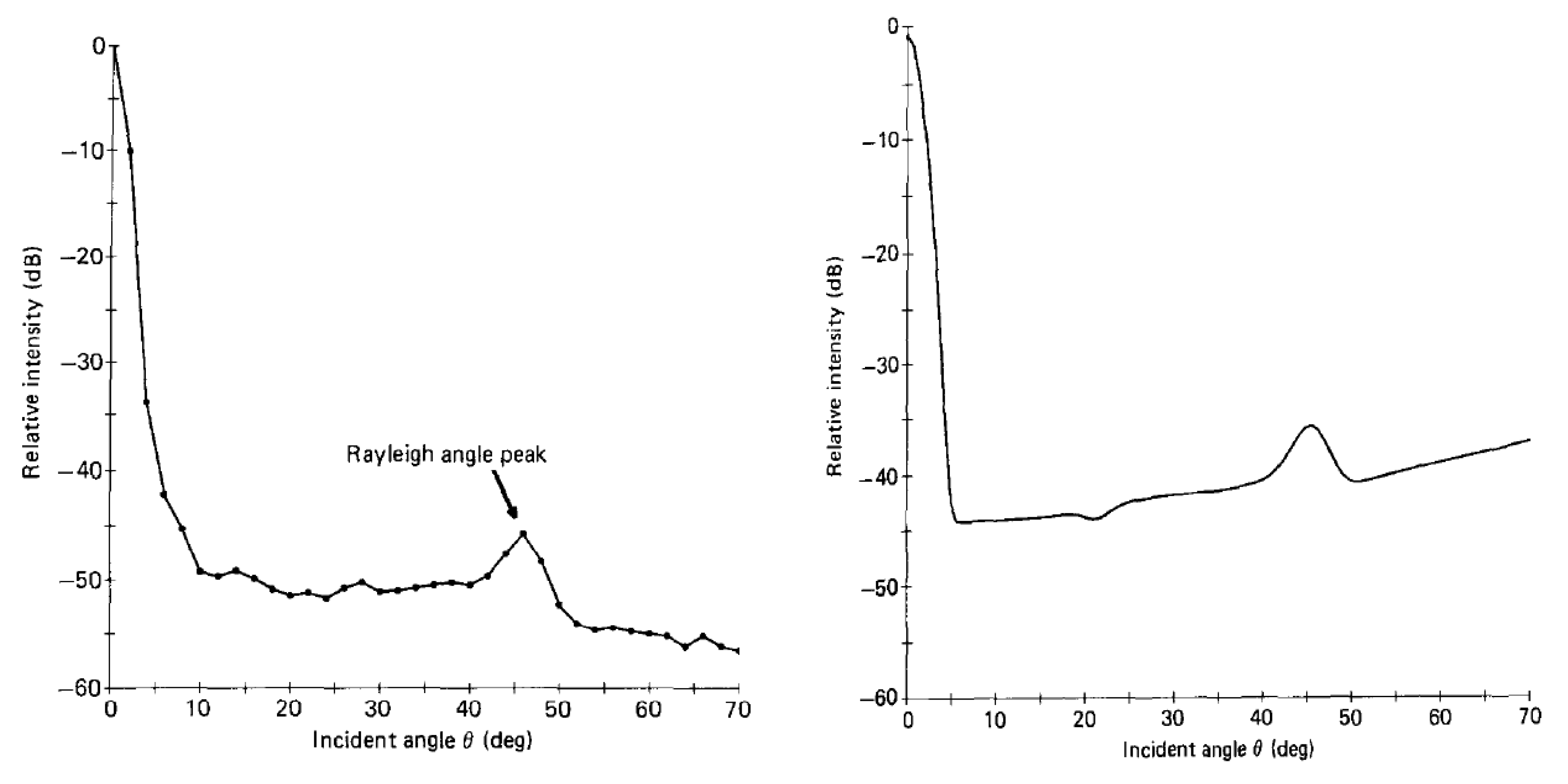
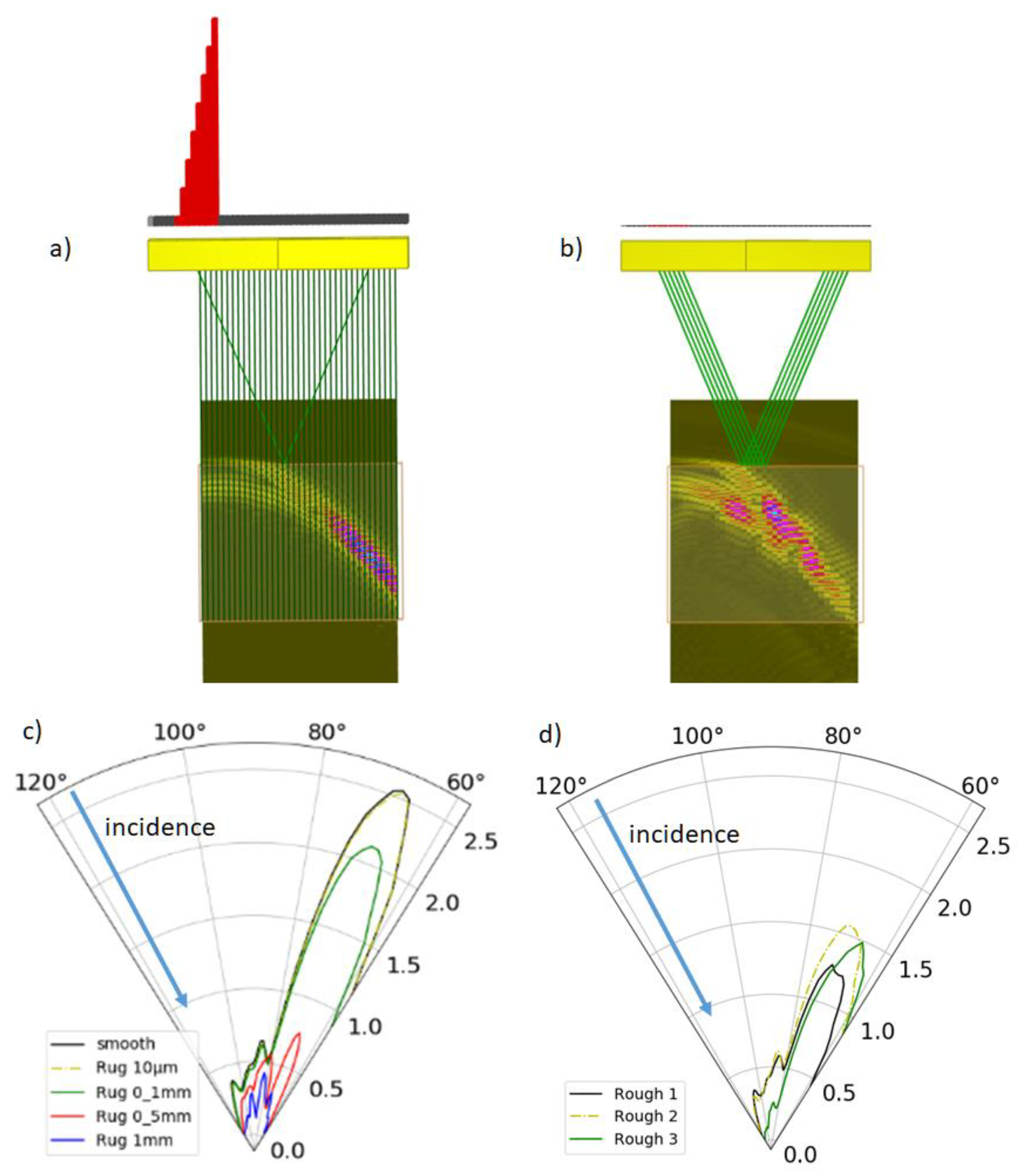
3.2.3. Elastic Targets and Applications

The Kirchhoff approximation models bulk waves, and does not take into account surface acoustics waves (SAW) as Rayleigh waves neither head waves. Head waves led to recent researches [70,86,87,88] and a modification [89] of the Kirchhoff approximation is henceforth proposed for head waves account. Head waves on irregular surfaces can also be modelled [90].

The Kirchhoff approximation for elastic rough targets is proposed by Ogilvy [13] and then revisited by Bjorno [91] and Dacol [92]. The Kirchhoff approximation validity have also been specifically considered in the particular cases of rigid and soft targets in a modeling study [93] of the reflected field including multiple scattering. One example of KA application to impedance surfaces [57] for non-destructive evaluation (NDE) is the modeling of ultrasonic telemetry of immersed targets [59,94].

We report here an application of KA simulation to impedance rough surfaces for NDE. Ultrasonic inspection of a planar steel component immersed in water (water path 25 mm) at frequency = 2 MHz (wavelength λ = 0.75 mm) is simulated with the Kirchhoff approximation for elastic rough entry surfaces of varying roughness using CIVA software inspection simulations tools [57,95,96]. A phased-array (represented in yellow in Figure 7a,b) is used to emit an incident beam directed at 117° with respect to the surface thanks an emission delay law (applied in red in Figure 7a to only some left elements) and all elements receives the scattered waves without delay law in the angular domain (118°, 58°).

In Figure 7a,b, the true B-scans (true-to-geometry imaging) are surperimposed to the specimen in color codes; they represent the echographic signal versus time for all elements in reception (corresponding to scattering angles in the angular domain (118°, 58°)). Figure 7c shows that increasing the roughness deteriorates the specular reflection echo and causes appearance of echoes at non-specular angles. Figure 7d shows that the scattering directivity patterns obtained for three different generated rough surfaces of the same statistical properties are slightly different.

A recent study [97] has compared the accuracy of KA and PT using a finite element (FE) model for fluid and elastic ocean bottoms. For a fluid bottom, KA is close to FE with maximal gap of 2 dB except for small grazing incident angles for which PT is more effective. PT behaves globally well except near specular observation direction notably for small grazing incident angles. For the elastic case, the disagreement between KA and FE increases to 5 dB and KA is inaccurate for incident angles less than the longitudinal critical angle: the interferences between transversal, longitudinal and surface waves are not taken into account in KA. The PT prediction is generally good, but another limitation appears in the elastic case for incident angles near the longitudinal critical one. However, we regret the provided validations are established only for a small roughness k $\sigma$= 0.6 favorable to PT.

3.2.4. Periodic Surfaces

As it will be discussed in the Section 5, Perspectives, it can also be useful to model scattering from periodic surfaces—such surfaces can notably appear in additive manufacturing parts or in oceans. For the case of periodic surfaces, one exact solution is the classical Rayleigh–Fourier method (RFM) [98]. Impinged by a plane wave, a periodic surface leads to Bragg scattering with a finite number of plane wave propagation angles in far field. A very recent study evaluates the validity of the Kirchhoff approximation (KA) for the scattering problem from a sinusoidal surface—mimicking the ocean one—with comparison to the RFM solution [99]. An asymptotic evaluation of the Kirchhoff integral which is consequently equivalent to geometrical acoustics [100] provides a ray theory which is also evaluated to better understand the Kirchhoff prediction. This notably shows that Kirchhoff has the advantage to exhibit a smooth behaviour near caustics generated by the sinusoidal surface contrary to geometrical acoustics. The KA validity is also studied versus the observation range (projected distance between the source and receiver points): for a short range, KA is very close to RFM. At moderate range, KA sometimes over-estimated the peak pressure due to interferences between several rays. For longer ranges, the KA disagreement increases strongly. This study [99] is very useful for better understanding the KA limitations due to multiple paths arrivals and grazing incidence/observation. Nevertheless, KA remains a very useful tool even for periodic surfaces when source and observations are not too far.

4. More Modern Approaches with Larger Domains of Validity

We have presented the two classical approximations: the perturbation theory (PT) and the Kirchhoff approximation (KA). In the view of main application to scattering from ocean, it is important to cite the two-scale roughness theories [101,102,103,104]. They consist in assuming that scattering can be considered as the combination of two phenomena: that produced by large facets and well approximated by KA and that due to small roughness and approximated by PT. One major inconvenient of this technique is that it requires to fix a wavenumber parameter [105] to separate the two scattering domains. The small slope approximation, described in the next section, is a much more convenient technique to link the classical approximations and it reduces to their results in some limiting cases.

In this section, some sound propagation models which have been notably devised for underwater acoustic applications and providing a better validity notably for grazing observation angles are studied. Underwater acoustic propagation depends on many factors. When sound propagates underwater the sound intensity decreases when increasing the propagation distance. Propagation loss is a quantitative measure of the reduction in sound intensity between two points, normally the sound source and a distant receiver. Modeling the acoustic reflection loss [106] at the rough ocean surface needs simulating forward scattering for incident grazing angles and is of interest for sonar especially for shallow oceans or oceans with a surface duct (sound waves trapped in a duct layer below the sea surface) [106]. Several models described hereafter (small slope approximation—SSA, and parabolic equation—PE) were notably designed to handle grazing angles. The integral equation (IE) method is also used as reference solution for validating SSA and comparing it to other approximations as KA and geometrical optics (GO).

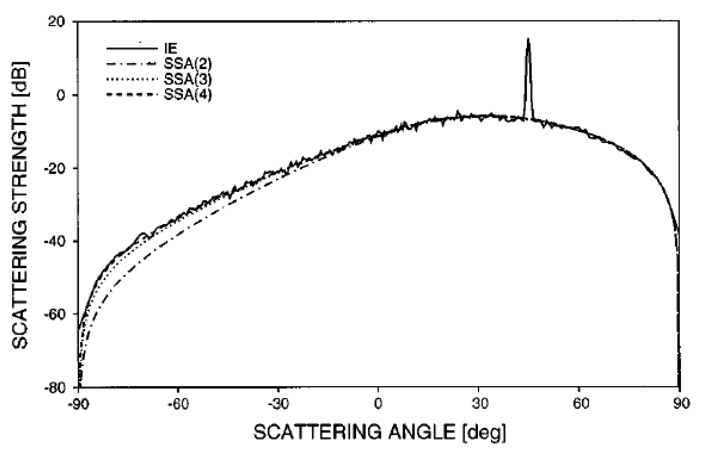
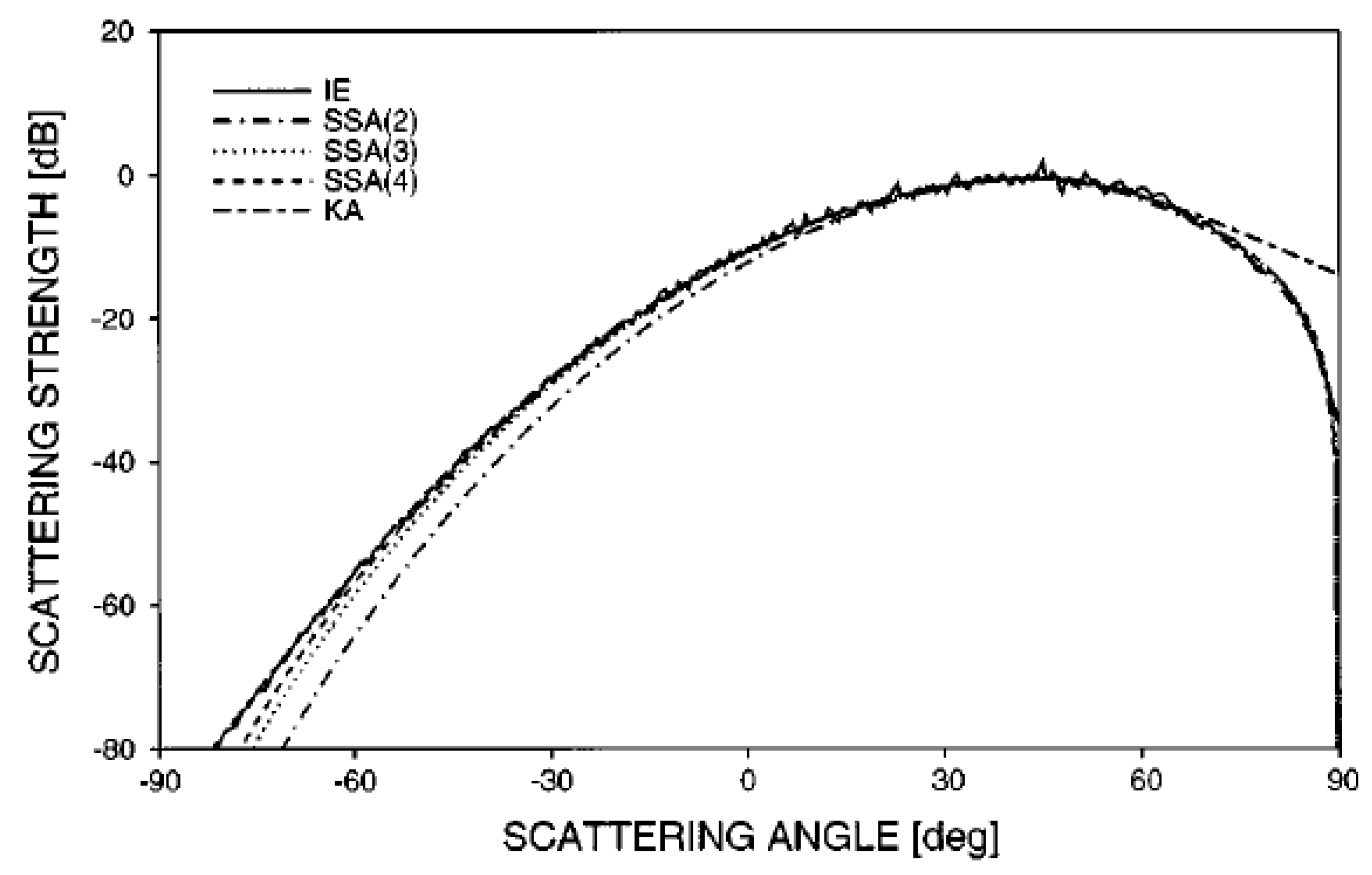
4.1. Small Slope Approximation (SSA)

The SSA technique was described first by Voronovich [107,108,109]. An alternative small slope approximation has originally been developed by Urusovskii and then studied by McDaniel (1994) [110]. All these methods attempt to exploit the assumed smallness of the surface slope without restricting the RMS surface height to wavelength ratio.

The SSA model from Voronovich has been investigated by Thorsos and Broschat [111,112]. SSA consists in introducing a roughness correction to the Helmholtz integral. This correction is expanded into a functional Taylor series in slope whose terms depend on the integral of the wave number spectrum of the surface height function. The approximation of each order of SSA is based on the approximations of previous orders. Owing to its principles SSA takes into account shadowing and diffraction.

Thorsos and Broschat showed that, at lowest order the small slope approximation of Urusovskii/McDaniel is limited to forward scattering [110] but that the lowest order term in Voronovich’s SSA was incorrect in McDaniel’s SSA.

SSA tends to the perturbation approximation for small k $\sigma$ (adimensional wave numbers in terms of RMS surface height $\sigma$). The second order SSA (SSA (2)) reduces to the Kirchhoff approximation (KA) at high frequencies, hence does not take into consideration the shadowing effects. The predictions of SSA(2), SSA(3), and SSA(4) are compared [112] with Monte Carlo integral equation (IE) calculations devised earlier by Thorsos [21], and with other approximations: the perturbation approximation, the Kirchhoff approximation (KA), and geometrical optics (GO). The scattering geometry is described in Figure 8.

SSA and IE scattering predictions are presented in Figure 9 for respective k $\sigma$ and kL 0.5 and 4.0, for 45° incident angle and RMS slope s = 0.177 ($s=\sqrt{2}\raisebox{1ex}{$\sigma $}\!\left/ \!\raisebox{-1ex}{$L$}\right.$ for Gaussian surface), and the RMS slope angle $\gamma ={\tan }^{-1}s$ is 10°. The contribution of specular reflection—leading to a peak in the IE prediction—has not been integrated in the SSA models.

In Figure 10, k $\sigma$ and kL have both been increased by a factor of three to 1.5 and 12.0, respectively. The increase in the surface roughness (resp. correlation length) causes disappearance of the specular peak (resp. decrease of the backscattered strength). A higher SSA order improves the prediction in backscattering.

According to Thorsos [21], the Kirchhoff approximation KA is accurate away from low grazing angles for rough surfaces smooth on the scale of a wavelength, assuming small surface slopes. For a Gaussian roughness spectrum, the KA is said to be generally accurate for kL >6, that is when $\raisebox{1ex}{$L$}\!\left/ \!\raisebox{-1ex}{$\lambda $}\right.>1$. We have seen in Section 3.2.2 the recent definition of a more precise criterion for the KA validity. In the following of this section the SSA and KA are thus considered for several examples with kL > 6.

In Thorsos’ previous Figure 3 [112], KA is valid away from grazing angles, whereas PT (not shown) is not. The SSA(2) result reduces to the KA result in the specular region; the third and fourth-order results do as well. KA behaves better than SSA for backscattering, but it is the contrary in the forward direction at grazing angles.

Finally, several cases have been examined beyond the region of validity of the fourth-order Perturbation Theory PT(4) and of KA. For example, in their Figure 6 [112] since k $\sigma$ = 1, PT(4) breaks down whereas KA is globally correct and SSA(4) the more realistic (Figure 11).

Other validations showed that the fourth-order SSA (SSA(4)) mimics some shadowing phenomena and the SSA results are globally accurate for all observation angles for incident angles up to 80°, but the validity decreases with the incident angle.

Another study [113] of the Bragg scattering from surface waves by a rough interface recently provided comparisons between the Kirchhoff approximation, the perturbation theory and the integral equation method; Kirchhoff leads to results relatively close to the integral equation method in the studied configurations (in forward and backscattering).

Voronovich (see Figure 1.1 in [20]) argued that SSA is valid for σ/L less than a constant value. According to him, KA and PT also require this condition but PT needs in addition a small kσ and KA a great kL.

SSA has also been developed for rough solid elastic interfaces [114]. Berman [115] showed that it provides an effective solution compared to Monte-Carlo integral equations simulations for grazing incident angles, whereas Kirchhoff leads to an overall important underestimation. SSA and first-order PT give rather good predictions and exhibit minima or peaks at the Rayleigh angle that can be exaggerated or discontinuities at critical angles which are not physical. The authors noted that Kirchhoff is rather smooth or does not have the valid behaviour for these particular angles: it is logical because the associated phenomena (Rayleigh or head waves) are not accounted on the simplified Kirchhoff theory (see also the perspectives section). We nevertheless notice that Kirchhoff yields an overall rather good prediction versus scattering angle despite some quantitative discrepancies. We also emphasise that one comparison shows an overestimation by first-order PT of the specular amplitude, which is a strong inconvenient for numerous applications as NDE.

SSA for layered fluid seafloors has only been studied recently. A study published this year [116] reviewed three different approximations. Jackson [117] has proposed an acoustic SSA method for rough water–sediment interfaces with a fluid layer of finite thickness overlying a semi-infinite fluid layer. A second method consists in using in acoustics the SSA developed for the general layered case in electromagnetics [118,119,120]. A third approach is developed in [116] by translating usual small-slope ansatz from k-space to coordinate space. It is then shown in [116] using different examples that the different approximations give different results in the case of strong internal reflections and also differ from Kirchhoff in specular direction. In an example with a mud layer overlying a harder basement, the first approximation differs strongly from the two others and consequently seems erroneous. Unfortunately, no numerical validation is provided to define the best ansatz.

4.2. Parabolic Equation (PE)

Acoustic losses at the rough ocean surface can be simulated utilizing a propagation code which can use as input an explicitly defined roughness profile. The PE (Parabolic equation [121,122,123]) model Ramsurf [124] is often used and enables to model shadowing from the surface roughness. Ramsurf is based on the split-step Padé method [121] (a pseudo-spectral numerical method for solving nonlinear partial differential equations).

Firstly, based on the rough ocean surface of Gaussian spectrum, the validity of Ramsurf acoustic propagation model has been studied [125] by comparison with measurements after an explosion at receivers located on the ocean bottom around 1000 m depth. The height for the sea surface is from 1.5 m to 2 m. Transmission loss curve under a smooth sea surface and that under the rough sea surface are simulated respectively by Ramsurf. The sea surface reflection loss caused by the surface roughness is about 4 to 6 dB. The transmission loss simulated by Ramsurf model is very close to the experimental one. Kirchhoff approximation (KA) and small slope approximation (SSA) abilities to simulate the reflection loss are also compared: SSA and Ramsurf match well for very small grazing angles (<6°) for which KA breaks down. We nevertheless notice that the gap between KA and Ramsurf becomes less than 3 dB above 6°: KA is thus inaccurate only in a very small region.

Another study [126] focuses on the modeling of underwater acoustical reflection from a wind-roughened ocean surface and compares the surface loss between KA, a small-slope model SSA(2) and a stochastic modeling using Ramsurf. SSA(2) matches well with Ramsurf for the entire range of frequency and wind speed combinations studied (1.5–9 kHz, 5–12.5 m/s) and for sound incidence grazing angles from 1 to 11°. KA can be used effectively from an angle about 2.5 to 7°.

An extension of the parabolic equation method to deal with forward scattering has recently been proposed for both Dirichlet and Neumann boundary conditions [127] but future works are needed to make the connection between forward and backward 3D scattering and treat other boundary conditions.

5. Summary, Discussion and Perspectives

A review of acoustic wave scattering from rough surfaces has been done. Several analytical models proposed in the literature have been described in more detail as well as their validity. We are also focused in specific acoustic applications as scattering from ocean, non-destruction evaluation, medical sciences.

Two classical approximations have been early devised: the perturbation theory and the Kirchhoff approximation.

The perturbation theory (PT) consists in expressing the scattered field in an expansion series using as small parameter the roughness height. This method leads to a major inconvenient: it is valid for low roughness when compared to acoustic wavelength (at first order for small kσ < 2 to 4 depending on kL value, σ, L and k being respectively the rms roughness height, the correlation height and the wave number). Existing validations also showed that PT is rather accurate far from the specular direction. Consequently, it appears possibly more restrictive than the Kirchhoff method for numerous applications notably non-destruction evaluation (NDE) which usually employs inspection in specular direction.

The Kirchhoff approximation (KA) leads to a simple analytical expression; it is a relatively powerful and inexpensive approximation in terms of calculations and easily extended to impedance rough surfaces. One important fact is that KA is the most used method in NDE for rough surfaces: its implementation of the rough structure echo consists in simply modifying that of the smooth surface; the “rough” KA algorithm can thus simply mesh the smooth mean surface (surface without roughness) in small surface elements and then modify the contribution of each mesh point by including some local geometrical parameters of the rough surface.

KA has the advantage of handling surfaces of roughness smaller than a constant depending on the wavelength and on the correlation length with a relatively satisfying validity except at the vicinity of grazing observation and critical angles. Indeed we have connected and merged recent studies of the KA validity and conclude that for many applications using rather near specular observation and nongrazing incident angles, two criteria can be used for KA validity: σ²/L ≤ Cλp (C and λp being a constant value and the wavelength) and kL >1 or 2. If we do not want to limit the KA validity to near specular observation, the previous criteria are likely to be a little more restrictive to reach the KA validity for incidence and scattering angles over the range from −80° to 80°(kL > π is for instance needed)

It is well admitted that KA validity for application to rough surfaces decreases for grazing angles and the region of inaccuracy in terms of scattering angles is much more important for a fluid/solid interface. One has to pay attention at the KA validity in the vicinity of particular angles (Rayleigh and critical ones). In NDE inspections, these angles are often avoided by the inspector; nevertheless it may be possible to meet them in some geometrical configurations. Improving KA or analytical approximations to better take into account head waves occurring at critical angles is an important challenge already for planar surfaces [128]. Modeling head waves on irregular surfaces is even more complicated and seems intractable using analytical methods [90,129]. Finite elements methods [130] can be useful to model both the head waves generated at critical angles, the bulk waves radiated near the surface and their possible interferences [90,129].

For planar surfaces, some smoothing modifications of KA can be proposed [69] in the vicinity of critical angles for better validity, but they do not simulate head waves. A modification of KA using an alternative integral formula for the Kirchhoff integral has just been developed [89], and it could be extended to scattering from a rough surface. Nevertheless, this perspective has to be tested and validated, since such a model will generate head waves as if they have been created on successive local non-finite tangential plane.

PT and KA are usually seen as complementary, PT being valid for small roughness scales and Kirchhoff for large scales. Several other approximations have been developed in the view of handling the inconveniences of the classical methods (PT and KA) and enlarge the simulation validity. Some of them (phase perturbation theory, two-scales models) found some applications in electromagnetism. A recent study [131] has just began in order to try to improve the two-scale models. We are not convinced that improving these models is the best perspective because they inherently own a certain complexity and there are probably better candidates (evoked in the following) in simulation methods.

The small slope approximation (SSA) is a model based on an integral field equation; it is more efficient than Kirchhoff for grazing angles but is only valid for small surface slopes. Indeed, the SSA is of great importance in ocean applications for modeling scattering from ocean surfaces on which the incidence is generally near from grazing: in such a configuration the SSA accuracy is well established. One main future challenge is to extend this approximation to layered fluid seafloors. In a study published this year [116], different approximations are proposed but they give different results in the case of strong internal reflections and also differ from Kirchhoff in specular direction. Numerical validations are clearly needed to try to find the best approximation among them; another problem is that only one extended from electromagnetism [118] can deal with multiple layers.

The parabolic equation describes all physical effects including shadowing, but this method needs a complex and heavy numerical technique to solve the parabolic equation. The parabolic equation method has recently been extended to forward scattering, but numerous efforts should be necessary in the future to build a more robust model applicable for both forward and backward 3D scattering. Such a strategy can be seen complex when compared to other methods as fully numerical ones which are generic for all scattering directions.

There is also recent progress in methods based on the integral equation; for instance the new development described in [132] leads to impressive results, notably for grazing angles; but the calculation time is still for the moment a limitation by comparison with simpler methods, if we are rather interested in near normal incidence.

Numerical methods are obviously the main rivals of the existing analytical models. For numerical techniques, obtaining 3D simulations with a reasonable computation time remains a challenge. In a very recent study, the boundary element method has been adapted [133] to reduce the 3D calculation time; the proposed adaptation is validated by using approximated models (KA and PT) showing that the classical approximations are also useful for validation purposes.

In the field of NDE, one major future challenge is to model scattering from roughness in components fabricated by additive manufacturing (AM). The fatigue life of AM specimens is very influenced by their surface topography [134]. AM processes for metallic parts are notably the selective laser melting (SLM), selective electron beam melting (SEBM), laser metal deposition (LMD) and also wire arc additive manufacturing (WAAM [135]). The corresponding roughness value of each process is discussed in [136,137]: it is 4–11 µm Ra for SLM, 15–35 µm Ra for SEBM, 10 µm Ra and 200 µm Ra for LMD, and can be very important for WAAM. Note that models are searched for the prediction of surface roughness (see a list of studies in the introduction of [138]), the optimization of process parameters as well as the roughness minimization (as in [138]) for manufacturing using WAAM and milling.

In AM processes there a lot of phenomena causing roughness [139,140], notably the sticking of nonmelted or partially melted particles on the surfaces and the formation of menisci. The latter phenomenon is more pronounced for the WAAM process (see Figure 12, below).

The balling effect (Figure 13) is a detrimental phenomenon that may result in breaking up the liquid scan track during SLM and produce particles in spherical shapes.

The rough surface of AM parts can thus exhibit a kind of periodicity and elementary egg-shaped irregularities [142]. Finite element models [143] are likely to be the best solution to both model the bulk macrostructure of such components and their surface roughness—such models have been recently used to model scattering in virtual simulated microstructures of polycrystalline materials either with equiaxed grains [144,145,146] or transverse isotropic as in austenitic welds [147]. The increasing power brought by the spectral finite elements (SEM) method is noticeable [148,149,150] in terms of calculation time and could be very useful for roughness with complex shape irregularities; SEM has recently been used for modeling ultrasonic propagation in granular materials, such as concrete [151].

In another domain, a FEM model has just been employed to model the ultrasonic response of bone–dental implant interfaces [5,152] whose irregularities can generate multiple scattering. Such a numerical method also presents the advantage of being easily adaptable in the future, for instance to treat non-linear effects at the contact interface. All the previous examples show the increase of applications for numerical methods.

References

1. Romanova, A.V.; Horoshenkov, K.V.; Krynkin, A. Dynamically Rough Boundary Scattering Effect on a Propagating Continuous Acoustical Wave in a Circular Pipe with Flow. Sensors 2018, 18, 1098. [Google Scholar] [CrossRef] [PubMed] [Green Version]
2. Wang, Z.; Cui, X.; Ma, H.; Kang, Y.; Deng, Z. Effect of Surface Roughness on Ultrasonic Testing of Back-Surface Micro-Cracks. Appl. Sci. 2018, 8, 1233. [Google Scholar] [CrossRef] [Green Version]
3. Dingler, J.R.; Boylls, J.C.; Lowe, R.L. A high-frequency sonar for profiling small-scale subaqueous bedforms. Mar. Geol. 1977, 24, 279–288. [Google Scholar] [CrossRef]
4. Niu, L.; Qian, M.; Yang, W.; Meng, L.; Xiao, Y.; Wong, K.K.L.; Abbott, D.; Liu, X.; Zheng, H. Surface Roughness Detection of Arteries via Texture Analysis of Ultrasound Images for Early Diagnosis of Atherosclerosis. PLoS ONE 2013, 8, e76880. [Google Scholar] [CrossRef] [PubMed] [Green Version]
5. Hériveaux, Y.; Nguyen, V.-H.; Biwa, S.; Haïat, G. Analytical modeling of the interaction of an ultrasonic wave with a rough bone-implant interface. Ultrasonics 2020, 108. [Google Scholar] [CrossRef]
6. Ogilvy, J.A. Model for the ultrasonic inspection of rough defects. Ultrasonics 1989, 28, 69–79. [Google Scholar] [CrossRef]
7. Ogilvy, J.A. Theoretical comparison of ultrasonic signal amplitudes from smooth and rough defects. NDT Int. 1986, 19, 371–385. [Google Scholar] [CrossRef]
8. Ogilvy, J.A.; Culverwell, I.D. Elastic model for simulating ultrasonic inspection of smooth and rough defects. Ultrasonics 1991, 29, 490–496. [Google Scholar] [CrossRef]
9. Nagy, P.B.; Adler, L. Surface roughness induced attenuation of reflected and transmitted ultrasonic waves. J. Acoust. Soc. Am. 1987, 82, 193–197. [Google Scholar] [CrossRef]
10. Nagy, P.B.; Rose, J.H. Surface roughness and the ultrasonic detection of subsurface scatterers. J. Appl. Phys. 1993, 73, 566–580. [Google Scholar] [CrossRef]
11. Nagy, P.B.; Adler, L.; Rose, J.H. Effects of Acoustic Scattering at Rough Surfaces on the Sensitivity of Ultrasonic Inspection. In Review of Progress in Quantitative Nondestructive Evaluation; Springer: Boston, MA, USA, 1993; pp. 1775–1782. ISBN 978-1-4613-6233-3. [Google Scholar]
12. Bilgen, M. Effects of randomly rough surfaces on ultrasonic inspection. Retrosp. Theses Diss. 1993. [Google Scholar] [CrossRef]
13. Ogilvy, J.A. Theory of Wave Scattering From Random Rough Surfaces; Taylor & Francis: Abingdon, UK, 1991; ISBN 978-0-7503-0063-6. [Google Scholar]
14. Elfouhaily, T.M.; Guérin, C.-A. A critical survey of approximate scattering wave theories from random rough surfaces. Waves Random Media 2004, 14, R1–R40. [Google Scholar] [CrossRef]
15. Ishimaru, A. Wave-Propagation and Scattering in Random-Media and Rough Surfaces. Proc. IEEE 1991, 79, 1359–1366. [Google Scholar] [CrossRef] [Green Version]
16. Ticconi, F.; Pulvirenti, L.; Pierdicca, N. Models for Scattering from Rough Surfaces. Electromagn. Waves 2011. [Google Scholar] [CrossRef] [Green Version]
17. Hermansson, P.; Forssell, G. A Review of Models for Scattering from Rough Surfaces. Available online: https://scholar.google.com/scholar?cluster=9344336395593944459&hl=fr&as_sdt=0,5&sciodt=0,5 (accessed on 25 March 2020).
18. Ogilvy, J.A. Wave scattering from rough surfaces. Rep. Prog. Phys. 1987, 50, 1553–1608. [Google Scholar] [CrossRef]
19. Brekhovskikh, L.M.; Lysanov, Y.P. Fundamentals of Ocean Acoustics; Springer Science & Business Media: Berlin/Heidelberg, Germany, 2013; ISBN 978-3-662-07328-5. [Google Scholar]
20. Voronovich, A.G. Wave Scattering from Rough Surfaces; Springer Science & Business Media: Berlin/Heidelberg, Germany, 2013; ISBN 978-3-642-59936-1. [Google Scholar]
21. Thorsos, E.I. The validity of the Kirchhoff approximation for rough surface scattering using a Gaussian roughness spectrum. J. Acoust. Soc. Am. 1988, 83, 78–92. [Google Scholar] [CrossRef] [Green Version]
22. Khenchaf, A.; Daout, F.; Saillard, J. The two-scale model for random rough surface scattering. In Proceedings of the OCEANS 96 MTS/IEEE Conference Proceedings. The Coastal Ocean-Prospects for the 21st Century, Fort Lauderdale, FL, USA, 23–26 September 1996; IEEE: Piscataway, NY, USA, 1996; Volume 2, pp. 887–891. [Google Scholar]
23. Nayak, P.R. Random Process Model of Rough Surfaces. J. Lubr. Technol. 1971, 93, 398–407. [Google Scholar] [CrossRef]
24. Johnson, K.L.; Johnson, K.L. Contact Mechanics; Cambridge University Press: Cambridge, UK, 1987; ISBN 978-0-521-34796-9. [Google Scholar]
25. Adler, R.J.; Firmin, D.; Kendall, D.G. A non-gaussian model for random surfaces. Philos. Trans. R. Soc. Lond. Ser. Math. Phys. Sci. 1981, 303, 433–462. [Google Scholar] [CrossRef]
26. Pérez-Ràfols, F.; Almqvist, A. Generating randomly rough surfaces with given height probability distribution and power spectrum. Tribol. Int. 2019, 131, 591–604. [Google Scholar] [CrossRef]
27. Ogilvy, J.A. Computer simulation of acoustic wave scattering from rough surfaces. J. Phys. Appl. Phys. 1988, 21, 260–277. [Google Scholar] [CrossRef]
28. Civa Software Website. Available online: http://www.extende.com/ (accessed on 20 November 2020).
29. Mahaut, S.; Chatillon, S.; Darmon, M.; Leymarie, N.; Raillon, R.; Calmon, P. An overview of ultrasonic beam propagation and flaw scattering models in the civa software. AIP Conf. Proc. 2010, 1211, 2133–2140. [Google Scholar] [CrossRef]
30. Toullelan, G.; Raillon, R.; Chatillon, S.; Dorval, V.; Darmon, M.; Lonné, S. Results of the 2015 UT Modeling Benchmark Obtained with Models Implemented in Civa. AIP Conf. Proc. 2016. [Google Scholar] [CrossRef] [Green Version]
31. Raillon-Picot, R.; Toullelan, G.; Darmon, M.; Calmon, P.; Lonné, S. Validation of CIVA ultrasonic simulation in canonical configurations. In Proceedings of the World Conference of Non Destructive Testing (WCNDT) 2012, Durban, South Africa, 16–20 April 2012. [Google Scholar]
32. Raillon, R.; Bey, S.; Dubois, A.; Mahaut, S.; Darmon, M. Results of the 2010 ut modeling benchmark obtained with civa: Responses of backwall and surface breaking notches. AIP Conf. Proc. 2011, 1335, 1777–1784. [Google Scholar] [CrossRef]
33. Raillon, R.; Bey, S.; Dubois, A.; Mahaut, S.; Darmon, M. Results of the 2009 ut modeling benchmark obtained with civa: Responses of notches, side-drilled holes and flat-bottom holes of various sizes. AIP Conf. Proc. 2010, 1211, 2157–2164. [Google Scholar] [CrossRef]
34. Gilbert, F.; Knopoff, L. Seismic scattering from topographic irregularities. J. Geophys. Res. 1896–1977 1960, 65, 3437–3444. [Google Scholar] [CrossRef]
35. Bass, F.G.; Fuks, I.M. Wave Scattering from Statistically Rough Surfaces; Pergamon Press: Oxford, UK, 1973. [Google Scholar]
36. Blakemore, M. Blakemore Scattering of acoustic waves by the rough surface of an elastic solid. Ultrasonics 1993, 31, 161–174. [Google Scholar] [CrossRef]
37. De Billy, M.; Quentin, G. Backscattering of acoustic waves by randomly rough surfaces of elastic solids immersed in water. J. Acoust. Soc. Am. 1982, 72, 591–601. [Google Scholar] [CrossRef]
38. Kuperman, W.A.; Schmidt, H. Self-consistent perturbation approach to rough surface scattering in stratified elastic media. J. Acoust. Soc. Am. 1989, 86, 1511–1522. [Google Scholar] [CrossRef]
39. Thorsos, E.I.; Jackson, D.R.; Williams, K.L. Modeling of subcritical penetration into sediments due to interface roughness. J. Acoust. Soc. Am. 1999, 107, 263–277. [Google Scholar] [CrossRef]
40. Jackson, D.R.; Ivakin, A.N. Scattering from elastic sea beds: First-order theory. J. Acoust. Soc. Am. 1998, 103, 336–345. [Google Scholar] [CrossRef] [Green Version]
41. Liu, J.Y.; Huang, C.F.; Hsueh, P.C. Acoustic plane-wave scattering from a rough surface over a random fluid medium. Ocean Eng. 2002, 29, 915–930. [Google Scholar] [CrossRef]
42. Liu, J.Y.; Tsai, S.H.; Wang, C.C.; Chu, C.R. Acoustic wave reflection from a rough seabed with a continuously varying sediment layer overlying an elastic basement. J. Sound Vib. 2004, 275, 739–755. [Google Scholar] [CrossRef]
43. Tang, D.; Jackson, D. A time-domain model for seafloor scattering. J. Acoust. Soc. Am. 2017, 142, 2968–2978. [Google Scholar] [CrossRef] [PubMed]
44. Bjorno, L. Scattering of plane acoustic waves at elastic particles with rough surfaces. J. Acoust. Soc. Am. 2015, 137, 2439. [Google Scholar] [CrossRef]
45. Neighbors, T.; Bradley, D. Applied Underwater Acoustics: Leif Bjørnø; Elsevier: Amsterdam, The Netherlands, 2017; ISBN 978-0-12-811247-2. [Google Scholar]
46. Faran, J.J. Sound Scattering by Solid Cylinders and Spheres. J. Acoust. Soc. Am. 1951, 23, 405–418. [Google Scholar] [CrossRef]
47. Flax, L.; Dragonette, L.R.; Überall, H. Theory of elastic resonance excitation by sound scattering. J. Acoust. Soc. Am. 1978, 63, 723–731. [Google Scholar] [CrossRef]
48. Masood, F.; Amin, U.; Fiaz, M.A.; Ashraf, M.A. On relating the perturbation theory and random cylinder generation to study scattered field. Phys. Commun. 2020, 39, 101003. [Google Scholar] [CrossRef]
49. Winebrenner, D.; Ishimaru, A. Investigation of a surface field phase perturbation technique for scattering from rough surfaces. Radio Sci. 1985, 20, 161–170. [Google Scholar] [CrossRef]
50. Winebrenner, D.P.; Ishimaru, A. Application of the phase-perturbation technique to randomly rough surfaces. JOSA A 1985, 2, 2285–2294. [Google Scholar] [CrossRef]
51. Broschat, S.L.; Tsang, L.; Ishimaru, A.; Thorsos, E.I. A Numerical Comparison of the Phase Perturbation Technique with the Classical Field Perturbation and Kirchhoff Approximations for Random Rough Surface Scattering. J. Electromagn. Waves Appl. 1988, 2, 85–102. [Google Scholar] [CrossRef]
52. Broschat, S.L.; Thorsos, E.I.; Ishimaru, A. The Phase Perturbation Technique vs. an Exact Numerical Method for Random Rough Surface Scattering. J. Electromagn. Waves Appl. 2012. [Google Scholar] [CrossRef]
53. Zhang, X.D.; Wu, Z.S.; Wu, C.K. A phase-perturbation technique for light scattering from randomly dielectric rough surfaces. Chin. Phys. Lett. 1997, 14, 32–35. [Google Scholar]
54. Meecham, W.C. On the use of the Kirchhoff approximation for the solution of reflection problems. Eng. Res. Inst. Dep. Phys. Mich. Univ. 1955, 5, 323–334. [Google Scholar] [CrossRef]
55. Bouche, D.; Molinet, F.; Mittra, R. Asymptotic Methods in Electromagnetics; Springer: Berlin/Heidelberg, Germany, 1997. [Google Scholar]
56. Chungang, J.; Lixin, G.; Pengju, Y. Time-Domain Physical Optics Method for the Analysis of Wide-Band EM Scattering from Two-Dimensional Conducting Rough Surface. Available online: https://www.hindawi.com/journals/ijap/2013/584260/ (accessed on 21 September 2020).
57. Dorval, V.; Chatillon, S.; Lu, B.; Darmon, M.; Mahaut, S. A general Kirchhoff approximation for echo simulation in ultrasonic NDT. AIP Conf. Proc. 2012, 1430, 193–200. [Google Scholar] [CrossRef] [Green Version]
58. Darmon, M.; Leymarie, N.; Chatillon, S.; Mahaut, S. Modelling of Scattering of Ultrasounds by Flaws for NDT. In Ultrasonic Wave Propagation in Non Homogeneous Media; Springer: Berlin/Heidelberg, Germany, 2009; Volume 128, pp. 61–71. [Google Scholar]
59. Lu, B.; Darmon, M.; Potel, C.; Zernov, V. Models Comparison for the scattering of an acoustic wave on immersed targets. J. Phys. Conf. Ser. 2012, 353, 012009. [Google Scholar] [CrossRef] [Green Version]
60. Keller, J.B. Geometrical theory of diffraction. J. Opt. Soc. Am. 1962, 52, 116–130. [Google Scholar] [CrossRef]
61. Darmon, M.; Chatillon, S.; Mahaut, S.; Fradkin, L.; Gautesen, A. Simulation of disoriented flaws in a TOFD technique configuration using GTD approach. In Proceedings of the 34th Annual Review of Progress in Quantitative Nondestructive Evaluation, Chicago, IL, USA, 20–25 July 2008; Volume 975, pp. 155–162. [Google Scholar]
62. Chaffai, S.; Darmon, M.; Mahaut, S.; Menand, R. Simulations tools for TOFD inspection in Civa software. In Proceedings of the ICNDE 2007, Istanbul, Turkey, 15–20 April 2007. [Google Scholar]
63. Darmon, M.; Ferrand, A.; Dorval, V.; Chatillon, S.; Lonné, S. Recent Modelling Advances for Ultrasonic TOFD Inspections. In AIP Conference Proceedings; AIP Publishing: College Park, MD, USA, 2015; Volume 1650, pp. 1757–1765. [Google Scholar]
64. Chehade, S.; Kamta Djakou, A.; Darmon, M.; Lebeau, G. The spectral functions method for acoustic wave diffraction by a stress-free wedge: Theory and validation. J. Comput. Phys. 2019, 377, 200–218. [Google Scholar] [CrossRef]
65. Chehade, S.; Darmon, M.; Lebeau, G. 2D elastic plane-wave diffraction by a stress-free wedge of arbitrary angle. J. Comput. Phys. 2019, 394, 532. [Google Scholar] [CrossRef]
66. Ufimtsev, P.Y. Fundamentals of the Physical Theory of Diffraction; John Wiley & Sons: Hoboken, NJ, USA, 2007. [Google Scholar]
67. Lü, B.; Darmon, M.; Fradkin, L.; Potel, C. Numerical comparison of acoustic wedge models, with application to ultrasonic telemetry. Ultrasonics 2016, 65, 5–9. [Google Scholar] [CrossRef] [Green Version]
68. Zernov, V.; Fradkin, L.; Darmon, M. A refinement of the Kirchhoff approximation to the scattered elastic fields. Ultrasonics 2012, 52, 830–835. [Google Scholar] [CrossRef]
69. Darmon, M.; Dorval, V.; Kamta Djakou, A.; Fradkin, L.; Chatillon, S. A system model for ultrasonic NDT based on the Physical Theory of Diffraction (PTD). Ultrasonics 2016, 64, 115–127. [Google Scholar] [CrossRef] [PubMed] [Green Version]
70. Fradkin, L.J.; Darmon, M.; Chatillon, S.; Calmon, P. A semi-numerical model for near-critical angle scattering. J. Acoust. Soc. Am. 2016, 139, 141–150. [Google Scholar] [CrossRef] [PubMed] [Green Version]
71. Djakou, A.K.; Darmon, M.; Fradkin, L.; Potel, C. The Uniform geometrical Theory of Diffraction for elastodynamics: Plane wave scattering from a half-plane. J. Acoust. Soc. Am. 2015, 138, 3272–3281. [Google Scholar] [CrossRef] [PubMed]
72. Eckart, C. The Scattering of Sound from the Sea Surface. J. Acoust. Soc. Am. 1953, 25, 566–570. [Google Scholar] [CrossRef]
73. Imbert, C. Visualisation Ultrasonore Rapide Sous Sodium Application Aux Reacteurs a Neutrons Rapides; INSA de Lyon: Villeurbanne, France, 1997. [Google Scholar]
74. Wagner, R.J. Shadowing of Randomly Rough Surfaces. J. Acoust. Soc. Am. 1967, 41, 138–147. [Google Scholar] [CrossRef]
75. Zverev, V.A.; Slavinskii, M.M. A method for calculating the acoustic field near a rough surface. Acoust. Phys. 1997, 43, 56–60. [Google Scholar]
76. Chapman, D.M.F. An improved Kirchhoff formula for reflection loss at a rough ocean surface at low grazing angles. J. Acoust. Soc. Am. 1983, 73, 520–527. [Google Scholar] [CrossRef]
77. Shi, F.; Choi, W.; Lowe, M.J.S.; Skelton, E.A.; Craster, R.V. The validity of Kirchhoff theory for scattering of elastic waves from rough surfaces. Proc. R. Soc. Math. Phys. Eng. Sci. 2015, 471, 20140977. [Google Scholar] [CrossRef]
78. Haslinger, S.G. Elastic shear wave scattering by randomly rough surfaces. J. Mech. Phys. Solids 2020, 137, 103852. [Google Scholar] [CrossRef]
79. Haslinger, S.G.; Lowe, M.J.S.; Huthwaite, P.; Craster, R.V.; Shi, F. Appraising Kirchhoff approximation theory for the scattering of elastic shear waves by randomly rough defects. J. Sound Vib. 2019, 460, 114872. [Google Scholar] [CrossRef]
80. Opsal, J.L.; Visscher, W.M. Theory of elastic wave scattering: Applications of the method of optimal truncation. J. Appl. Phys. 1985, 58, 1102–1115. [Google Scholar] [CrossRef]
81. Becache, E.; Joly, P.; Tsogka, C. An analysis of new mixed finite elements for the approximation of wave propagation problems. SIAM J. Numer. Anal. 2000, 37, 1053–1084. [Google Scholar] [CrossRef] [Green Version]
82. Becache, E.; Joly, P.; Tsogka, C. Application of the fictitious domain method to 2D linear elastodynamic problems. J. Comput. Acoust. 2001, 9, 1175–1202. [Google Scholar]
83. Huang, R.; Schmerr, L.W., Jr.; Sedov, A.; Gray, T.A. Kirchhoff approximation revisited—Some new results for scattering in isotropic and anisotropic elastic solids. Res. Nondestruct. Eval. 2006, 17, 137–160. [Google Scholar] [CrossRef]
84. Darmon, M. Validity of the Kirchhoff Approximation for Small Flaws; CEA/DISC/LSMA: Saclay, France, 2014. [Google Scholar]
85. Zhang, J.; Drinkwater, B.W.; Wilcox, P.D. Longitudinal Wave Scattering from Rough Crack-Like Defects. IEEE Trans. Ultrason. Ferroelectr. Freq. Control 2011, 58, 2171–2180. [Google Scholar] [CrossRef]
86. Zernov, V.; Fradkin, L.; Gautesen, A.; Darmon, M.; Calmon, P. Wedge diffraction of a critically incident Gaussian beam. Wave Motion 2013, 50, 708–722. [Google Scholar] [CrossRef]
87. Zernov, V.; Gautesen, A.; Fradkin, L.J.; Darmon, M. Aspects of diffraction of a creeping wave by a back-wall crack. J. Phys. Conf. Ser. 2012, 353, 012017. [Google Scholar] [CrossRef] [Green Version]
88. Mahaut, S.; Huet, G.; Darmon, M. Modeling of Corner Echo in UT Inspection Combining Bulk and Head Waves Effect. In Proceedings of the 35th Annual Review of Progress in Quantitative Nondestructive Evaluation, 35th Annual Review of Progress in Quantitative Nondestructive Evaluation, Chicago, IL, USA, 20–25 July 2008; Volume 1096, pp. 73–80. [Google Scholar]
89. Fradkin, L.J.; Djakou, A.K.; Prior, C.; Darmon, M.; Chatillon, S.; Calmon, P.-F. The Alternative Kirchhoff Approximation in Elastodynamics with Applications in Ultrasonic Nondestructive Testing. ANZIAM J. 2020, 1–17. [Google Scholar] [CrossRef]
90. Ferrand, A.; Darmon, M.; Chatillon, S.; Deschamps, M. Modeling of ray paths of head waves on irregular interfaces in TOFD inspection for NDE. Ultrasonics 2014, 54, 1851–1860. [Google Scholar] [CrossRef] [Green Version]
91. Bjorno, L.; Sun, S. Use of the Kirchhoff Approximation in Scattering from Elastic, Rough Surfaces. Acoust. Phys. 1995, 41, 637–648. [Google Scholar]
92. Dacol, D.K. The Kirchhoff approximation for acoustic scattering from a rough fluid–elastic solid interface. J. Acoust. Soc. Am. 1998, 88, 978. [Google Scholar] [CrossRef]
93. Gavrilov, A.L.; Dunin, S.Z.; Maskomov, G.A. Scattering of scalar fields by hard and soft rough surfaces. Angular distribution of intensity. Akust. Zhurnal 1992, 38, 861–873. [Google Scholar]
94. Ploix, M.-A.; Kauffmann, P.; Chaix, J.-F.; Lillamand, I.; Baqué, F.; Corneloup, G. Acoustical properties of an immersed corner-cube retroreflector alone and behind screen for ultrasonic telemetry applications. Ultrasonics 2020, 106. [Google Scholar] [CrossRef] [PubMed]
95. Darmon, M.; Chatillon, S. Main Features of a Complete Ultrasonic Measurement Model: Formal Aspects of Modeling of Both Transducers Radiation and Ultrasonic Flaws Responses. Open J. Acoust. 2013, 3, 36873. [Google Scholar] [CrossRef] [Green Version]
96. Mahaut, S.; Darmon, M.; Chatillon, S.; Jenson, F.; Calmon, P. Recent advances and current trends of ultrasonic modelling in CIVA. Insight 2009, 51, 78–81. [Google Scholar] [CrossRef]
97. Isakson, M.J.; Chotiros, N.P. Finite Element Modeling of Acoustic Scattering from Fluid and Elastic Rough Interfaces. IEEE J. Ocean. Eng. 2015, 40, 475–484. [Google Scholar] [CrossRef]
98. Botten, L.C.; Cadilhac, M.; Derrick, G.H.; Maystre, D.; McPhedran, R.C.; Nevière, M.; Vincent, P. Electromagnetic Theory of Gratings; Springer Science & Business Media: Berlin/Heidelberg, Germany, 2013; Volume 22. [Google Scholar]
99. Richards, E.L.; Song, H.C.; Hodgkiss, W.S. Acoustic scattering comparison of Kirchhoff approximation to Rayleigh-Fourier method for sinusoidal surface waves at low grazing angles. J. Acoust. Soc. Am. 2018, 144, 1269–1278. [Google Scholar] [CrossRef]
100. Williams, K.L.; Stroud, J.S.; Marston, P.L. High-frequency forward scattering from Gaussian spectrum, pressure release, corrugated surfaces. I. Catastrophe theory modeling. J. Acoust. Soc. Am. 1994, 96, 1687–1702. [Google Scholar] [CrossRef]
101. Kur’yanov, B.F. The scattering of sound at a rough surface with two types of irregularity. Sov. Phys. Acoust. 1963, 8, 252–257. [Google Scholar]
102. McDaniel, S.T.; Gorman, A.D. An examination of the composite-roughness scattering model. J. Acoust. Soc. Am. 1983, 73, 1476–1486. [Google Scholar] [CrossRef]
103. Bachmann, W. A theoretical model for the backscattering strength of a composite-roughness sea surface. J. Acoust. Soc. Am. 2005, 54, 712. [Google Scholar] [CrossRef]
104. Lemaire, D.; Sobieski, P.; Craeye, C.; Guissard, A. Two-scale models for rough surface scattering: Comparison between the boundary perturbation method and the integral equation method. Radio Sci. 2002, 37, 1–16. [Google Scholar] [CrossRef]
105. Novarini, J.C.; Caruthers, J.W. The partition wavenumber in acoustic backscattering from a two-scale rough surface described by a power-law spectrum. IEEE J. Ocean. Eng. 1994, 19, 200–207. [Google Scholar] [CrossRef]
106. Jones, A.D.; Sendt, J.S.; Duncan, A.J.; Zhang, Y.; Clarke, P.A.B. Modelling Acoustic Reflection Loss at the Ocean Surface—An Australian Study. Available online: /paper/Modelling-Acoustic-Reflection-Loss-at-the-Ocean-an-Jones-Sendt/697e50ae9aae2ed887353067e825c9b31bad19bc (accessed on 2 June 2020).
107. Voronovich, A.G. Small slope approximation in wave scattering theory for rough surfaces. Zhurnal Eksp. Teor. Fiz. 1985, 89, 116–125. [Google Scholar]
108. Voronovich, A. Small-slope approximation for electromagnetic wave scattering at a rough interface of two dielectric half-spaces. Waves Random Media 1994, 4, 337–367. [Google Scholar] [CrossRef]
109. Voronovich, A.G. Non-local small-slope approximation for wave scattering from rough surfaces. Waves Random Media 1996, 6, 151–167. [Google Scholar] [CrossRef]
110. McDaniel, S.T. A small-slope theory of rough surface scattering. J. Acoust. Soc. Am. 1994, 95, 1858–1864. [Google Scholar] [CrossRef]
111. Thorsos, E.I.; Broschat, S.L. An investigation of the small slope approximation for scattering from rough surfaces. Part I. Theory. J. Acoust. Soc. Am. 1995, 97, 2082–2093. [Google Scholar] [CrossRef] [Green Version]
112. Broschat, S.L.; Thorsos, E.I. An investigation of the small slope approximation for scattering from rough surfaces. Part II. Numerical studies. J. Acoust. Soc. Am. 1997, 101, 2615–2625. [Google Scholar] [CrossRef] [Green Version]
113. Salin, M.B.; Dosaev, A.S.; Konkov, A.I.; Salin, B.M. Numerical simulation of Bragg scattering of sound by surface roughness for different values of the Rayleigh parameter. Acoust. Phys. 2014, 60, 442–454. [Google Scholar] [CrossRef]
114. Yang, T.; Broschat, S.L. Acoustic scattering from a fluid–elastic-solid interface using the small slope approximation. J. Acoust. Soc. Am. 1994, 96, 1796–1804. [Google Scholar] [CrossRef]
115. Berman, D.H. Simulations of rough interface scattering. J. Acoust. Soc. Am. 1991, 89, 623–636. [Google Scholar] [CrossRef]
116. Jackson, D.; Olson, D.R. The small-slope approximation for layered, fluid seafloors. J. Acoust. Soc. Am. 2020, 147, 56–73. [Google Scholar] [CrossRef] [PubMed]
117. Jackson, D. The small-slope approximation for layered seabeds. Proc. Meet. Acoust. 2013, 19, 070001. [Google Scholar] [CrossRef]
118. Berrouk, A.; Dusseaux, R.; Afifi, S. Electromagnetic Wave Scattering from Rough Layered Interfaces: Analysis with the Small Perturbation Method and the Small Slope Approximation. Prog. Electromagn. Res. 2014, 57, 177–190. [Google Scholar] [CrossRef] [Green Version]
119. Afifi, S.; Dusséaux, R.; Berrouk, A. Electromagnetic Scattering from 3D Layered Structures with Randomly Rough Interfaces: Analysis With the Small Perturbation Method and the Small Slope Approximation. IEEE Trans. Antennas Propag. 2014, 62, 5200–5208. [Google Scholar] [CrossRef]
120. Dusséaux, R.; Afifi, S.; Dechambre, M. Scattering properties of a stratified air/snow/sea ice medium. Small slope approximation. Comptes Rendus Phys. 2016, 17, 995–1002. [Google Scholar] [CrossRef] [Green Version]
121. Collins, M.D. A split-step Padé solution for the parabolic equation method. J. Acoust. Soc. Am. 1993, 93, 1736–1742. [Google Scholar] [CrossRef]
122. Gao, Y.; Shao, Q.; Yan, B.; Li, Q.; Guo, S. Parabolic Equation Modeling of Electromagnetic Wave Propagation over Rough Sea Surfaces. Sensors 2019, 19, 1252. [Google Scholar] [CrossRef] [PubMed] [Green Version]
123. Thorsos, E.I. Rough surface scattering using the parabolic wave equation. J. Acoust. Soc. Am. 1987, 82, S103. [Google Scholar] [CrossRef]
124. Ramsurf Website. Available online: https://github.com/quiet-oceans/ramsurf (accessed on 17 October 2019).
125. Modeling Reflection Loss of the Gaussian Rough Ocean Surface—IEEE Conference Publication. Available online: https://ieeexplore.ieee.org/document/8559454 (accessed on 11 October 2019).
126. Jones, A.D.; Duncan, A.J.; Maggi, A.L.; Bartel, D.W.; Zinoviev, A. A Detailed Comparison between a Small-Slope Model of Acoustical Scattering from a Rough Sea Surface and Stochastic Modeling of the Coherent Surface Loss. IEEE J. Ocean. Eng. 2016, 41, 689–708. [Google Scholar] [CrossRef]
127. Spivack, M.; Rath Spivack, O. Rough Surface Scattering via Two-Way Parabolic Integral Equation. Prog. Electromagn. Res. 2017, 56, 81–90. [Google Scholar] [CrossRef] [Green Version]
128. Huet, G.; Darmon, M.; Lhemery, A.; Mahaut, S. Modelling of Corner Echo Ultrasonic Inspection with Bulk and Creeping Waves. In 5th Meeting of the Anglo-French-Research-Group; Léger, A., Deschamps, M., Eds.; Springer: Berlin/Heidelberg, Germany, 2009; Volume 128, pp. 217–226. [Google Scholar]
129. Ferrand, A. Développement de Modèles Asymptotiques en Contrôle Non Destructif (CND) par Ultrasons: Interaction des Ondes Elastiques Avec des Irrégularités Géométriques et Prise en Compte des Ondes de Tête. Ph.D. Thesis, Université Sciences et Technologies, Bordeaux, France, 2014. [Google Scholar]
130. Zhou, H.; Chen, X. Ray path of head waves with irregular interfaces. Appl. Geophys. 2010, 7, 66–73. [Google Scholar] [CrossRef]
131. Olson, D.R. Numerical investigation of the two-scale model for rough surface scattering. J. Acoust. Soc. Am. 2019, 145, 1770. [Google Scholar] [CrossRef]
132. Rath Spivack, O.; Spivack, M. Efficient boundary integral solution for acoustic wave scattering by irregular surfaces. Eng. Anal. Bound. Elem. 2017, 83, 275–280. [Google Scholar] [CrossRef] [Green Version]
133. Li, C.; Campbell, B.K.; Liu, Y.; Yue, D.K.P. A fast multi-layer boundary element method for direct numerical simulation of sound propagation in shallow water environments. J. Comput. Phys. 2019, 392, 694–712. [Google Scholar] [CrossRef]
134. Lee, S.; Pegues, J.W.; Shamsaei, N. Fatigue behavior and modeling for additive manufactured 304L stainless steel: The effect of surface roughness. Int. J. Fatigue 2020, 141, 105856. [Google Scholar] [CrossRef]
135. Knezović, N.; Topić, A. Wire and Arc Additive Manufacturing (WAAM)—A New Advance in Manufacturing. In Lecture Notes in Networks and Systems; Springer International Publishing: New York, NY, USA, 2019; pp. 65–71. ISBN 978-3-319-90892-2. [Google Scholar]
136. Gu, D.D.; Meiners, W.; Wissenbach, K.; Poprawe, R. Laser additive manufacturing of metallic components: Materials, processes and mechanisms. Int. Mater. Rev. 2012, 57, 133–164. [Google Scholar] [CrossRef]
137. Gorsse, S.; Hutchinson, C.; Gouné, M.; Banerjee, R. Additive manufacturing of metals: A brief review of the characteristic microstructures and properties of steels, Ti-6Al-4V and high-entropy alloys. Sci. Technol. Adv. Mater. 2017, 18, 584–610. [Google Scholar] [CrossRef] [Green Version]
138. Tian, H.; Lu, Z.; Li, F.; Chen, S. Predictive Modeling of Surface Roughness Based on Response Surface Methodology after WAAM; Atlantis Press: Paris, France, 2019; pp. 47–50. [Google Scholar]
139. NUTALN. Finition de Surface de Pièces Produites par Fabrication. Additive. Available online: https://www.techniques-ingenieur.fr/base-documentaire/42687210-chaine-de-valeur-et-mise-en-uvre/download/bm7960/finition-de-surface-de-pieces-produites-par-fabrication-additive.html (accessed on 20 October 2020).
140. Gharbi, M.; Peyre, P.; Gorny, C.; CARIN, M.; Morville, S.; LE MASSON, P.; CARRON, D.; Fabbro, R. Influence of various process conditions on surface finishes induced by the direct metal deposition laser technique on a Ti-6Al-4V alloy. J. Mater. Process. Technol. 2012, 213, 791–800. [Google Scholar] [CrossRef] [Green Version]
141. Xiong, J.; Li, Y.-J.; Yin, Z.-Q.; Chen, H. Determination of Surface Roughness in Wire and Arc Additive Manufacturing Based on Laser Vision Sensing. Chin. J. Mech. Eng. 2018, 31, 74. [Google Scholar] [CrossRef] [Green Version]
142. Sanviemvongsak, T.; Monceau, D.; Macquaire, B. High temperature oxidation of IN 718 manufactured by laser beam melting and electron beam melting: Effect of surface topography. Corros. Sci. 2018, 141, 127–145. [Google Scholar] [CrossRef] [Green Version]
143. Taheri, H.; Koester, L.; Bigelow, T.; Bond, L.J. Finite element simulation and experimental verification of ultrasonic non-destructive inspection of defects in additively manufactured materials. AIP Conf. Proc. 2018, 1949, 020011. [Google Scholar] [CrossRef]
144. Van Pamel, A.; Nagy, P.B.; Lowe, M.J.S. On the dimensionality of elastic wave scattering within heterogeneous media. J. Acoust. Soc. Am. 2016, 140, 4360–4366. [Google Scholar] [CrossRef] [PubMed] [Green Version]
145. Ryzy, M.; Grabec, T.; Sedlák, P.; Veres, I.A. Influence of grain morphology on ultrasonic wave attenuation in polycrystalline media with statistically equiaxed grains. J. Acoust. Soc. Am. 2018, 143, 219–229. [Google Scholar] [CrossRef] [Green Version]
146. Bai, X.; Tie, B.; Schmitt, J.-H.; Aubry, D. Comparison of ultrasonic attenuation within two- and three-dimensional polycrystalline media. Ultrasonics 2020, 100, 105980. [Google Scholar] [CrossRef]
147. OUDAA, M.; Lhuillier, P.-E.; Guy, P.; Leclere, Q. Finite element modeling of ultrasonic attenuation within polycrystalline materials in two and three dimensions. In Proceedings of the 2019 International Congress on Ultrasonics, Bruges, Belgium, 3–6 September 2019. [Google Scholar]
148. Komatitsch, D.; Tromp, J. Introduction to the spectral element method for three-dimensional seismic wave propagation. Geophys. J. Int. 1999, 139, 806–822. [Google Scholar] [CrossRef]
149. Casadei, F.; Gabellini, E.; Fotia, G.; Maggio, F.; Quarteroni, A. A mortar spectral/finite element method for complex 2D and 3D elastodynamic problems. Comput. Methods Appl. Mech. Eng. 2002, 191, 5119–5148. [Google Scholar] [CrossRef]
150. Imperiale, A.; Chatillon, S.; Darmon, M.; Leymarie, N.; Demaldent, E. UT simulation using a fully automated 3D hybrid model: Application to planar backwall breaking defects inspection. AIP Conf. Proc. 2018, 1949, 050004. [Google Scholar] [CrossRef]
151. Yu, T.; Chaix, J.-F.; Audibert, L.; Komatitsch, D.; Garnier, V.; Henault, J.-M. Simulations of ultrasonic wave propagation in concrete based on a two-dimensional numerical model validated analytically and experimentally. Ultrasonics 2019, 92, 21–34. [Google Scholar] [CrossRef]
152. Hériveaux, Y.; Nguyen, V.-H.; Haïat, G. Reflection of an ultrasonic wave on the bone-implant interface: A numerical study of the effect of the multiscale roughness. J. Acoust. Soc. Am. 2018, 144, 488–499. [Google Scholar] [CrossRef] [PubMed] [Green Version]
Figure 1. Exaggerated examples of rough surfaces generated for CIVA calculations with standard deviation of the height set to 1 mm for different kinds of rough surfaces: (ac) linear profile for respective ratio L / σ = 1 , L / σ = 1.5 (case of Figure 6) and L / σ = 4.3 (case of Figure 11); (d) planar for L / σ = 1 ; (e) cylindrical for L / σ = 1 . Scales in mm.
Applsci 10 08305 g001
Figure 2. Variations of heights around an average plane.
Applsci 10 08305 g002
Figure 3. Blakemore’s Figure 8 [36]. Backscattered intensity with the perturbation theory on a steel plate immersed in water. The used parameters are respectively frequency = 2.25 MHz, angular beam width = 3°, observation distance = 300 mm, RMS surface height σ = 10 µm and the two correlation lengths of the rough surface both equal to 100 µm. Reproduced with permission from [36], Elsevier, 1993.
Applsci 10 08305 g003
Figure 4. Blakemore’s Figures 2 and 11 [36]. Experimental validation of Blakemore’s perturbation theory at first order: at left measurements from de Billy et al. [37] on a brass plate immersed in water; at right, Blakemore’s results with frequency = 2.2 MHz, angular beam width = 3°, observation distance = 300 mm, RMS surface height σ = 14.9 μm and the correlation lengths L x = 90 μm and L y = 105 μm. Reproduced with permission from [36], Elsevier, 1993.
Applsci 10 08305 g004
Figure 5. Shi’s Figure 11 [77]. Scattered amplitude versus observation angle using 2D finite element (FE) and Kirchhoff approximation (KA) simulations, for θi = 0°, σ = λp/3, L = 0.6 λp. Reproduced with permission from [77], Royal Society, 2015.
Applsci 10 08305 g005
Figure 6. Shi’s Figure 12 [77]. (a) Shi’s Figure 11 [77]. Scattered amplitude versus observation angle using 2D FE and KA simulations, for θi = 30°, σ = λp/3, L = λp/2 < 0.6 λp. (b) Error between 2D FE and KA with respect to θi in the specular direction for different values of σ. Reproduced with permission from [77], Royal Society, 2015.
Applsci 10 08305 g006
Figure 7. Ultrasonic inspection of a planar steel component (orange box) immersed in water (water path 25 mm) at frequency = 2 MHz (wavelength λ = 0.75 mm): Bscans simulated with KA for a (a) smooth and (b) a rough entry surface (RMS surface height σ = 1 mm and correlation lengths L x = L y = 10 mm). Scattering patterns (maximum of the echographic signal versus observation angle) (c) for different roughnesses (smooth, 10 µm, 0.1, 0.5 and 1 mm) and (d) for three different generated rough surfaces of the same statistical properties (roughness σ = 0.2 mm and correlation lengths L x = L y = 10 mm).
Applsci 10 08305 g007
Figure 8. Figure 1. Thorsos’ Figure 1 [112]. Scattering geometry. Reproduced with permission from [112], AIP Publishing, 1997.
Applsci 10 08305 g008
Figure 9. Thorsos’ Figure 2 [112]. Comparison of the second-order SSA (2), third-order SSA(3), and fourth-order SSA(4) small slope approximation and Monte Carlo integral (IE) scattering strengths (=10 log of the scattering cross section) for a modest rms surface slope angle. Here, k σ = 0.5, kL = 4.0, the RMS slope angle γ is 10°, and the incident angle θ i is 45°. Reproduced with permission from [112], AIP Publishing, 1997.
Applsci 10 08305 g009
Figure 10. Thorsos’ Figure 3 [112]. Comparison of SSA(2), SSA(3), SSA(4), Kirchhoff approximation (KA) and IE scattering strengths. Here k σ = 1.5, kL = 12.0, γ is 10° and θ i is 45°. Reproduced with permission from [112], AIP Publishing, 1997.
Applsci 10 08305 g010
Figure 11. Thorsos’ Figure 6 [112]. Comparison of the SSA(4), KA, PT(4) and IE scattering strengths for a case when neither PT(4) nor the KA is accurate. Here, k σ = 1.0, kL = 4.3, γ = 18.2°, and θ i = 45°. Reproduced with permission from [112], AIP Publishing, 1997.
Applsci 10 08305 g011
Figure 12. Surface topography of a specimen manufactured by wire arc additive manufacturing (WAAM). Reproduced from [141] (Open access, no copyright).
Applsci 10 08305 g012
Figure 13. Surface topography of a specimen manufactured by selective laser melting (SLM). Reproduced from [137] (Open access, no copyright).
Applsci 10 08305 g013
Publisher’s Note: MDPI stays neutral with regard to jurisdictional claims in published maps and institutional affiliations.