Prediction of Machine Inactivation Status Using Statistical Feature Extraction and Machine Learning

Abstract

In modern manufacturing, the detection and prediction of machine anomalies, i.e., the inactive state of the machine during operation, is an important issue. Accurate inactive state detection models for factory machines can result in increased productivity. Moreover, they can guide engineers in implementing appropriate maintenance actions, which can prevent catastrophic failures and minimize economic losses. In this paper, we present a novel two-step data-driven method for the non-active detection of industry machines. First, we propose a feature extraction approach that aims to better distinguish the pattern of the active state and non-active state of the machine by multiple statistical analyses, such as reliability, time-domain, and frequency-domain analyses. Next, we construct a method to detect the active and non-active status of an industrial machine by applying various machine learning methods. The performance evaluation with a real-world dataset from the automobile part manufacturer demonstrates the proposed method achieves high accuracy.

1. Introduction

In modern manufacturing, machines in factories operate continuously for 24 h a day to fulfill the production requirements. In such cases, continuous production or continuous flow process enables factories to manufacture, produce, or process materials without interruptions [1]. However, massive industrial processes can be detrimental to machines. Various unstable operations, such as abnormal events, failures, or non-active states, can occur in the machines. These non-active states can significantly affect continuous production in the factories, incurring a significant loss to the fabricator and decreasing production rates. Besides, constant interruptions in manufacturing make it difficult for fabricators to fulfill their commitments to the consumers [2]. Therefore, predicting non-active states of machines in advance is essential to reduce machine faults and increase productivity.

As industrial processes become more and more complex, there is a need to automate the detection and prediction of unstable operations of machines as maintenance decisions need to be taken quickly to avoid costly interruptions [3]. However, the automation of such tasks was often challenging in the past due to the lack of sensors and data-driven technologies. On the other hand, with the rapid development of data acquisition devices based on sensor technologies, factories now collect a massive amount of data related to the state of the machines. We can apply various data-driven models to analyze the sensor data and obtain meaningful insights that could be helpful in achieving automation in detecting and predicting the unstable operations of machines [4,5]. Thus, data-driven maintenance of machines has become the mainstream solution for solving various manufacturing issues.

Most studies on data-driven maintenance of machines in the literature are based on statistical, machine learning, and deep learning methods. Well-known statistical analysis methods, such as Bayesian algorithms [6] and hidden Markov models [3], have been proved to be an effective solution for estimating time-to-failure (TTF) and detection faults in machines. On the other hand, machine learning methods, such as k-nearest neighbors (kNN) [7] and Artificial Neural Networks (ANN) [8], have been actively utilized in predicting unstable operations of machines, especially in the presence of a large amount of data. Deep learning methods, such as a dual-path recurrent neural network (RNN) [9] and Back Propagation Neural Network (BPNN) [10], have recently shown strong performances in detecting the early mechanical fault in various manufacturing processes.

Most of the methods mentioned above focus on detecting or predicting large-scale failures in machine operation that can be potentially harmful but not frequent. On the other hand, there could be various non-active states associated with machines that occur more frequently and can be equally damaging. For example, machines may become non-active due to the supply of poor materials, wear, disconnection, burnout, or equipment related malfunctioning in sensors, motors, and control switches. Predicting the non-active status of machines can bring to the benefits efficient production of manufacturing machines, such as reduction of long-term machine failures and maintenance cost, and increasing machine lifetime and production. Thus, in this paper, we focus on predicting non-active states of the machines using statistical feature extraction and machine learning. More specifically, we make the following contributions in the paper:

• We propose to extract various statistical features from the raw data. We first extract so-called reliability features using Weibull, lognormal, and exponential distributions. These distributions are mainly used for life data analysis to estimate the lifetime of a machine. Further, we propose a method to compute a new feature, i.e., the machine status tracking value (MSTV), which can distinguish the active and non-active patterns of a machine more effectively. Lastly, to further improve the accuracy of predicting non-active states of the machines, we utilize MSTV to extract time and frequency domain features.
• After statistical features have been extracted, learning models for predicting non-active states of the machines are constructed by combining the raw data from the sensor device and extracted features. Specifically, we construct predictive models using state-of-the-art machine learning methods, namely decision tree, kNN, random forests, and linear support vector machines (SVM).
• We evaluated the performance of the proposed method through extensive experiments. In experiments, we measured the accuracy and error rate of state-of-the-art machine learning methods in classifying the active and non-active states of the machine with 17 features and 86,400 observations. The real-world dataset was obtained by automobile part manufacturer. The experiment results demonstrate that linear SVM achieves a 98% accuracy compared with the other models, which can be considered as a promising result in performing predictive maintenance of the machines.

The rest of the paper proceeds as follows. Section 2 discusses studies related to the detection and prediction of unstable operations in machines. Section 3 describes the proposed method. Section 4 presents the performance evaluation. Section 5 concludes the paper and discusses future work.

2. Related Studies

In this section, we discuss the related studies that focus on the detection and prediction of unstable operations in machines. We can classify these studies into three categories: (1) Studies based on statistical analysis, (2) studies based on machine learning, and (3) studies based on deep learning.

There have been several studies that used statistical analysis for the detection and prediction of unstable operations in machines. For example, Wu et al. [6] proposed a three-step degradation TTF prognostic method for rolling element bearings (REBs) in an electrical machine. The three-step degradation approach includes degradation feature extraction, degradation feature reduction, and TTF prediction. To detect degradations during degradation feature extraction, multiple degradation features, including statistical, intrinsic energy, and fault frequency features, were extracted. In the degradation feature reduction step, the authors performed a feature fusion using dynamic principle component analysis (DPCA) and Mahalanobis distance. In the final step, the authors utilized the exponential regression algorithm to compute the local degradation model and the empirical Bayesian algorithm to calculate the global TTF prediction. The experimental results demonstrated that the proposed method achieves a good performance of the TTF predictions compared with the existing methods. Boutros and Liang [3] proposed a method for detecting and diagnosing mechanical faults in machining processes and rotating machinery using hidden Markov models. The experiment results with cutting tool and bearing monitoring cases demonstrate that the fault severity classification was greater than 95%. The authors also analyzed fault localization using a new concept called location index. The results of the analysis demonstrated that the proposed method classifies the various fault location in bearing monitoring with an accuracy of 96%.

Machine learning techniques are efficient in analyzing a large amount of data and derive various useful patterns. Considering that factories collect more and more data related to the machine state, we can efficiently utilize machine learning techniques in detecting and predicting unstable operations of machines. A similar study was carried out by Zhou et al. [7]. In this study, the authors introduced an approach for fault detection using random projections and the RP-kNN rule for semiconductor manufacturing processes. The authors utilized random projection, which is a type of dimension reduction method, to maintain the pairwise distances between samples in a random subspace and established a detection model with the kNNs algorithm. Besides, the authors illustrated PC-kNN [11] methods in a principal component subspace (PCS) to prove that the RP-kNN was more effective at preserving pairwise distances in the PCS. In the experiment, it was discovered that the detection model constructed using RP-kNN performed better, with approximately 82% accuracy compared with 77% of the PC-kNN model. Mazhar et al. [8] proposed to estimate the remaining life of used components in consumer products with Weibull distribution and ANN. The proposed model was constructed in two stages. In the first stage, the authors used Weibull distribution to analyze the behavior of components for reuse. Specifically, the Weibull distribution was applied to the TTF data to assess the mean life of the component. In the second phase, the authors developed an ANN model, a multilayer feedforward backpropagation neural network, to analyze the degradation and condition monitoring data. The performance evaluation with life cycle data from a washing machine demonstrates that the proposed model achieved an accuracy of approximately 86.6%.

With the recent advances in deep learning, many researchers have proposed various data-driven methods to detect abnormal events in a machine or provide fault prognostics for factory machines. For example, Shenfield et al. [9] presented an intelligent real-time fault detection method to provide early detection of developing problems under variable operating conditions. The authors proposed a novel dual-path RNN-WDCNN to diagnose rolling element bearing faults in manufacturing. RNN-WDCNN combines elements of RNNs [12] and convolutional neural networks (CNN) [13] to capture distant dependencies in time series data and suppress high-frequency noise in the input signals. The authors mentioned that RNN-WDCNN outperformed current state-of-art methods in both domain adaptation and noise rejection tasks. Luo et al. [10] proposed a novel method for early fault detection under time-varying conditions using a deep learning model called BPNN. A deep learning model was constructed to automatically select the impulse responses from the vibration signals in the long-term running of 288 days. Dynamic properties were then identified from the selected impulse responses to detect the early mechanical fault under time-varying conditions. The authors showed that the experimental results proved that the method was not affected by time-varying conditions and showed considerable potential for early fault detection in manufacturing. Iqbal et al. [14] presented a novel approach for automated Fault Detection and Isolation (FDI) based on deep learning. Consequently, the approach predicted the future states of a system based on its previous behavior while considering significant noise in the data. The approach can automatically learn complex real-world patterns to identify abnormal conditions. The proposed method was shown to outperform other established FDI methods. The authors claimed that the approach can successfully diagnose and locate multiple classes of faults under real-time working conditions.

3. The Proposed Method

3.1. Data Preparation

We first illustrated the raw data used to detect the non-active state of a machine. Our dataset contained real-world information obtained from an automobile part manufacturing located in South Korea. This factory applied the continuous flow process in which one-line batches were generated using various machines to produce automobile parts. All the machines operated for 24 h a day. Here, the machines were equipped with programmable logic controller (PLC) sensors that produced the data related to the machine state.

Table 1. Detailed information of raw data gathered from PLC.

Type	Description	Data Type
Machine name	Indicate machine name	String
Date and time	Indicate date and time of all events in the machine	Time
Machine status	Indicate machine states: Run, Wait, Stop, Manual, Offline	Int
Machine state duration	Duration of machine state from one state to another	Int
Alarm status	Alarm status: 1 = alarm triggered; 0 = alarm not triggered	Binary
Alarm duration	Duration of alarm	Int
Continuous good product	Cumulative number of good products produced	Int
Continuous NG product	Cumulative number of poor-quality products produced	Int

presents a detailed description of the raw dataset.

From the raw data provided in Table 1, we can see that a machine was managed as one of the following five states: Run, wait, stop, offline, and manual. The run state indicated that the current machine was operating appropriately. The wait state showed that the current machine was waiting for the previous machine to finish its job. These 2 states were defined as active. The stop state indicated that the current machine was stopped, and the manual state indicated that the current machine was operating manually. Finally, the offline state indicated that the machine was not connected to any network such that data gathering from the machine was not achieved. These 5 states of a machine were referred to as a machine state. Among these 5 states, we can consider run and wait as active states. On the other hand, stop, offline, and manual were considered as non-active states. Figure 1 shows the machine operating processes for a period of the day in the automobile manufacturer displayed through the Web monitoring system. In the figure, green and yellow colors indicated the active state of the machine, and red indicated non-active states of the machine.

From Table 1, we can also observe that we have another type of data related to alarms that were triggered when a machine entered into a non-active state. Specifically, the alarm signal notified the machine operators of an abnormal situation. Besides, considering that a machine was operated to produce certain products, we could monitor the machine state by the number of produced good and NG products.

3.2. Features Extraction Using Statistical Analysis

In this paper, we proposed to extract reliability features, MSTV features and time and frequency domain features from the raw data described in Section 3.1. In the subsequent subsections, we will describe each feature in detail.

3.2.1. Reliability Features

In this study, the reliability measures that we used for extracting features from raw data included Weibull, lognormal, and exponential distributions. Reliability analysis was a statistical measure for life data [15,16]. It was determined by deriving the proportion of methodical variation in a scale, which can be performed by determining the association between the scores obtained from divergent administrations of the scale. Therefore, if the association in reliability analysis was high, the scale yielded consistent results and was, therefore, reliable. To compute the reliability of the machines in a manufacturing line, 2 measures, called the time between non-active states (TBNA) and mean time between non-active (MTBNA) states of the machines, were calculated. 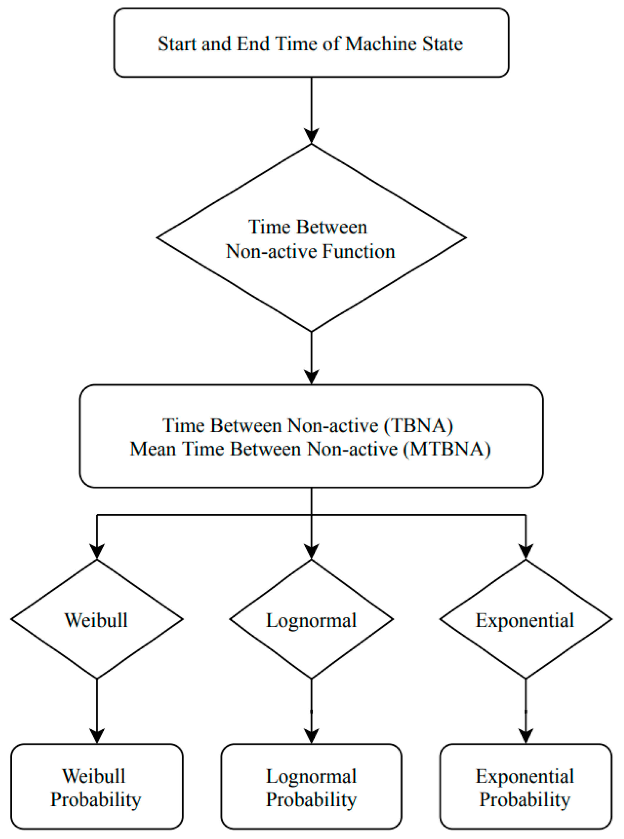Figure 2 illustrates the structure of the reliability analysis.

Based on the TTF [17,18] mathematical formulation, we can define the TBNA state, which is the elapsed time between the non-active states of the machines, and MTBNA as follows.

$$TBNA=startofnon-activetime-startofactivetime$$

(1)

$$MTBNA=\frac{{\displaystyle \sum }TBNA}{number of non-active states}$$

(2)

Once TBNA and MTBNA are calculated, we extract features from raw data using Weibull, lognormal, and exponential distributions. We first obtained the Weibull distribution, which was one of the most widely used lifetime data analyses for reliability engineering [19]. It can flexibly model various types of lifetime distributions [20]. In this paper, we used a 2-parameter Weibull distribution, which had scale and shape parameters. Here, the scale parameter was denoted as $\eta$, and the shape parameter was denoted as $\beta$ [21]. When $\beta$ was less than 1, the distribution showed a decreasing failure rate over time [22]. When $\beta$ was 1, the distribution had a constant failure rate. When the $\beta$ parameter was greater than 1, the failure rate increased over time [21]. We estimated the appropriate scale and shape parameters of the Weibull distribution by using the TBNA with maximum likelihood estimation (MLE) method. More specifically, the MLE formula [23] for determining the parameters of the Weibull distribution is written as follows:

$$\begin{gathered} \beta ={\left[\frac{{{\displaystyle \sum }}_{i=1}^n{t}_i\ln \left(t_i\right)}{{{\displaystyle \sum }}_{i=1}^n{t}_i}-\frac{{{\displaystyle \sum }}_{i=1}^n\ln \left(t_i\right)}{n}\right]}^{-1} \\ \eta ={\left(\frac{1}{n}{\displaystyle \sum }_{i=1}^n{t}_i\right)}^{\frac{1}{\beta }} \end{gathered}$$

(3)

In Equation (3), $t_i$ was TBNA calculated in Equation (1), and $i$ and $n$ are the numbers of non-zero data points. Once the shape parameter $\beta$ and scale parameter $\eta$ of the Weibull distribution was calculated using Equation (3), we could estimate the non-active state rate of the machine using the probability density function of the Weibull as follows:

$$f\left(t\right)=\frac{\beta }{\eta }{\left(\frac{t}{\eta }\right)}^{\beta -1}{e}^{-{\left(t/\eta \right)}^{\beta }}$$

(4)

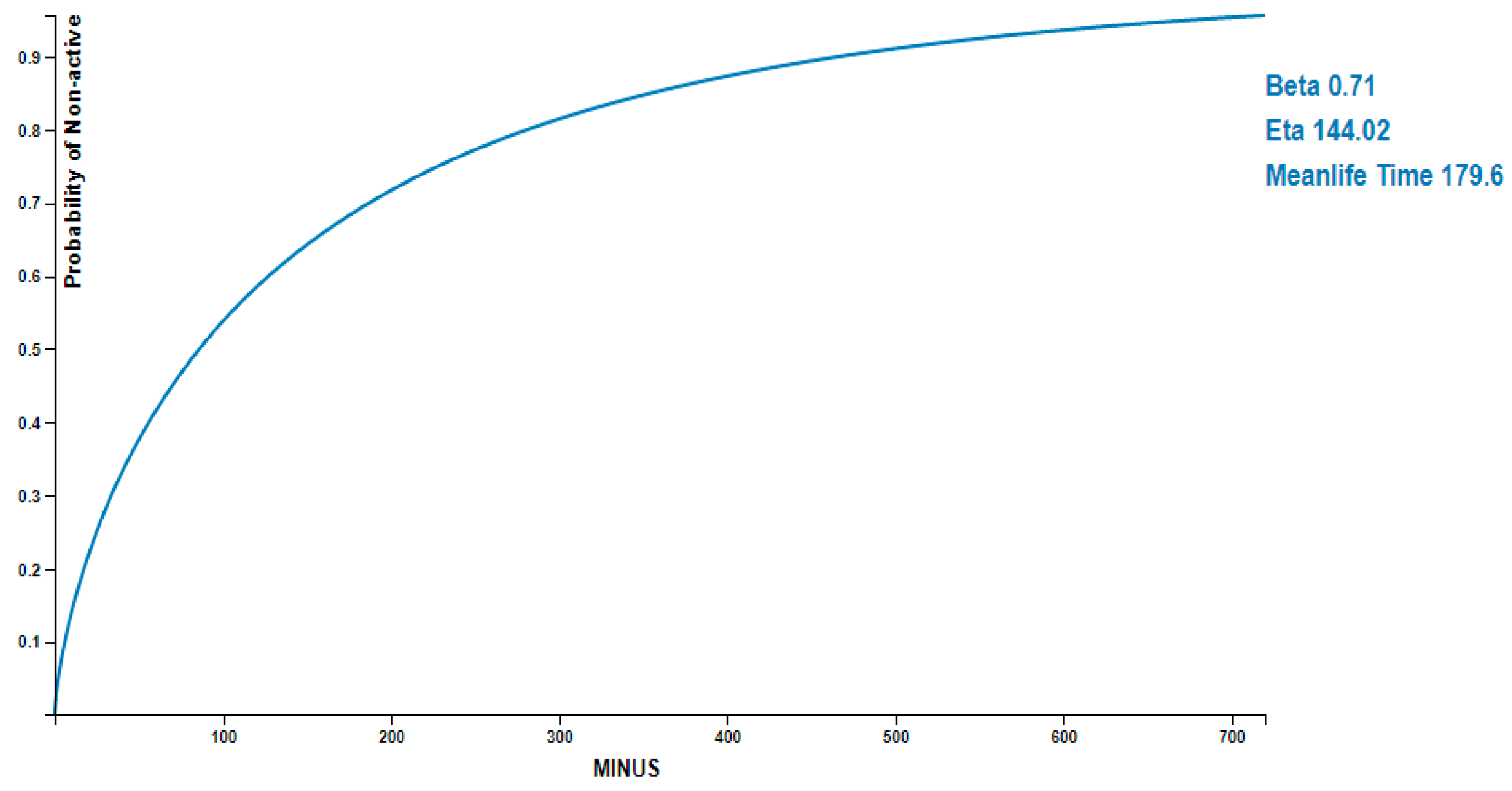
Figure 3 illustrates the fitting curve result of the Weibull distribution with 2 parameters set as $\beta =0.71$, eta $\eta =144.02$, and the mean life of the non-active state was set as 179.6, which means that the non-active state of the machine will occur when the machine was operating for approximately 179 min. In Figure 3, the x-axis indicated the elapsed time (in minutes) from which the machine was active, and the y-axis indicated the probability of the non-active state of the machine. From the figure, we can observe the relationship between active and non-active states of the machine. For example, when the probability of non-activation of a facility was 0.8, it means that about 280 min have passed from the time it was activated.

Further, we obtained the lognormal distribution, which was a constant probability distribution of random variables [24]. This distribution was also widely used to model the lives of units whose failure modes were of the fatigue–stress nature [25]. Additionally, the lognormal distribution complements the Weibull distribution well for modeling the reliability of a machine. The formula of the lognormal distribution is written as follows:

$$f\left(t^{\prime }\right)=\frac{1}{{\sigma }^{\prime }\sqrt{2\pi }}{e}^{-\frac{1}{2}{\left(\frac{t^{\prime }-{\mu }^{\prime }}{{\sigma }^{\prime }}\right)}^2},$$

(5)

In Equation (5), $t^{\prime }$ is $ln\left(t\right)$, where $t$ is TBNA calculated in Equation (1), ${\mu }^{\prime }$ the logarithm of MTBN calculated in Equation (2), and ${\sigma }^{\prime }$ the standard deviation of the natural logarithms of TBNA.

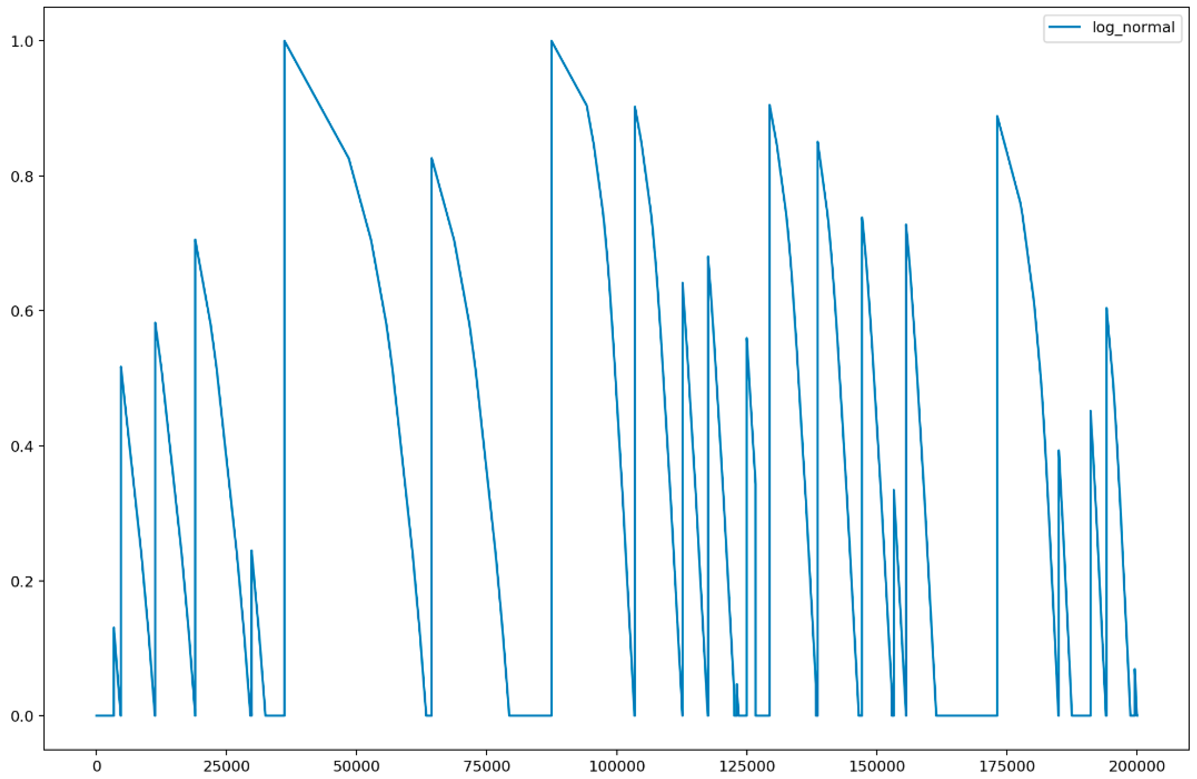
Figure 4 shows the result of lognormal distribution probability. In Figure 4, the x-axis indicated the elapsed time (in minutes) from which the machine was active, and the y-axis indicated the probability of the non-active state of the machine obtained using the lognormal distribution in Equation (5). From the figure, we can observe that a machine enters active and non-active states over time. Here, if the value on the y-axis was 1, the machine was activated, and if the value was close to 0.0, the probability of non-activation increased. In other words, we can see that lognormal distribution is used to describe the probability of a specific event occurring.

Similar to the Weibull and lognormal distributions, the exponential distribution was typically used in reliability engineering and exhibited a simple distribution [26]. The exponential distribution was utilized to model the behavior of units that have a constant failure rate. The primary probability density function for the exponential distribution is expressed as follows.

$$f\left(t\right)=\lambda e^{-\lambda t}=\frac{1}{m}{e}^{-\frac{1}{m}t},t\ge 0,\lambda >0,m>0,$$

(6)

In Equation (6), $\lambda =1/m$ is the constant rate in the non-active state per unit of measurement, $m$ the mean TBNA, and $t$ the TBNA during the machine operation.

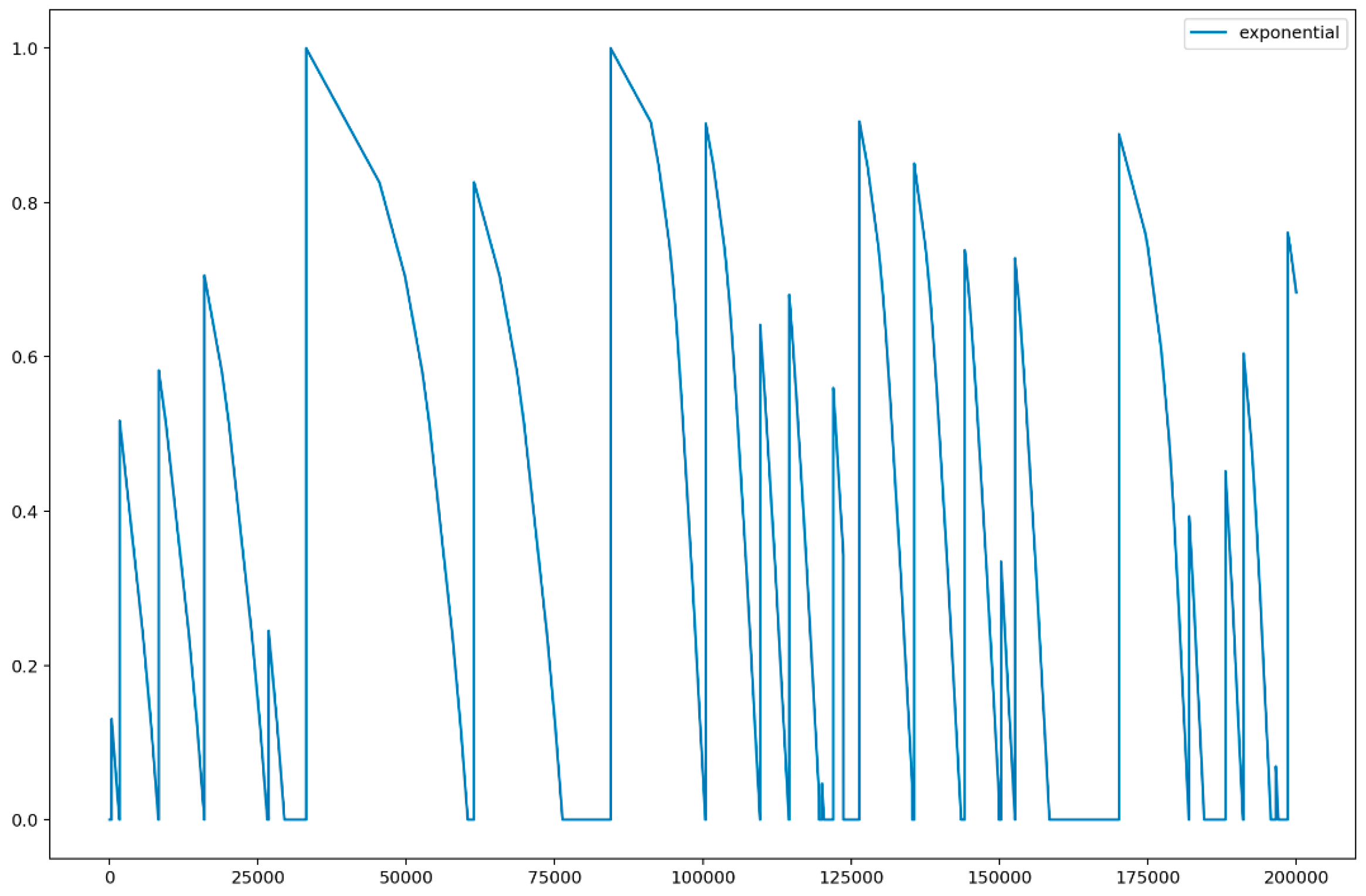
Figure 5 illustrates the result of the exponential distribution. In Figure 5, the x-axis indicated the elapsed time (in minutes) from which the machine was active, and the y-axis indicated the probability of a non-active state of the machine obtained using exponential distribution in Equation (6). Similar to Figure 4, Figure 5 demonstrated that a machine entered active and non-active states over time. Unlike lognormal distributions, the exponential distribution model the time elapsed between events and represented the amount of time until the machine enters into a non-active state.

In feature extraction using reliability analysis, we extracted 4 features, including TBNA, Weibull probability, lognormal probability, and exponential probability. These 4 features will be used later to model the prediction of the non-active state of machines.

Table 2. Reliability Feature Extraction.

Feature	Description	Data Type
Time Between Non-active States	Time elapsed between non-active states	Int
Weibull Distribution	Probability of non-active states occurring during machine operation	Float
Lognormal Distribution		Float
Exponential Distribution		Float

shows the 4 elements extracted from the reliability analysis.

3.2.2. MSTV Features

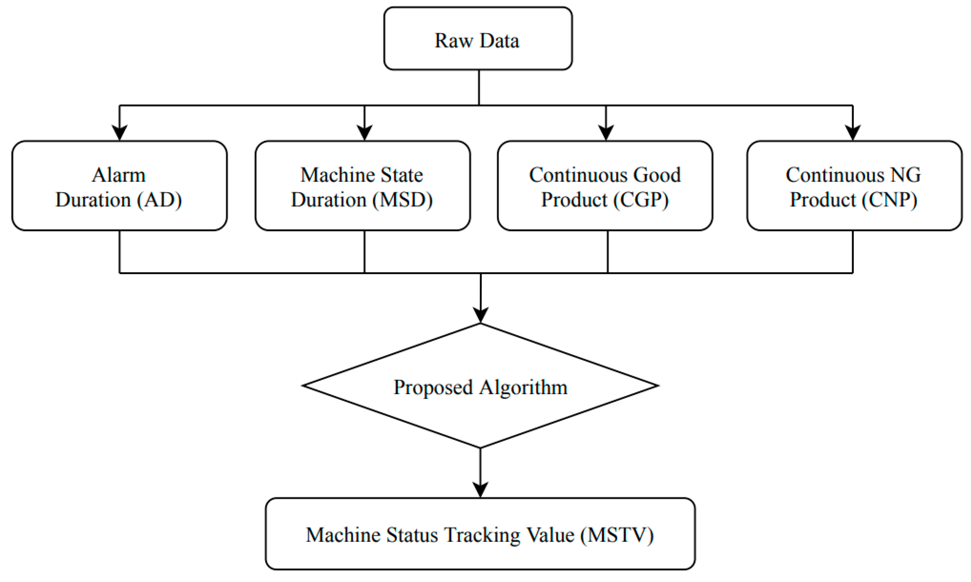
To distinguish the active and non-active patterns of the machine more effectively, we proposed a method to combine various essential factors from the raw dataset related, i.e., the alarm duration (AD), machine state duration (MSD), continuous good product (CGP), and continuous NG product (CNP) to extract new features that can learn the machine’s behavior during operation. We call these features an MSTV. Figure 6 shows the architecture of the proposed feature extraction.

Kang et al. [27] proposed the detection of significant arms using outlier detection algorithms, which indicated the importance of alarm for tracking the behavior of a machine, particularly during the occurrence of an unusual event. Hence, in this experiment, we retrieved the AD during operation as a combined feature for extracting the new useful feature. Meanwhile, the machine duration (MD) provided beneficial information for verifying the behavior of the machine because it indicated the time required by the machine to change from one state to another. Recall from Section 3.1 that a machine can have the following 5 states: Run, wait, stop, offline, and manual, among which run and wait were considered as active states, and stop, offline and manual were considered as non-active states. The CGP means the number of high-quality products produced. The CNP was the quantity of poor-quality products produced.

Based on these 4 features, we define MSTV as follows:

$$MSTV=\Sigma \left(AD\times w1+MSD\times w2+CGP\times w3+CNP\times w4\right)\times \frac{1}{n},$$

(7)

In Equation (7), $w1$, $w2$, $w3,$ and $w4$ are weight values assigned to each factor, respectively. Here, the weight values indicate the importance of the factors that influence the non-active state of the machines. In this case, the importance was determined through discussions with the operators in the factory, and the most important factors were determined as the MSD, followed by the AD. Next was the number of normal products continuously and the number of abnormal products continuously produced by the machine. In consideration of these factors, in this paper, weights were given as 2, 3, 1.5, and 1, respectively.

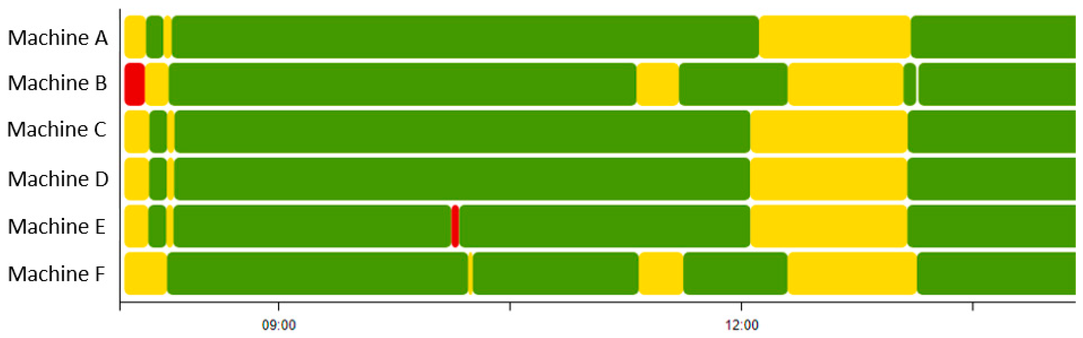
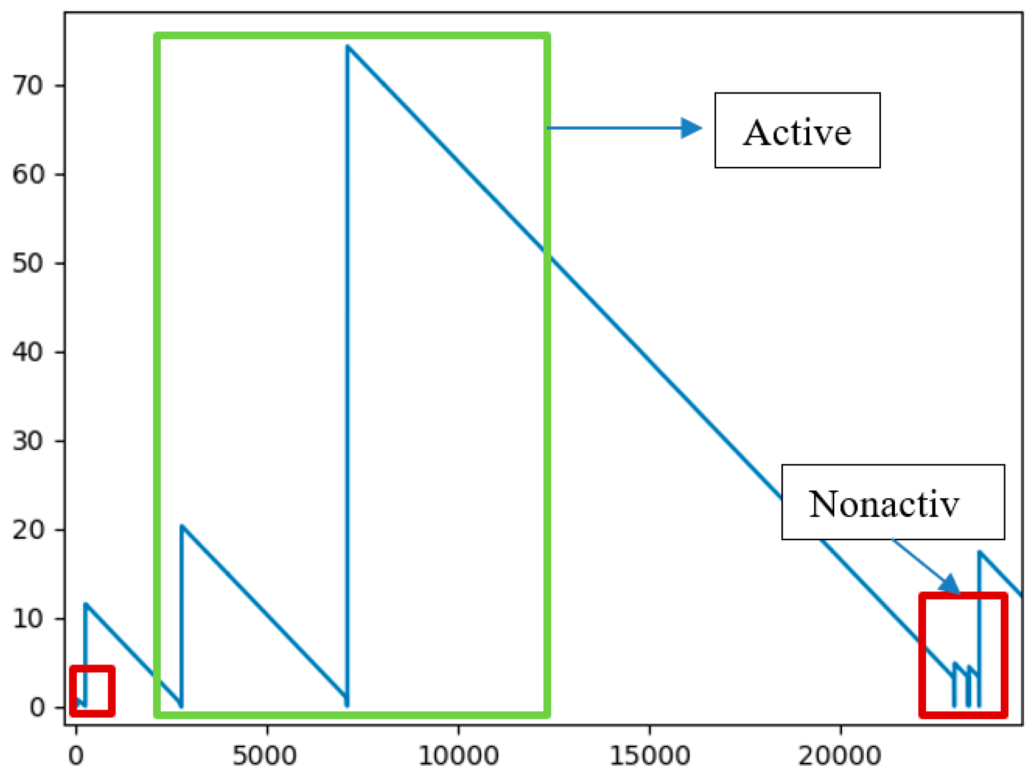
Figure 7 shows the results of MSTV feature extraction. In Figure 7, the x-axis indicated the elapsed time (in minutes) from which the machine was active, and the y-axis indicated the probability of a non-active state of the machine obtained using MSTV in Equation (7). From the figure, we can observe that if the value was close to 0 (indicated in red rectangles), the probability of non-activation increased. On the other hand, we can see that the active state (green rectangle) occurred as the probability curve of MSTV goes higher. As shown in Figure 7, after employing the proposed feature extraction approach to extract the MSTV, the patterns of the active and non-active states of the machine can be distinguished well by combining 4 indispensable elements from the raw dataset to extract new utilitarian features.

3.2.3. Time and Frequency Domain Features

Once MSTV features were obtained using Equation (7), it was applied to the time and frequency domain analyses to extract the other 8 features to enhance the accuracy of our non-active state prediction model. The time-domain analysis employed mathematical functions to analyze physical signals or time-series data with respect to time [28]. Additionally, the time-domain represented the change of a signal with time. Frequency analysis was the statistical method used for measuring the signals with respect to frequency. Frequency analysis typically involved the central tendency, dispersion, and percentiles [29,30]. Figure 8 shows the structure of feature extraction in the time-frequency and domain frequency features.

In the time-domain analysis, several statistical features were used that encompassed a wide range of popular time-domain analyses [6]. These statistical features included the mean value (MV), root mean square value (RMSV), square mean root value (SMRV), kurtosis coefficient (KC), shape factor (SF), and skewness coefficient (SC), which will be utilized to extract the new features from the MSTV. In addition, the root mean square frequency (RMSF) and root variance frequency (RVF), which are obtained from the frequency-domain analysis, will be used to extract two other features from the MSTV data. The details of 8 statistical methods for extracting features from the MSTV are listed in

Table 3. Eight Statistical Features of MSTV.

Features	Equation	Data Type
Time-Domain Analysis
Mean Value	$X_{mv}=\frac{1}{N}{\displaystyle \sum _{i=1}^N}X\left(t_i\right)$	Float
Root-mean-square Value	$X_{rmsv}=\sqrt{\frac{1}{N}{\displaystyle \sum _{i=1}^N}{X}^2\left(t_i\right)}$	Float
Square-mean-root Value	$X_{smrv}={\left[\frac{1}{N}{\displaystyle \sum _{i=1}^N}\sqrt{\left|X\left(t_i\right)\right|}\right]}^2$	Float
Skewness Coefficient	$X_{sc}=\frac{1}{X_{rmsv}{}^3}{\displaystyle \sum _{i=1}^N}{\left(X\left(t_i\right)-X_{mv}\right)}^3$	Float
Kurtosis Coefficient	$X_{kc}=\frac{1}{X_{rmsv}{}^4}{\displaystyle \sum _{i=1}^N}{\left(X\left(t_i\right)-X_{mv}\right)}^4$	Float
Shape Factor	$X_{sf}=\frac{X_{rmsv}}{\frac{1}{N}{{\displaystyle \sum }}_{i=1}^N\left|X\left(t_i\right)\right|}$	Float
Frequency-Domain Analysis
Root Mean Square Frequency	$X_{rmsf}=\sqrt{\frac{{{\displaystyle \sum }}_{i=2}^N{X}^2\left(t_i\right)}{4{\pi }^2{{\displaystyle \sum }}_{i=1}^N{X}^2\left(t_i\right)}}$	Float
Root Variance Frequency	$X_{rvf}=\sqrt{\frac{{{\displaystyle \sum }}_{i=2}^N{X}^2\left(t_i\right)}{4{\pi }^2{{\displaystyle \sum }}_{i=1}^N{X}^2\left(t_i\right)}-{\left(\frac{{{\displaystyle \sum }}_{i=1}^N{X}^2\left(t_i\right)}{2\pi {{\displaystyle \sum }}_{i=1}^N{X}^2\left(t_i\right)}\right)}^2}$	Float

.

3.3. Data Normalization

Data normalization was one of the essential preprocessing steps for many machine learning algorithms. Raw data and extracted features often have different scales. In other words, the variation between features can be inconsistent, which may result in many problems during data training, including lowering accuracy and increasing the training time. The normalization process for data contributed positively to preparing data that were suitable for training [31]. Moreover, data normalization can scale the data in the same range of values for each input feature to minimize bias in the input data. Furthermore, data normalization can also accelerate the training time by starting the training operation for each feature within the same scale. Various types of data normalization methods can be employed to reduce the bias of the training data, such as the Min-Max Normalization, Z-Score Normalization, Sigmoid Normalization, and others.

In our case, after feature extraction using statistical analysis described in Section 3.2, 17 input features were obtained, including raw data from the sensor device. The variations between the input features were large and diverse, which may cause problems in the training phase. Thus, we needed to normalize the data. We used Min-Max Normalization that rescaled the features from one range of values to a new range of values. Typically, the features were rescaled within a range of 0 to 1 or from −1 to 1.

Table 4. Sample training dataset.

No	MSD	CGP	CNP	TBNA	Weibull Probability	Exponential Probability	Lognormal Probability	MSTV	MV	RMSV	SMRV	SC	KC	SF	RMSF	RVF
1	0.396938	0.603901	0.073171	0.396938	0.711354	0.603363	0.999969	0.437343	0.437343	1.91286 × 10−1	0.437343	8.321303 × 10−15	1.686249 × 10−19	8.364994 × 10−2	0.046755	9.948226 × 10−3
2	0.000000	0.000000	0.000000	0.000000	0.000000	0.000000	0.000000	0.000000	0.000000	0.000000	0.000000	0.000000	0.000000	0.000000	0.000000	0.000000
3	0.234286	0.342357	0.024390	0.234322	0.451382	0.332008	0.999919	0.256797	0.256797	6.594449 × 10−2	0.256797	4.110406 × 10−14	1.418555 × 10−18	1.693450 × 10−2	0.034228	2.510931 × 10−3
4	0.000110	0.000000	0.000000	0.000000	0.000000	0.000000	0.000000	0.000080	0.000080	6.361941 × 10−9	0.000080	1.371742 × 10−3	1.524158 × 10−4	5.074397 × 10−13	0.000014	4.571769 × 10−11
5	0.460787	0.421576	0.032520	0.460787	0.881584	0.823336	0.999987	0.482576	0.482576	2.328801 × 10−1	0.482576	6.193819 × 10−15	1.137482 × 10−19	1.123824 × 10−1	0.215370	5.579461 × 10−2
6	0.026436	0.000000	0.000000	0.000000	0.000000	0.000000	0.000000	0.012762	0.012762	1.628657 × 10−4	0.012762	3.348980 × 10−10	2.325680 × 10−13	2.078473 × 10−6	0.000573	1.038138 × 10−7
7	0.001248	0.251990	0.056911	0.001248	0.005749	0.003356	0.999202	0.023893	0.023893	5.708795 × 10−4	0.023893	5.103174 × 10−11	1.892869 × 10−14	1.364007 × 10−5	0.003060	1.943214 × 10−6
8	0.078352	0.122611	0.000000	0.078389	0.155148	0.097674	0.999810	0.086568	0.086568	7.494039 × 10−3	0.086568	1.072959 × 10−12	1.098443 × 10−16	6.487448 × 10−4	0.000437	3.645383 × 10−6
9	0.208805	0.000000	0.000000	0.000000	0.000000	0.000000	0.000000	0.151202	0.151202	2.286197 × 10−2	0.151202	2.013662 × 10−13	1.180272 × 10−17	3.456769 × 10−3	0.093885	2.387736 × 10−3
10	0.208805	0.289809	0.024390	0.176494	0.395984	0.282752	0.999915	0.196320	0.196320	3.854167 × 10−2	0.196320	9.199435 × 10−14	4.152869 × 10−18	7.566513 × 10−3	0.043935	1.883721 × 10−3
11	0.176494	0.648487	0.024390	0.045932	0.180633	0.115217	0.999711	0.091531	0.091531	8.377937 × 10−3	0.091531	9.077188 × 10−13	8.788911 × 10−17	7.668416 × 10−4	0.010724	9.994741 × 10−5
12	0.034880	0.000000	0.000000	0.000000	0.000000	0.000000	0.000000	0.000000	0.000000	0.000000	0.000000	0.000000	0.000000	0.000000	0.000000	0.000000
13	0.009289	0.000000	0.000000	0.000000	0.000000	0.000000	0.000000	0.006727	0.006727	4.524683 × 10−5	0.006727	2.287045 × 10−9	3.013234 × 10−12	3.043563 × 10−7	0.002244	1.127246 × 10−7
14	0.017367	0.000000	0.000000	0.017403	0.938259	0.905281	0.999816	0.016768	0.016768	2.811557 × 10−4	0.016768	1.476511 × 10−10	7.803968 × 10−14	4.714334 × 10−6	0.004492	1.404966 × 10−6
15	0.000000	0.000000	0.000000	0.000000	0.000000	0.000000	0.000000	0.000000	0.000000	0.000000	0.000000	0.000000	0.000000	0.000000	0.000000	0.000000

shows the application Min-Max Normalization on a sample training dataset, which is calculated using the following formula:

$$x^{\prime }=\left(x_{max}-x_{min}\right)\times \frac{\left(x_i-x_{min}\right)}{x_{max}-x_{min}}+x_{min}$$

(8)

In Equation (8), i is ith element of the dataset.

3.4. Model Training

Once statistical features were extracted and data normalized, learning models for predicting non-active states of the machines were constructed by combining the raw data from the sensor device and extracted features. Considering that we deal with a dataset that contains active and non-active states, we can formulate the predicting non-active states of machines as a classification problem. Thus, we constructed predictive models using the following state-of-the-art machine learning methods suitable for classification: Decision tree, kNN, random forest, and linear SVM.

A decision tree is one of the most popular methods used for classification. The decision tree predicts the class of a target feature by producing simple decision rules inferred from the data [32]. In the context of the proposed method, these decision rules enabled us to understand and interpret non-active states of machines easily. kNN classification was one of the most fundamental and simple classification methods. It classifies the class of a target feature by using the distance between a test sample and the specified training samples [33]. kNN is suitable for datasets with numeric values. Thus, it can be easily adapted for our dataset as it contains numeric values obtained through statistical analysis. Breiman [34] introduced the random forest method, which was a combination of tree predictors. In other words, a random forest algorithm creates a decision tree on data samples, gets the prediction from each of them, and finally selects the best solution. Despite its complexity, the random forest algorithm achieves high accuracy because it creates multiple trees and enables us to choose a tree with the highest accuracy. Considering that predicting the non-active status of machines with high accuracy can bring benefits to the efficient production of manufacturing machines, we can efficiently utilize the random forest algorithm to solve our problem. SVM was another classification method that was widely used for the analysis of a large amount of data. One of the main advantages of SVM was that it was effective in high dimensional spaces. In the case of our dataset, we obtained 17 input features, including raw data from the sensor device. Considering that the proposed dataset was relatively high dimensional, we can benefit from using SVM for classifying the non-active state of the machines.

Table 5. The pros and cons of classification methods.

Method	Pros	Cons
Decision Tree	●    Simple to understand and to interpret	●    Easy overfitting.
	●    Requires little data preparation	●    The greedy algorithm
	●    Handle numerical and categorical data	●    Can be unstable
KNN	●    Simple to understand and to interpret	●    A bit expensive algorithm
	●    Useful for non-linear data	●    High memory storage required.
	●    A versatile algorithm	●    Very sensitive
Random Forest	●    Overcomes the problem of overfitting	●    Complexity
	●    Very flexible	●    More computational resources are required
	●    Less variance than single decision tree
Linear SVM	●    Effective in high dimensional spaces.	●    Easy to overfitting
	●    Memory efficient	●    Do not directly provide probability estimates
	●    Versatile

demonstrate the advantages and disadvantage of classification algorithm used in this study.

4. Performance Evaluation

4.1. Experimental Setup

The methods and techniques to select the appropriate operating pattern subject to the optimal value of power per product quantity are described herein. In addition, to obtain the experimental results, we used a computer with a CPU Intel^® Core™ i7-6700 3.40 GHz, 32 GB of RAM, NVIDIA GeForce 9800 GT graphics card, Windows 10 operating system, and an integrated development environment Jupyter notebook for Python and IntelliJ for Java. Moreover, the Maria database was used to store a large amount of data.

4.2. Hyperparameter of Competing Methods

Recall from Section 3.4 that we constructed predictive models using a decision tree, kNN, random forest, and linear SVM.

Table 6. The hyperparameters of competing methods.

Algorithm	Parameters
Decision Tree	class_weight	None
	criterion	gini
	max_depth	None
	max_features	None
	max_leaf_nodes	None
	min_impurity_decrease	0.0
	min_impurity_split	None
	min_samples_leaf	1
	min_samples_split	2
	min_weight_fraction_leaf	0.0
	presort	False
	random_state	None
	splitter	best
KNN	algorithm	auto
	leaf_size	30
	metric	minkowski
	metric_params	None
	n_jobs	None
	n_neighbors	5
	p	2
	weights	uniform
Random Forests	class_weight	None
	criterion	gini
	max_depth	None
	max_features	None
	max_leaf_nodes	None
	min_impurity_decrease	0.0
	min_impurity_split	None
	min_samples_leaf	1
	min_samples_split	2
	min_weight_fraction_leaf	0.0
	presort	False
	random_state	None
	splitter	best
Linear SVM	C	10
	class_weight	None
	dual	True
	fit_intercept	True
	intercept_scaling	1
	loss	squared_hinge
	max_iter	1000
	multi_class	ovr
	penalty	l2
	random_state	None
	tol	0.0001
	verbose	0

demonstrates a detailed description of each hyperparameter of competing methods. Various combinations of the parameters were applied in the experiments, and the most optimum set was selected. First, the prediction of the non-active state of machines with a decision tree was performed using the Gini impurity. Further, the kNN model was constructed using the Minkowski distance to compute the distance between an observation data point and its nearest neighbors with k = 5. Here, we tested various combinations of k and selected as k = 5 because it produced the highest accuracy. Moreover, utilizing the advantage of the bagging method, the random forest was developed using the Gini impurity. Finally, the radial basis function, a kernel SVM, was employed to map the data into a high-dimensional space. Here, the C parameter, which controls the penalty of the data points outside the margin, was set to 10. Similar to the k parameter of kNN, we tested various combinations of C parameter and selected as C = 10 as it produced the highest accuracy.

4.3. Evaluation Metrics

The four machine learning methods were validated based on the root mean square error (RMSE), precision and recall scores, and F1 scores.

We first describe the RMSE. The RMSE computes the variance between values predicted by a hypothetical model and the real values. In other words, it measures the standard-of-fit between the actual data and the predicted model. It is expressed as follows:

$$RMSE=\sqrt{\frac{{{\displaystyle \sum }}_{i=1}^n{\left(\widehat{y_i}-y_i\right)}^2}{n}},$$

(9)

In Equation (9), $\widehat{y_i}$ is the predicted variable, $y_i$ the actual variable, and $n$ the number of observations. The RMSE is always non-negative. In general, a lower RMSE is better.

Precision, recall, and F1 score are measurements to check the accuracy of training models. Specifically, precision is a measure of result relevancy, whereas recall represents the degree to which many genuinely relevant results are returned. Meanwhile, the F1 score is calculated using the values obtained from precision and recall. Precision, recall, and F1 score are expressed as follows:

$$\begin{gathered} Precision=\frac{{{\displaystyle \sum }}_{i=1}^{n}TP/\left(TP+FP\right)}{n} \\ Recall=\frac{{{\displaystyle \sum }}_{i=1}^{n}TP/\left(TP+FN\right)}{n} \\ {F}_1 score=\frac{TP}{TP+\frac{1}{2}\left(FP+FN\right)} \end{gathered}$$

(10)

In Equation (10), TP, FP, and FN indicate true positive, false positive, and false negative, respectively; $n$ represents the total amount of observation data.

4.4. Experimental Results

Table 7. Model Comparison Result.

Model	Precision	Recall	F1 Score	Observations	RMSE
Decision tree	92%	75%	83%	86,400	0.3478
KNN	93%	95%	94%	86,400	0.2085
Random forest	96%	85%	90%	86,400	0.1813
Linear SVM	98%	99%	98%	86,400	0.0677

presents the experimental results. Here, for the training dataset, we used 86,400 samples, where 73,019 active states and 13,381 non-active states were detected.

From the table, we can observe that linear SVM achieved 98% accuracy in terms of F1 score in the classification of non-active states of machines, followed by kNN, random forest, and decision tree, which were only 94%, 90%, and 83%, respectively. We can also observe from the table that linear SVM also achieved the lowest error rate (i.e., 0.0677) compared with other methods. Linear SVM used two hyperplanes that separated the observations linearly, thus that there were no observations between them. Linear SVM performed better than other methods in our experiments as the dataset has been constructed using features that are suitable for creating linearly-separable observations. On the other hand, the random forest also performed well, which resulted in accuracy close to SVM in terms of precision. Random forest is a well-known knowledge-based ensemble method that overcomes the overfitting problem as well as errors due to bias in the decision tree and, therefore, yields high accuracy. As kNN is not a knowledge-based ensemble technique like the random forest, it achieves marginally less accurate results but still outperforms the decision tree in terms of precision, recall, and F1 score.

Figure 8 demonstrates the visualized result of SVM. In Figure 9a,b, we can see machine states for a single day. Here, the blue line indicates the actual machine state (in every second), and the red line indicates predicted machine states (in every second) using linear SVM. From the figures, it is clear that the prediction by linear SVM follows the actual machine state well. On the other hand, the result also suggests that there were some errors (e.g., approximately at 02:00, 04:00, or 05:30) in the prediction process. However, a closer look for these errors indicated that wrongly predicted observations were short-term (a matter of seconds) and, therefore, were insignificant to the overall prediction of non-active state predictions.

5. Conclusions

In this paper, a combination of various statistical methods and machine learning have been proposed to predict the active and non-active states of the machine. In this approach, reliability analysis, the proposed feature extraction method MSTV, as well as time- and frequency-domain analyses, were used to extract features from a raw dataset. Hence, 17 useful features were obtained in the extraction phase, including Weibull, lognormal, and exponential probability distributions, and the proposed feature extraction the MV, RMSV, SMRV, KC, SF, SC, which will be utilized to extract the new features from the MSTV. In addition, RMSF and RVF. Furthermore, after normalization, we used to train four types of machine learning, i.e., the decision tree, kNN, random forest, and a linear SVM model to detect the active and non-active states of the machine. According to the experimental results, the linear SVM model’s predicted result indicated a 98% accuracy rate compared with the actual value; this demonstrated that the model was highly accurate and, therefore, can be utilized to reduce machine faults and increase productivity.

Even though the performance of the non-active state detection model was satisfactory with high accuracy, the statistical method to extract the train features was conservative, and the detection model could not solve all the issues encountered in manufacturing. Therefore, in the future, we plan to utilize more statistical methods such as the Hilbert–Huang Transform or the fast Fourier transform along with the proposed approach to extract more valuable features and develop a promising non-active state prediction model. Finally, we will attempt to create a user-friendly interface for displaying the results in a web application platform.

References

1. Perry, R.H.; Green, D.W. Perry’s Chemical Engineers’ Handbook, 7th ed.; McGraw-Hill: New-York, NY, USA, 1997. [Google Scholar]
2. Ahmad, S.; Badwelan, A.; Ghaleb, A.M.; Qamhan, A.; Sharaf, M.; Alatefi, M.; Moohialdin, A. Analyzing Critical Failures in a Production Process: Is Industrial IoT the Solution? Wirel. Commun. Mob. Comput. 2018, 2018, 6951318. [Google Scholar] [CrossRef]
3. Boutros, T.; Liang, M. Detection and diagnosis of bearing and cutting tool faults using hidden Markov models. Mech. Syst. Signal. Process. 2011, 25, 2102–2124. [Google Scholar] [CrossRef]
4. Çınar, Z.M.; Abdussalam Nuhu, A.; Zeeshan, Q.; Korhan, O.; Asmael, M.; Safaei, B. Machine Learning in Predictive Maintenance towards Sustainable Smart Manufacturing in Industry 4.0. Sustainability 2020, 12, 8211. [Google Scholar] [CrossRef]
5. Angelopoulos, A.; Michailidis, E.T.; Nomikos, N.; Trakadas, P.; Hatziefremidis, A.; Voliotis, S.; Zahariadis, T. Tackling Faults in the Industry 4.0 Era—A Survey of Machine-Learning Solutions and Key Aspects. Sensors 2020, 20, 109. [Google Scholar] [CrossRef] [PubMed] [Green Version]
6. Wu, J.; Wu, C.; Cao, S.H.; Or, S.W.; Deng, C.; Shao, X. Degradation Data-Driven Time-To-Failure Prognostics Approach for Rolling Element Bearings in Electrical Machines. IEEE Trans. Ind. Electron. 2019, 66, 529–539. [Google Scholar] [CrossRef]
7. Zhou, Z.; Wen, C.; Yang, C. Fault Detection Using Random Projections and k-Nearest Neighbor Rule for Semiconductor Manufacturing Processes. IEEE Trans. Semicond. Manuf. 2015, 28, 70–79. [Google Scholar] [CrossRef]
8. Mazhar, M.I.; Kara, S.; Kaebernick, H. Remaining life estimation of used components in consumer products: Life cycle data analysis by Weibull and artificial neural networks. J. Oper. Manag. 2007, 25, 1184–1193. [Google Scholar] [CrossRef]
9. Shenfield, A.; Howarth, M. A Novel Deep Learning Model for the Detection and Identification of Rolling Element-Bearing Faults. Sensors 2020, 20, 5112. [Google Scholar] [CrossRef]
10. Luo, B.; Wang, H.; Liu, H.; Li, B.; Peng, F. Early Fault Detection of Machine Tools Based on Deep Learning and Dynamic Identification. IEEE Trans. Ind. Electron. 2019, 66, 509–518. [Google Scholar] [CrossRef]
11. He, Q.P.; Wang, J. Principal component based k-nearest-neighbor rule for semiconductor process fault detection. In Proceedings of the American Control Conference (ACC), Seattle, WA, USA, 11–13 June 2008; pp. 1606–1611. [Google Scholar]
12. Rumelhart, D.E.; McClelland, J.L. Learning Internal Representations by Error Propagation. In Parallel Distributed Processing: Explorations in the Microstructure of Cognition: Foundations; MIT Press: Cambridge, MA, USA, 1987; pp. 318–362. [Google Scholar]
13. Bengio, Y.; Lecun, Y. Convolutional Networks for Images, Speech, and Time-Series. In The Handbook of Brain Theory and Neural Networks; MIT Press: Cambridge, MA, USA, 1998; pp. 255–258. [Google Scholar]
14. Iqbal, R.; Maniak, T.; Doctor, F.; Karyotis, C. Fault Detection and Isolation in Industrial Processes Using Deep Learning Approaches. IEEE Trans. Industr. Inform. 2019, 15, 3077–3084. [Google Scholar] [CrossRef]
15. Dey, A.K.; Kundu, D. Discriminating Among the Log-Normal, Weibull, and Generalized Exponential Distributions. IEEE Trans. Reliab. 2009, 58, 416–424. [Google Scholar] [CrossRef] [Green Version]
16. Armor, D.J. Theta Reliability and Factor Scaling. Sociol. Methodol. 1974, 5, 17–50. [Google Scholar] [CrossRef]
17. Dai, Y.; Zhou, Y.; Jia, Y. Distribution of time between failures of machining center based on type I censored data. Reliab. Eng. Syst. Saf. 2003, 79, 377–379. [Google Scholar] [CrossRef]
18. Kimura, M.; Yamada, S.; Osaki, S. Statistical Software Reliability Prediction and Its Applicability Based on Mean Time between Failures. Math. Comput. Model. 1995, 22, 149–155. [Google Scholar] [CrossRef]
19. Liu, C. A Comparison Between the Weibull and Lognormal Models Used to Analyse Reliability Data. Ph.D. Thesis, University of Nottingham, Nottingham, UK, 1997. [Google Scholar]
20. Kundu, D.; Gupta, R.D.; Manglick, A. Discriminating between the log-normal and generalized exponential distributions. J. Stat. Plan. Inference 2005, 127, 213–227. [Google Scholar] [CrossRef]
21. Tiryakioğlu, M.; Hudak, D. Guidelines for Two-Parameter Weibull Analysis for Flaw-Containing Materials. Metall. Mater. Trans. B 2011, 42, 1130–1135. [Google Scholar] [CrossRef]
22. Smith, R.L. Maximum Likelihood Estimation in a Class of Non-regular Case. Biometrika 1985, 72, 67–90. [Google Scholar] [CrossRef]
23. Kang, D.; Ko, K.; Huh, J. Comparative Study of Different Methods for Estimating Weibull Parameters: A Case Study on Jeju Island, South Korea. Energies 2018, 11, 356. [Google Scholar] [CrossRef] [Green Version]
24. Aitchison, J.; Brown, J.A.C. The Lognormal Distribution with Special Reference to Its Uses in Econometrics; Cambridge University Press: New York, NY, USA, 1957. [Google Scholar]
25. Characteristics of the Lognormal Distribution. Available online: https://www.weibull.com/hotwire/issue47/relbasics47.htm (accessed on 16 May 2019).
26. Courant, R.; Robbins, H.; Stewart, I. What is Mathematics? An Elementary Approach to Ideas and Methods, 2nd ed.; Oxford University Press: Oxford, UK, 1996. [Google Scholar]
27. Kang, B.H.; Kim, Y.S.; Chen, Z.; Kim, T. Detecting Significant Alarms using Outlier Detection Algorithms. Adv. Sci. Technol. Lett. 2013, 29, 521–528. [Google Scholar]
28. Lee, Y.W.; Cheatham, T.P.; Wiesner, J.B. Application of Correlation Analysis to the Detection of Periodic Signals in Noise. Proc. IRE 1950, 38, 1165–1171. [Google Scholar] [CrossRef]
29. Boashas, B. Note on the use of the Wigner distribution for time-frequency signal analysis. IEEE Trans. Acoust. Speech Signal. Process. 1988, 36, 1518–1521. [Google Scholar] [CrossRef] [Green Version]
30. What is Frequency Analysis? History and Definition of Frequency Analysis. Available online: https://www.researchoptimus.com/article/frequency-analysis.php (accessed on 17 May 2019).
31. Jayalakshmi, T.; Santhakumaran, A. Statistical Normalization and Back Propagation for Classification. IJCTE 2011, 3, 89–93. [Google Scholar] [CrossRef]
32. Decision Trees. Available online: https://scikit-learn.org/stable/modules/tree.html (accessed on 12 October 2020).
33. Bailey, T.; Jain, A. A note on distance-weighted k-nearest neighbor rules. IEEE Trans. Syst. Man Cybern. 1978, 8, 311–313. [Google Scholar]
34. Breiman, L. Random Forests. Mach. Learn. 2001, 45, 5–32. [Google Scholar] [CrossRef] [Green Version]
Figure 1. Examples of machine operating processes.
Applsci 10 07413 g001
Figure 2. Structure of feature extraction in reliability analysis.
Applsci 10 07413 g002
Figure 3. Result of the fitting curve of Weibull distribution.
Applsci 10 07413 g003
Figure 4. Result of lognormal distribution.
Applsci 10 07413 g004
Figure 5. Result of exponential distribution results.
Applsci 10 07413 g005
Figure 6. Architecture of proposed feature extraction.
Applsci 10 07413 g006
Figure 7. Results of machine status tracking value (MSTV) feature extraction.
Applsci 10 07413 g007
Figure 8. Structure of feature extraction in Time-domain and Frequency-domain features.
Applsci 10 07413 g008
Figure 9. Comparison of the actual and predicted results of the support vector machine (SVM). (a) Actual machine states (in every second). (b) Predicted machine states (in every second) using linear SVM.
Applsci 10 07413 g009