A Comparative Study of MCDM Methods Integrated with Rapid Visual Seismic Vulnerability Assessment of Existing RC Structures

Abstract

Recently, the demand for residence and usage of urban infrastructure has been increased, thereby resulting in the elevation of risk levels of human lives over natural calamities. The occupancy demand has rapidly increased the construction rate, whereas the inadequate design of structures prone to more vulnerability. Buildings constructed before the development of seismic codes have an additional susceptibility to earthquake vibrations. The structural collapse causes an economic loss as well as setbacks for human lives. An application of different theoretical methods to analyze the structural behavior is expensive and time-consuming. Therefore, introducing a rapid vulnerability assessment method to check structural performances is necessary for future developments. The process, as mentioned earlier, is known as Rapid Visual Screening (RVS). This technique has been generated to identify, inventory, and screen structures that are potentially hazardous. Sometimes, poor construction quality does not provide some of the required parameters; in this case, the RVS process turns into a tedious scenario. Hence, to tackle such a situation, multiple-criteria decision-making (MCDM) methods for the seismic vulnerability assessment opens a new gateway. The different parameters required by RVS can be taken in MCDM. MCDM evaluates multiple conflicting criteria in decision making in several fields. This paper has aimed to bridge the gap between RVS and MCDM. Furthermore, to define the correlation between these techniques, implementation of the methodologies from Indian, Turkish, and Federal Emergency Management Agency (FEMA) codes has been done. The effects of seismic vulnerability of structures have been observed and compared.

1. Introduction

Seismic vulnerability assessment of existing structures has always been a significant issue in structural engineering, making it a globally constituted research problem. In today’s rapid urbanization, most of the building stock comprises old constructions or buildings with high importance factors. These structures fail to comply with today’s advanced seismic resistance codes as they were constructed with obsolete seismic design philosophies. Moreover, the ability to assess the seismic vulnerability in real-time presence for a vast number of buildings in the target zone gives rise to the demand for a rapid and reliable screening method. A single seismically vulnerable building can be assessed by a detailed structural assessment such as a non-linear finite element analysis. For a large building stock, an approximate estimate that is efficient in prioritizing the structures for retrofitting shall be sufficient. The primary lateral load resistance system contributes as a significant factor in the structure’s seismic response during earthquake events, as the level of vulnerability differs according to various types of structures. The seismic vulnerability can be defined as the insufficient resistance of the structure to withstand an impact from seismically induced vibrations [1]. First developed in 1988 by the United States as a standard guideline methodology for rapid vulnerability assessment, several national seismic codes were further developed by various other countries worldwide, each of them being specific to local factors of construction methods and design philosophies [2,3]. The codes were further subjected to revisions for the incorporation of the latest advancements in seismic research [4]. The seismic vulnerability assessment can be performed in 3 stages—the initial stage consist of a fundamental walk-down survey followed by the second stage including of a more in-detail structural analysis of the buildings that have failed to achieve the cut-off score in the first stage, and further in the tertiary stage a detailed study on damage inspections, different behavior patterns with a structural analysis [5]. Nevertheless, with a vast number of buildings, due to limited human resources and available funds, a comprehensive investigation of individual buildings is not feasible which highlights the importance of using a simple walk-down survey. Rapid visual screening (RVS) help to classify buildings with varying grades of damage based on seismic vulnerability assessments. This method works with optimum seismic parameters: the age of the building, soil classification, seismic zone, quality the of material, the number of stories, and so forth. RVS is one of the superior methods, though it becomes laborious to run it in the case of missing parameters. This method involves several structural parameters to perform an analysis. In RVS, visualization of parameters is needed during structural assessments, and sometimes it might be problematic due to unhealthy or old constructions. The walk-down survey, however, is prone to the evaluator’s subjectivity, and therefore it is necessary to develop an Multi-criteria based RVS process and tool for screening and prioritizing buildings for further investigations. In addition, the proposed method must take into account the weight and importance of the parameters and cover the uncertainty. Consequently, a supporting decision mechanism is significant to focus on what is essential, logical, compatible, and easy to work. In that scenario, implementing a method known as ‘Multi-Criteria Decision Making’ would help address problems with selected parameters by involving multiple criteria [6]. From past times it can be seen that the concept of decision making is essential for resolving daily life problems, which includes different attributes and activities. Every single activity or attribute cannot resolve a scientific or mathematical approach to make a decision [7]. Multiple decisions have been taken for the majority of tasks or activities from various fields like management, engineering, politics, environment, and business, and so forth according to requirements and experience. There are many solutions available to make a perfect decision, but there would not be a single rule which can make the decision to be perfect. Hence, it needs enormous knowledge, experience, time, money, power, and many other things to make an optimal decision. Multi-Criteria Decision Making (MCDM) helps to make the best decision among several choices available according to decision-makers in every problem [8].

Ebrahimi extensively used hybrid fuzzy methods such as fuzzy TOPSIS and Multiple Objective Decision Making (MODM) [9] for adequate application in regard to the emergency services in Tehran, by conducting a profound analysis based on population density, number of accidents, traffic zone, number of people per emergency, major fault lines, and regional construction to delineate the importance of the places.

Peng [10] assessed the vulnerability of 31 Chinese regions using 6 different MCDM methods that is, TOPSIS, VIKOR, ELECTRE III, PROMETHEE II, grey relational analysis and Weighted Sum Method (WSM) based on 11 criterion such as population, city built-up area, residential families, industries, and so forth. Out of the 6 methods, TOPSIS was the most selected method, because it was the most efficient and trustworthy one. Furthermore, Bana e Costa et al. [11] used MACBETH as the MCDM method for categorizing bridges and tunnels. They prepared an additive aggregation model to calculate final priority scores, and the more the priority values, the higher the importance of the structure. Analytic Hierarchy Process (AHP) and GIS have been used by Rezai and Panahi [12] for creating vulnerability maps of the areas. Caterino and Cosenza [13] proposed an MCDM framework for selecting the seismic retrofit intervention for existing reinforced concrete-frame buildings accounting for expected losses and tax incentives. The developed GIS-AHP model was unable to find a seismic vulnerability for 2 buildings because of insufficient data. Mardani et al. [14] studied 393 articles and 120 journals published from 2000 to 2014 on applications and methods of various MCDM techniques. Their work concluded that the AHP and hybrid MCDM are the most useful methods among individual and integrated approaches, respectively.

As RVS is a discrete problem, and Multiple Attribute Decision-making (MADM) deals with discrete problems as well, few of the MADM methods were selected. Among the MADM approaches, WSM was selected due to its ease of computing and being a basic method that is suitable for single dimensional problems. WPM was selected for multi-dimensional problems, even though RVS is not multi-dimensional. AHP was selected as it is fundamentally easier compared to ELECTRE and PROMOTHEE. ELECTRE is also quite useful, but due to its complexity, TOPSIS was selected instead, which also gives better results as compared to ELECTRE. From the literature review, AHP and TOPSIS give the best results for seismic vulnerability. The more complete the nature of data, the more accurate the results shall. However, an investigation by Caterino et al. [15] for selecting proper strategy on seismic structural retrofitting figured out TOPSIS and VIKOR are appropriate methods for solving the retrofit selection problem.

In this paper, the goal is to show the reliability of MCDM used for a seismic vulnerability assessment, specifically to classify the damage index of reinforced concrete (RC) buildings using the RVS method, which also prioritizes the buildings for further evaluations. For this purpose, three common RVS methods have been selected, and the importance of the building’s performance modifiers by each of them has been investigated. Based on their preference, they received ranking and corresponding weight of importance. Later, according to their value of importance applied to different MCDM methods and the data of 28 RC buildings in Bingöl, Turkey, has been employed to estimate the damage grades by each applied MCDM method and compare results with each other and the observed actual damages, as well.

2. Rapid Visual Screening

The demand for a fast, reliable, and computationally easy screening method for seismic vulnerability was first identified in the United States in 1988 proposed by the Federal Emergency Management Agency (FEMA) as “Rapid Visual Screening of Buildings for Potential Seismic Hazards: A Handbook”. In 2002, the technological advancements due to the research generated from the seismic activities since 1990 had been incorporated in the revision proposed in 2002 edition [4,16]. RVS is carried out by performing a visual inspection of damaged structures during a street survey without accessing any structure, approximately needing 15–30 min for each building. The procedure mainly involves collecting structural and nonstructural attributes of the building. A structural score can be calculated (without any structural calculations) based on the data collected. This score shall compute the presumed damage level of the structure and the requirement for any further detailed evaluation [16,17,18,19].

The common RVS methodologies adopted by various countries across the globe including [4,20] RVS by USA (FEMA), Greek method by Earthquake Planning and Protection Organization (OASP), Rapid Evaluation method by New Zealand Society of Earthquake Engineering (NZSEE), Indian approach based on FEMA 154 developed by IIT Kanpur, RVS by Canada developed by National Research Council (NRC), Japanese method developed by Japanese Building Disaster Prevention Association (JBDPA) [21], Turkish method developed by the Structural Engineering Research Unit (TERU), and the Italian method by the National Earthquake Defense Group (GNDT) [22].

FEMA proposed the first RVS manual in 1988, which was revised in 2002, by incorporating technological advancements of the time. The latest revision published in 2015 was named as FEMA P-154 [20]. The Greek Method (OASP) developed in 2000, classifies buildings into 18 structural types based on primary lateral load resisting system and structural material. Once an initial score is obtained, it shall be modified using modifiers, which gives a basic hazard score. Further, performance modifiers are used to obtain the final score. The proposed method by NZSEE [23] in 1996 refers to damage ratio instead of damage state probability. Eventually, the Canadian RVS developed by NRC in 1993 [24] gives a Seismic Priority Index (SPI), the addition of Structural Index and Non-structural Index. An SPI value that exceeds 20 shall be categorized as High priority building. Moreover, some new rapid seismic hazard assessment methods have been carried out by implementing the machine learning techniques such as multilayer perceptron [25,26] and support vector machine [27] or used soft computing techniques such as type-2 fuzzy logic [28]. However, some of the proposed methods are data-dependent. Therefore, a method based on MCDM proposed in this paper is more robust and applicable in different seismic regions. There are some difficulties for investigators to handle paper forms and do complicated calculations on-site that require a digitized method for better investigation and documentation. Some methods are proposed based on the web [29,30] and smartphone app [31,32,33].

2.1. RVS in the United States (FEMA P-154)

The FEMA has published a standard set of guidelines for seismic risk assessment. This approach involves assigning a base score to the building based on the primary lateral force resisting system [20]. The performance modifiers shall take into account the effects of the plan and vertical irregularities (7 vertical and 5 plan irregularities, each divided into severe and moderate irregularities), post-benchmark attribute (when a structure is constructed after enforcement of seismic codes) or pre-code penalty (when the structure is constructed before the adoption of seismic codes) and soil type (only Type A, B, and E) as per data collection form. On average, the basic score has been determined based on soil types C, and D. The damage grade interpretation based on the final structural score is based on five damage states, as shown in

Table 1. Damage state classification and structural scores [34].

Rapid Visual Screening Score	Damage Potential
$S<0.3$	High probability of Grade 5 damage; Very high probability of Grade 4 damage
$0.3<S<0.7$	High probability of Grade 4 damage; Very high probability of Grade 3 damage
$0.7<S<2.0$	High probability of Grade 3 damage; Very high probability of Grade 2 damage
$2.0<S<2.5$	High probability of Grade 2 damage; Very high probability of Grade 1 damage
$S>2.5$	Probability of Grade 1 damage

. To compute each building’s final score, an appropriate RVS sheet based on the seismicity of that area is selected. For this purpose, short-period spectral acceleration and long-period spectral acceleration are computed for maximum considered earthquake (MCE). The classification of seismicity levels based on acceleration values of the spectral response is shown in

Table 2. Range and Median Maximum Considered Earthquake (MCE) Spectral Response Acceleration Values in Each Seismic Region [16].

Seismicity Region	Range of Response Values for Each Region		Median Response Values for Each Region
	${\mathit{S}}_{\mathit{s}}\left(\mathit{g}\right)$	${\mathit{S}}_{\mathit{1}}\left(\mathit{g}\right)$	${\mathit{S}}_{\mathit{s},\mathit{avg}}\left(\mathit{g}\right)$	${\mathit{S}}_{\mathit{1},\mathit{avg}}\left(\mathit{g}\right)$
Low(L)	$S_s<0.25$ g	$S_1<0.1$ g	0.2	0.08
Moderate (M)	$0.25$ g $\le S_s<0.5$ g	$0.1$ g $\le S_1<0.2$ g	0.4	0.16
Moderately High (M)	$0.5$ g $\le S_s<1$ g	$0.2$ g $\le S_1<0.4$ g	0.8	0.32
High (H)	1 g $\le S_s<1.5$ g	$0.4$ g $\le S_1<0.6$ g	1.2	0.48
Very High (VH)	$S_s\ge 1.5$ g	$S_1\ge 0.6$ g	2.25	0.9

[16]. In this table, $S_s$ and $S_1$ are site-specific values of spectral acceleration response for short-period and one-second, respectively, by assuming the soil type B. The information for $S_1$ can be obtained from the maximum considered earthquake ground motion for 1 s spectral response acceleration at 2% probability in 50 years with 5% critical damping and for $S_s$ from the maximum considered earthquake ground motion for 0.2 s spectral response acceleration at 2% probability in 50 years with 5% critical damping. The acceleration gravity in horizontal direction has been shown as g.

The data collection form is split into two parts: the upper level includes general information such as location, address, year of construction, usage, building photographs, and drawings. The lower layer consists of scores for different parameters of the building. Calculation process of the final score selects an adequate basic score for the building, which shall be modified by vulnerability parameters to obtain the final score. Lesser scores indicate higher vulnerability. The damage classification on the final score is shown in Table 1. The latest score can often be a null or negative number, which means a 100 percent vulnerability. FEMA P-154 has provided a minimum score to avoid this issue considering the worst case of score modifiers. When the final score is lesser than the minimum score, the minimum score shall be considered. The basic score was categorized into 17 types according to the structural classification.

2.2. Turkish RVS (EMPI)

Turkish RVS approach was developed in Istanbul called an Earthquake Master Plan of Istanbul (EMPI) [35] by four leading universities in two teams. In this project, only RC structures have been considered (1–7 stories shall be explained further). It also follows a 3 stage assessment; RVS falls under the first stage of assessment, which provides different initial scores depending on Peak Ground Velocity (PGV), and the number of stories. The parameters used are the soft story, heavy, apparent building quality, overhangs, short column, topographic effect, and pounding effect. The second stage required a further detailed investigation with access into the building, followed by the final stage, where the structure is subjected to a highly sophisticated computational assessment procedure. The approach developed by Bogazici University (BU) and Istanbul Technical University (ITU) used a ratio of roof displacement capacity to the roof displacement demand determined for life safety performance criteria and collapse prevention performance criteria. The procedure was further modified by Sucuoğlu et al. in 2007 [36]. Parameters such as short columns, pounding, and topographical effects were included in the original method but were not considered in the revision.

Table 3. Vulnerability score modifiers for concrete structures [36].

Vulnerability Feature	Vulnerability Score Modifiers
Soft Story	Does not exist = 0 ; Exists = −1
Apparent Quality	Good = 1 ; Moderate = 0 ; Poor = −1
Heavy Overhangs	Does not exist = 0 ; Exists = −1

shows the values of score modifiers referring to Reference [36].

2.3. Indian RVS (IITK-GSDMA)

The Indian Institute of Technology (IIT) Kanpur has developed an RVS method based on FEMA P-154 in collaboration with Gujarat State Disaster Mitigation Authority (GSDMA) in “Seismic Evaluation and Strengthening of Existing Buildings” [37]. The basic score is defined in accordance with Moment Resisting Frame System [38].

Score modifiers are as follows:

• Mid and High-rise: Mid-rise modifiers have been considered for the structures with the number of stories between 4 to 7. Likewise, the high-rise modifiers have been chosen for the structures with more than 7 stories and no considerations are made for the structures less than four stories.
• Vertical irregularity: This modifier shall be applied when the following parameters are determined—Steps, inclined walls, soft stories, unbraced crippled walls, structures built on a hill, and buildings with short columns.
• Horizontal irregularity: Irregularities like buildings with re-entrant corners, buildings with good lateral resistance in one direction but not in the other direction, and eccentric stiffness in plan should be identified and then this modifier should be applied.
• Code provisions: This score modifier shall be used for the structures constructed as per the developed national seismic norms.
• Type of soil: In the case of flowable soil conditions, this modifier has been taken into consideration.

The modifiers with a negative sign should be subtracted from an original score according to the FEMA P-154 and IITK GSDMA RVS methodologies. Some studies on different RVS methods and parameters by sensitivity analysis and practical comparisons have been done that can be adopted in this manner [39,40]. Sinha and Goyal [38] have also proposed a methodology for RVS using 10 buildings and scoring system similar to FEMA 154.

3. Research Methodology

The international society of Multiple Criteria Decision Making has defined MCDM as “The study of methods and procedures by which multiple and conflicting criteria can be incorporated into the decision process”. In situations of conflicting criteria, MCDM helps decision-makers to manage decisions in their preferences [14]. Various authors in literature have explained the process in 6 steps including identifying the multi-criteria problem, selection of alternatives, selection of criteria, selection of weighting methods, selecting MCDM methods, and making the final decisions.

There are various classification methods based on weight determination (AHP, TOPSIS, PROMETHEE etc.) [8], type of data set used (deterministic, stochastic, fuzzy etc.) [8], number of decision makers [41], type of process as explained in two types that is, Multi Attribute Decision Making (MADM) and Multiple Objective Decision Making (MODM) [42].

3.1. Weight of Parameters

Various MCDM methods require the weight of parameters, which can be determined using multiple approaches such as the weight calculating method, Eigenvalue approach, and Normalized matrix.

3.1.1. Weight Calculating Method

The estimation of relative weights for a specific criteria or parameters is an essential stage. So, taking the average ranks for various alternatives or criteria underlying by decision makers, which is the easiest way of determining weights. Saaty [43] suggested the Eigenvalue theory for computing weights using pairwise comparisons [44]. In this approach, calculated weights are distinguished between 0 and 1, by considering the overall sum of weights as 1.

3.1.2. Eigenvalue Approach

The matrix of Eigenvector had formed to evaluate the corresponding weights of the chosen parameters. These matrices have developed through an application of the pairwise comparison amid essential requirements or alternatives. After that, the selected parameters are ranked according to the Saaty linear scale. The Saaty linear scale is set between 9 and 1/9 and each digit describes the damage level [43]. The scale can be represented as if the number from a pairwise comparison matrix is $a_{ij}$ = 3, $a_{ji}$ = 1/3, so the Saaty scale is $a_{ij}$ = 1/$a_{jj}$. If the created matrix is perfectly consistent as in Equation (1), then the principle right Eigenvector of pairwise comparison matrix will be the weights of the parameter (Equation (2)).

$$a_{ij}=a_{ik}\times a_{kj},$$

(1)

$$AW=NW,$$

(2)

where N is right Eigenvalue of A with W as corresponding principle right Eigenvector and the values in the matrix A are a with i, j and k as $1,2,3,\dots ,n$ and n as number of parameters or alternatives. If the matrix is inconsistent, then the Eigenvector corresponding to the maximum right Eigenvalue ${\lambda }_{max}$, where:

$$AW={\lambda }_{max}W,{\lambda }_{max}\ge n.$$

(3)

Right Eigenvector can be found by multiplying the values in each row of pairwise comparison matrix together and taking the nth root. Where n is the number of elements in a row. Later the column matrix obtained will be normalized either by dividing each entity with sum of all values in Eigenvector or by the maximum value [41,45].

3.1.3. Normalized Matrix

Another way of finding weights is to find the normalized pairwise comparison matrix by dividing each value of pairwise comparison matrix by the sum of all values in the corresponding column as in Equation (4). Later, the weights can be found by taking the average of each row of normalized pairwise comparison matrix (Equation (5)) [43].

$$\overline{a_{jk}}=\frac{a_{jk}}{{\sum }_{l=1}^m{a}_{lk}}$$

(4)

$$w_j=\frac{{\sum }_{l=1}^m\overline{a_{jl}}}{m},$$

(5)

where, a is the entity of pairwise comparison matrix, $\overline{a}$ is the entity of normalized pairwise comparison matrix, w is weight of parameter or building, j is the index of row, k is index of column and m is the number of elements in each row or column, as it is a square matrix.

3.2. Application of MCDM Methods

Various seismic parameters used to perform the MCDM methods have been enlisted and explained such as: Seismic zone (SZ), Type of building (B), Vertical irregularity (VI), Plan irregularity (PI), Pre-code, Post benchmark and code detailing (C), Soil type (ST), Number of stories (N), Apparent building quality (Q).

The decision matrix performed for all methods above remains the same, which was scaled from 1 to 9 using general scale. It classifies as the scale 1 indicates no influence and scale 9 indicates severe or a high influence. Decision matrix has formed based on ranking given for all structures according to the parameters. The size of the decision matrix can be $28\times 8$, as the data have 28 buildings and 8 parameters. To create a decision matrix based on the general scale, following rankings were used for each parameter.

• Seismic zone: The seismic zone has been considered as per FEMA P-154, it classifies the seismic zone ranks from 1 to 9 shown in

  Table 4. ‘Seismic zone’ rankings considered in Multi-Criteria Decision Making (MCDM) methods.

  Seismic Zone	Ranking
  Low	1
  Moderate	3
  Moderate high	5
  High	7
  Very high	9

  . All structures in the data has the ‘High’ seismic zone, for that ranking 7 has been assigned.
• Building type: The dataset has two types of structures, which are classified as C2 and C3 according to the vulnerability scale from EMS 98 [46].
• Vertical irregularities: Vertical irregularities considered in RVS methods the same conditions are taken here. The ranks for vertical irregularities are tabulated in

  Table 5. ‘Vertical irregularity’ rankings considered in MCDM methods.

  No. of Vertical Irregularities	Ranking
  0	1
  1	2
  2	3
  3	4
  4	5
  5	6
  6,7	7
  8	8
  9	9

  .
• Plan irregularities: The same conditions are taken here for plan irregularities considered in RVS. The ranks for horizontal irregularities are tabulated in

  Table 6. ‘Plan irregularity’ rankings considered in MCDM methods.

  No. of Plan Irregularities	Ranking
  0	1
  1	2
  2	3
  3	5
  4	7
  5	9

  .
• Code parameter: For the parameter ‘year of construction’ there are only 3 rankings as provided in

  Table 7. ‘Code parameter’ rankings considered in MCDM methods.

  Year of construction	Ranking
  Before code	8
  After code and before Post benchmark	5
  After post benchmark	2

  .
• Soil type: As per FEMA P-154 soil has classified in 5 types and different ranks have given to each soil type in

  Table 8. ‘Soil type’ rankings considered in MCDM methods.

  Soil Type	Ranking
  Hard rock	1
  Rock	3
  Very dense soil—soft rock	5
  Stiff soil	7
  Soft clay	8
  Poor soil	9

  . From the data all buildings are located over the very dense soil, and number 5 has been given for that rank.
• Number of stories: Depending on the number of stories for each structure, the ranking has provided in

  Table 9. ‘No. of stories’ rankings considered in MCDM methods.

  No. of Stories	Ranking
  1	1
  2	2
  3	3
  4	4
  5	5
  6, 7	7
  >7	9

  .
• Building quality: The quality of building has been classified in 3 categories such as good, moderate, and poor, which their respective rankings are given in

  Table 10. ‘Building quality’ rankings considered in MCDM methods.

  Quality	Ranking
  Good	2
  Moderate	4
  Poor	6

  .

The MCDM methods used in this research have discussed briefly below.

3.2.1. Weighted Sum Method (WSM)

WSM is the easiest method among all MCDM methods. WSM finds the solution using additive utility hypothesis, which is the weight of each alternative is the product sum of the value of an alternative with respect to each parameter.

$$A_{WSM}=max\sum _i^m{a}_{ij}{w}_j.$$

(6)

There are three different WSM methods have been performed using varying weight

• WSM-W1: WSM with weight of parameters are taken based on direct ranking, these are discussed further in the next section.
• WSM-W2: WSM with weight of parameters are calculated using the pairwise comparison and the Eigenvalue approach.
• WSM-W3: WSM with weight of parameters are calculated using the pairwise comparison and the Normalized matrix.

3.2.2. Weighted Product Method (WPM)

In this method, each alternative will be compared with others by multiplying the ratio of two comparing alternatives, which are raised to the power of corresponding weights as in Equation (7) [47,48].

$$R(A_K/A_L)=\prod _{j=1}^n{(a_{Kj}/a_{Lj})}^{w_j}.$$

(7)

Similar to WSM, three WPM methods have been performed, each with varying weight with the methods of parameters but with the same decision matrix. WPM methods are discussed shortly below:

• WPM-W1: WPM with weight of parameters are taken based on direct ranking, which are discussed further in the next section.
• WPM-W2: WPM with weight of parameters are calculated using the pairwise comparison and the Eigenvalue approach.
• WPM-W3: WPM with weight of parameters are calculated using the pairwise comparison and the Normalized matrix.

3.2.3. Analytical Hierarchy Process (AHP)

In this method, the calculation of weights is done by using pairwise comparison in which the performance values were given in hierarchical order using saaty scale of [9–1/9].

$$A_{AHP-score}=max\sum _i^m{a}_{ij}{w}_j,\mathrm{for}i=1,2,3,\dots ,n.$$

(8)

Three AHP methods have been conducted using the seismic data with different weight as discussed below:

• AHP1: AHP with weight of parameters and Eigenvalues of buildings had been calculated using the Eigen value approach.
• AHP2: AHP with weight of parameters and Eigenvalues of buildings had calculated using another value approach.
• AHP3: AHP with weight of parameters and Eigenvalues of buildings had calculated using the Eigen value approach; here the values were normalized with the maximum value instead of making a sum of all values.

Steps involved in AHP:

Step 1: Pairwise Comparison Matrix for Parameters:

In making of a pairwise comparison matrix, each parameter should be differentiated with another one.

Table 11. Pairwise comparison rankings for difference in ranking of parameters based on saaty scale (9 to 1/9).

Difference in Ranking of Parameter	Satty Scale Value
0	1
1	2
2	3
3	5
4	7
5	9

shows the pairwise comparison between parameters according to the saaty scale. The saaty scale has ranged from 9 to 1/9. For example, if a soil type has the rank 5 and the seismic zone as 9 then their difference 4 is taken into consideration and based on that the saaty scale gives a final value as 5. It indicates an importance of the seismic zone when it compared to the type of existing soil. Where the soil type has compared to the seismic zone then the reciprocal of 5 occurs.

Step 2: Pairwise Comparison Matrix for Structures:

To construct a pairwise structural comparison matrix, the rank-based comparison has been done against each other with different parameters. According to this, 8 different matrices have been formed of the size 28 using 8 different parameters. The saaty scale has been used to provide a ranking system to each building with respect to following parameters:

• Seismic zone and type of soil: From the data, all structures have similar seismic zone and soil type, so both parameters have equal significance. Therefore, a value ‘1’ has been finalised.
• Building type: The data has C2 and C3 classified buildings. The C3 type of buildings have been considered as insignificant compared to the C2 type, due to masonry infills. Hence, the intermediate rank between 3 and 5, that is, 4 has been specified after both type of buildings had been compared against each other.
• Vertical irregularity: The importance ranking given to such buildings which have more vertical irregularities and it has given by taking the difference between number of irregularities as shown in

  Table 12. Saaty scale based on the difference between number of vertical irregularities.

  Difference in Ranking of Parameter	Importance Ranking
  0	1
  1	2
  2	3
  3	5
  4	7
  5	9

  .
• Plan irregularity: The ranking was designated as similar to the vertical irregularities and considered as presented in

  Table 13. Saaty scale based on the difference between number of plan irregularities.

  Difference in Ranking of Parameter	Importance Ranking
  0	1
  1	2
  2	3
  3	5
  4	7

  .
• Code parameter: Majority of structures were constructed in the middle of the pre-code and post-benchmark year and remaining ones after the post-benchmark year. So, both categories of structures were differentiated from one another and as per the saaty scale, rank 5 has been specified to the buildings which were constructed after the post-benchmark year, and for the rest 1 was specified.
• No. of stories: Buildings were divided into three categories as (a) 1 to 3 stories, (b) 4 to 7 stories, and (c) more than 7 stories. The higher importance rank was designated to the high-rise structure; here for more than 4- or 5-story structures and for short storey (1, 2, 3) the specified rank was 3 and 1, respectively.
• Apparent building quality: The importance rank was determined as per the quality of the structures, as higher ranks designated to poor quality structures and vise versa. For example, importance ranks 7, 5, and 1 have been specified for poor, moderate and good quality constructions. Mostly the importance rank 1 indicates to the apparent building quality.

Step 3: Calculation of Eigenvalues:

Eigenvalues were performed for pairwise comparison matrices of parameters and buildings using the Eigenvalue approach along with MCDM methods such as AHP1 and AHP2. Likewise, the Revised Analytic Hierarchy Process (RAHP) method has been used for normalizing the values by maximizing, instead of taking sum of all values.

3.2.4. Technique for Order of Preference by Similarity to Ideal Solution (TOPSIS)

Technique for Order Preference by Similarity to Ideal Solution (TOPSIS) was developed as an alternative to ELECTRE method [7]. According the concept of selecting the shortest Euclidean distance from a positive ideal solution and the farthest from a negative ideal solution [7,48,49].

Three TOPSIS methods have been implemented with the same decision matrix and weight calculation approach, which were used in WSM and WPM methods as follows:

• TOPSIS1: TOPSIS with the weight parameter, calculated based on the direct ranking are discussed in the following parts.
• TOPSIS2: TOPSIS with the weight parameter, calculated using the pairwise comparison and the Eigenvalue approach.
• TOPSIS3: TOPSIS with the weight parameter, calculated using the pairwise comparison and the Normalized matrix.

The following steps are related to the TOPSIS methodology.

Step 1: Decision Matrix:

After defining the necessary criteria and alternatives, a decision matrix ($m\times n$) must be created, where m is the number of alternatives, and n is the number of criteria. Each value of the decision matrix is the performance value of an alternative w.r.t corresponding criteria. Performance value is essentially the number given for the alternative, depending on the actual value of the criterion. In this project, the performance values used to rank alternatives w.r.t to criteria are 1–9 with 1 as a best performance and 9 as the worst performance.

Step 2: Normalized Decision Matrix:

The normalized decision matrix will be created by using Equation (9).

$$NDM=R_{ij}=\frac{X_{ij}}{\sqrt{{\sum }_{i+1}^m{X}_{ij}^2}},$$

(9)

where $R_{ij}$ is an entity of the normalized decision matrix, and $X_{ij}$ indicates an entity of the decision matrix. Instead of summation of all values from a column, the maximum value in a column can also be used to normalize the values in the decision matrix.

Step 3: Weighted Normalized Decision Matrix:

This matrix will be calculated by multiplying each entity of NDM with the corresponding weight value of parameters or criteria (Equation (10)).

$$V=V_{ij}=W_j\times R_{ij},$$

(10)

where, $V_{ij}$ is the entity of weighted normalized decision matrix of ith alternative for jth criterion and $W_j$ is the weight of jth criterion. The weights of criteria can be calculated in any of the previously explained ways.

Step 4: Positive and Negative Ideal Solution (PIS and NIS):

A positive ideal solution is the best combination of each criterion’s values from the weighted normalized decision matrix and vice versa. These combinations can be found by selecting maximum or minimum values in each column of the weighted normalized decision matrix based on the corresponding criteria (Equations (11) and (12)). If the higher numbers of particular criteria negatively influence alternatives, then the minimum value will be selected as a positive ideal solution instead. The maximum amount will be selected as a perfect positive solution, and vice versa.

$$PIS=A^{+}=V_1^{+},V_2^{+},\dots ,V_n^{+},\mathrm{where}{V}_j^{+}=(ma{x}_i\left(V_{ij}\right)ifj\in J);(mi{n}_i\left(V_{ij}\right)ifj\in J^{{}^{\prime }}),$$

(11)

$$NIS=A^{-}=V_1^{-},V_2^{-},\dots ,V_n^{-},\mathrm{where}{V}_j^{-}=(mi{n}_i\left(V_{ij}\right)ifj\in J);(ma{x}_i\left(V_{ij}\right)ifj\in J^{{}^{\prime }}),$$

(12)

where $A^{+}$ and $A^{-}$ are positive and negative ideal solutions, respectively, J and $J^{\prime }$ are variables or parameters with positive as well as negative effect on the alternatives, respectively.

Step 5: Computation of Separation Distance:

After finding the positive and negative ideal solutions, the separation distance of each alternative from both positive ($S^{+}$) and negative ($S^{-}$) ideal solutions will be found. This can be done by applying root mean square to the difference of entities in weighted normalized decision matrix to the positive and ideal solution values of the corresponding column or criteria (Equations (13) and (14)).

$$S^{+}=\sqrt{{\displaystyle \sum _{j=1}^n}{(V_j^{+}-V_{ij})}^2}\mathrm{where}i=1,\dots ,m,$$

(13)

$$S^{-}=\sqrt{{\displaystyle \sum _{j=1}^n}{(V_j^{-}-V_{ij})}^2}\mathrm{where}i=1,\dots ,m,$$

(14)

where ($S^{+}$) and ($S^{-}$) are separation distances for each alternative from ideal and negative ideal solutions, respectively.

Step 6: Measuring the Relative Closeness to the Positive Ideal Solution:

For each alternative, a relative closeness ($C_i$) to an ideal solution can be found by using Equation (15).

$$C_i=\frac{S_i^{-}}{(S_i^{+}+S_i^{-})},0\le C_i\le 1.$$

(15)

Step 7: Ranking the Preference Order:

Depending on the relative closeness values, an alternative with maximum $C_i$ will be the best alternative among the available alternatives and other alternatives will be ranked in a descending order.

3.3. Data Collection

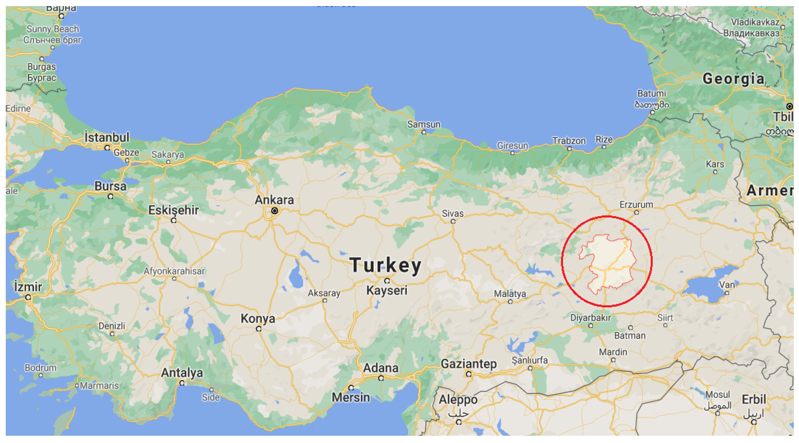
Data taken for this study were collected retrospectively from the archival material of the SERU (Structural Engineering Research Unit) database [50], which was collected from the observational survey by a team of researchers from the Middle East Technical University (METU), Ankara, Turkey. The structural data used in this research is from Bingöl survey that were collected immediately after the Bingöl earthquake, specifically on 1st May 2003 [51]. From that survey, the damage data of 28 reinforced concrete buildings had been selected for this research. The buildings consist primarily of 1 to 6 floors and were designed from the time-span 1970 to 2001. The data consist of various parameters such as irregularities, number of stories, openings, and so forth, verified by the available real images. All irregularities are identified by numbers “1” and “0” that stands for “YES” and “NO”, respectively. The present condition of buildings indicated by “0”, “1”, and “2” to represent “good”, “moderate”, and “poor”, accordingly [51]. Damage states of structures provided in the data are written as “collapse”, “severe”, “moderate”, “light”, and “none” to show the structural damage as well as infill damage, which were merged as a single damage grade as per EMS 98 [46]. Instead of numbers, grades are considered for EMS 98, shown in

Table 14. EMS 98 damage grades as numbers.

EMS 98 Damage Grade	Damage Grade Number
Grade 1	5
Grade 2	4
Grade 3	3
Grade 4	2
Grade 5	1

. Figure 1 represents the location of Bingöl.

As per the data, “No” has been written specifically for the absence of irregularities and buildings without a year of construction and assumed as it has been constructed after 1940. Bingöl falls into a high seismic zone, which has a probability of 10 percent per 50 years, and PGA as 0.556 g (NS) and 0.28 g (EW) [53]. The velocity of soil Vs 30 for the Bingöl earthquake was 529 m/s with an average Peak Ground Velocity (PGV) of 34.5 cm/s in the longitudinal and 21.9 cm/s in the transverse direction in a very dense soil type [54].

4. Results and Discussion

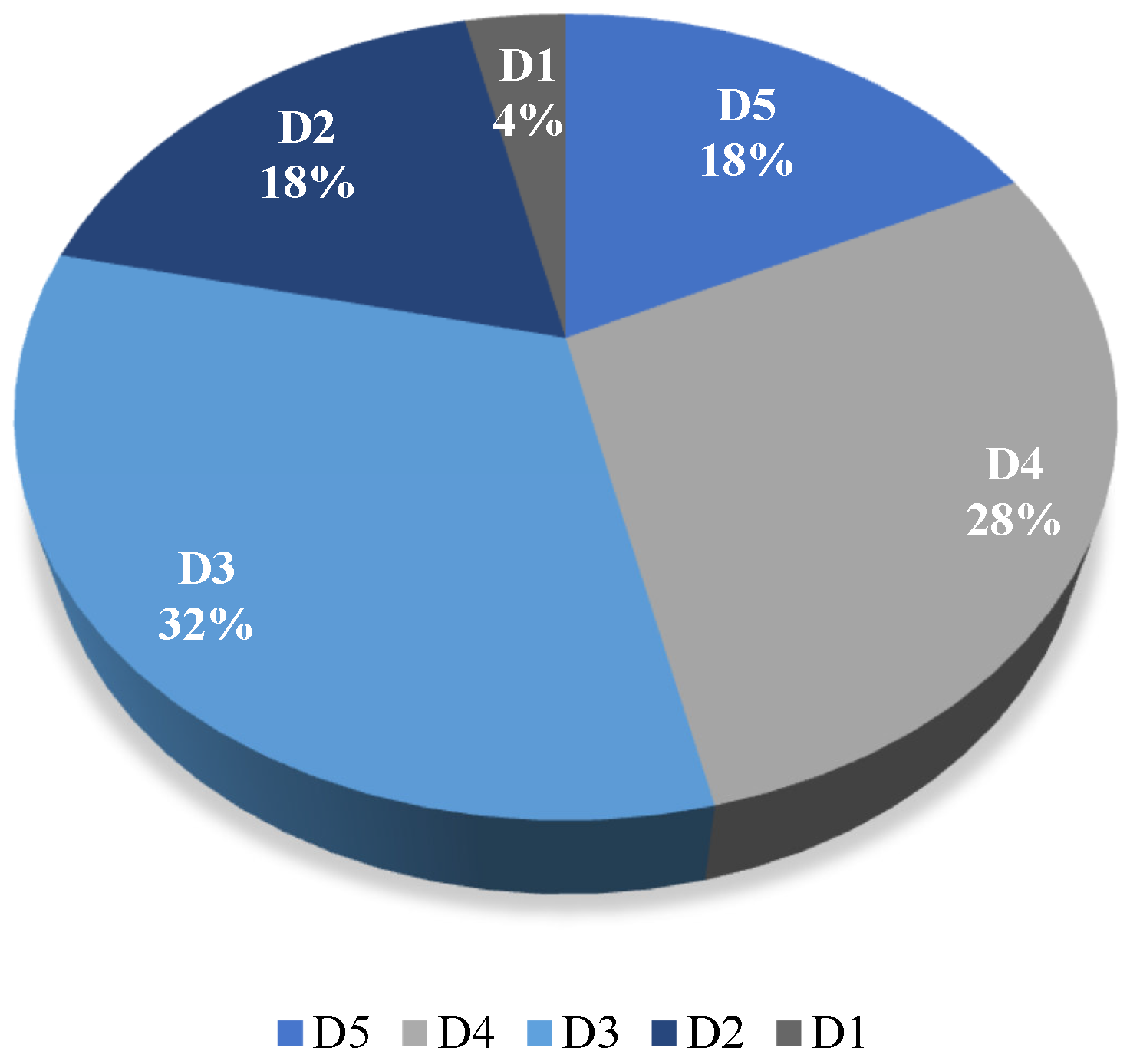
The RVS methodologies based on FEMA P-154, Indian, and Turkish RVS methods have been implemented using the post-earthquake data and then the results were compared with the actual damage occurred to the structures during the Bingöl earthquake. MCDM methods can be validated for multiple earthquake datasets, as each dataset may have variations in the actual damage state of structures. Thus, discovering appropriate MCDM methods and achieving accurate results can help display the damage index. The pie chart in Figure 2 demonstrates the post-earthquake data have divided into 5 proportions according to the actual state of damage. The collected data had been written in terms of words, so to make it easier for interpretation, they have been converted to the numeric form described in the previous section.

Results achieved from various RVS methods have a different scale than the actual damage scale of the data that ranges between 1 to 5. Further, for comparing the results from RVS methodologies to the actual damage, the scale has been converted into 1–5.

Among MCDM methods, a better approach would preferred as per the requirement of the user. In this paper, these requirements were called similarities according to Harirchian et al. [40], where similarity 1 shows the number of buildings indicating exact damage of RVS methodologies to the actual damage. Similarity 2, illustrates the number of buildings through indicating exact damage with the actual damage and number of building with the one-step severe damage. Similarity 3, presents exact damage with the actual damage and number of building with the one-step lighter damage. Whereas, Similarity 4, express the number of buildings in RVS methodologies with exact damage and buildings with any severe damage state. The last similarity indicates the number of buildings in similarity 4 and the number of buildings with one step lighter damage. More detailed information and description of the similarities can be find by Harirchian et al. [40].

In conclusion, similarity 1 is quite identical, and in real scenarios, results may not always be so identical. In the case of a detailed analysis, the priority is safety, then similarity 4 is considered irrespective of time and cost. Further, similarity 2 and 3 gives the damage pretty close to the actual damage. Similarity 5 is performed for the structure that is out of range or slightly affected by the real loss. In general, it becomes riskier when an inappropriate method has been selected for an improper grade. For example, a highly damaged structure has been estimated as slight damage. Therefore, the method with the Turkish code would be more preferable among three RVS methodologies and the one performed with similarities, as Turkish RVS give closer results with the Indian RVS.

The ranking should be specified for all parameters, which are required to perform MCDM methods as shown in

Table 15. Ranking of parameters based on the comparison of methods for ranks scaled from 1 to 9.

Parameters Considered in MCDM	Indian RVS Ranking	FEMA P-154 Ranking	Turkish RVS Ranking	Average Rank	Ranking on [1 to 9 Scale]
Seismic zone	1	1	1	1	9
Building type	1	1		1.5	8
Vertical Irregularity	4	5	4.6	4.5	5
Plan Irregularity	6	3.5		5	4
Code/benchmark	3	2		3	6
Soil type	5	3	1	3	6
No. of stories	2	3	1	2	7
Building quality			4	4.5	5

[39]. The average rank resulting from three RVS methods are considered to determine the final ranking.

4.1. Analogy Using Similarities

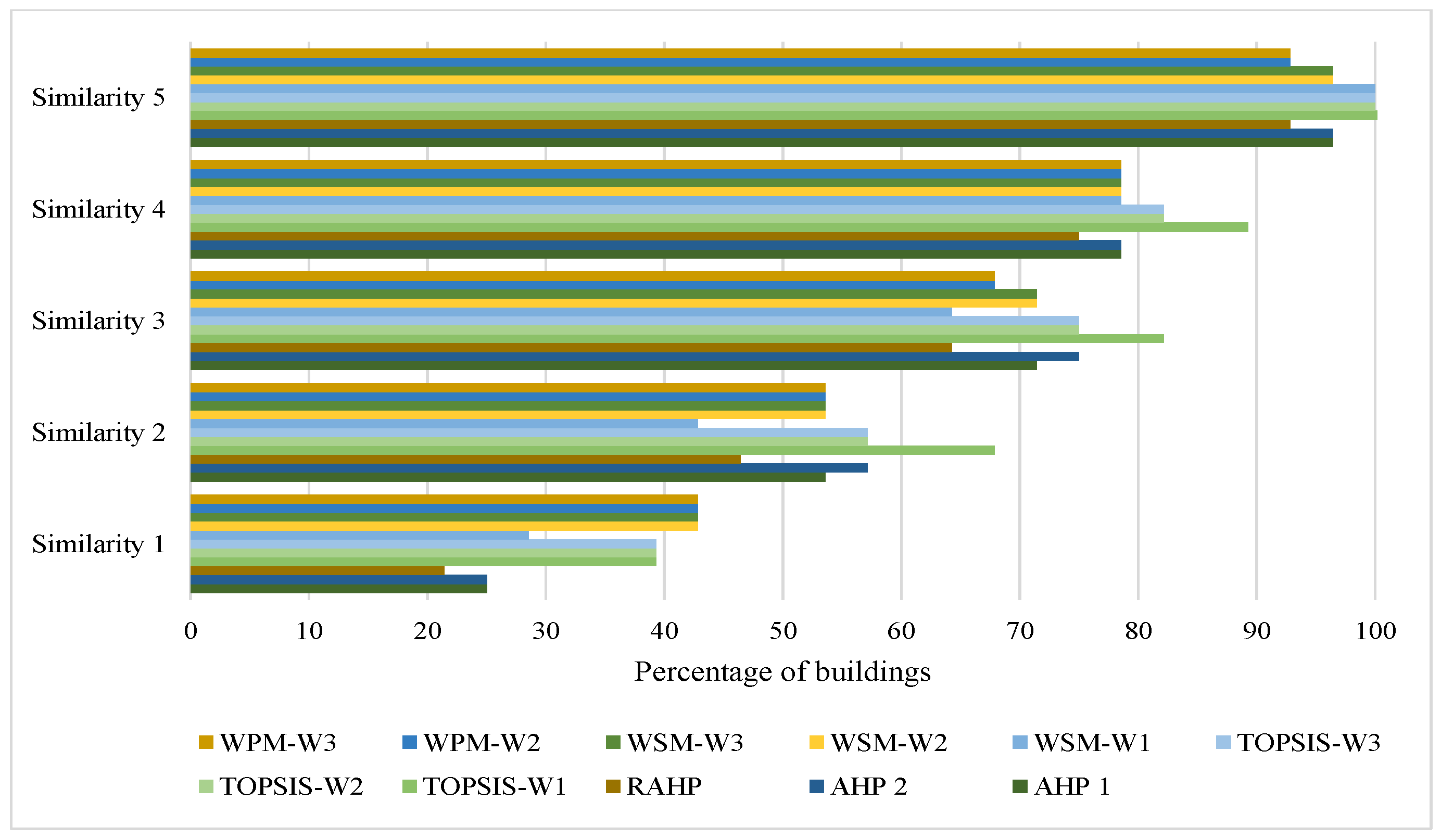
Here is the comparison between damage states of RVS methods to the MCDM methods. Figure 3 represents all 5 similarities used for MCDM methods.

The plot in Figure 3 shows that TOPSIS-W2, W3, WSM-W2, W-3, and WPM-W2, W-3 have contributed to almost exact results. That means normalization of values in the weight calculation process has been done either taking the sum of all numbers or through considering the number. It could not affect TOPSIS, WSM, and WPM, but it has influenced RAHP. Figure 3 shows, for similarity 1, WSM-W2, W3, and WPM-W2, W-3 have provided better results as they have captured almost 36 percent of buildings similar to exact damage, which is followed by TOPSIS with around 33 percent. The rest of the methods gave less than 20 percent of buildings. Theoretically, expectations from RAHP were higher to provide good results compared to AHP 1 and 2, but in this case, the results were opposite. TOPSIS-W1 performed better than TOPSIS-W2, W3, plus it has the best result compared to the rest of the methods for the case of similarities 2, 3, 4, and 5 which is followed by TOPSIS-W2, W3. Moreover, AHP 2 has provided good results after TOPSIS, while in similarities 2 and 3 AHP 2 and TOPSIS-W2, W3 gave the same results.

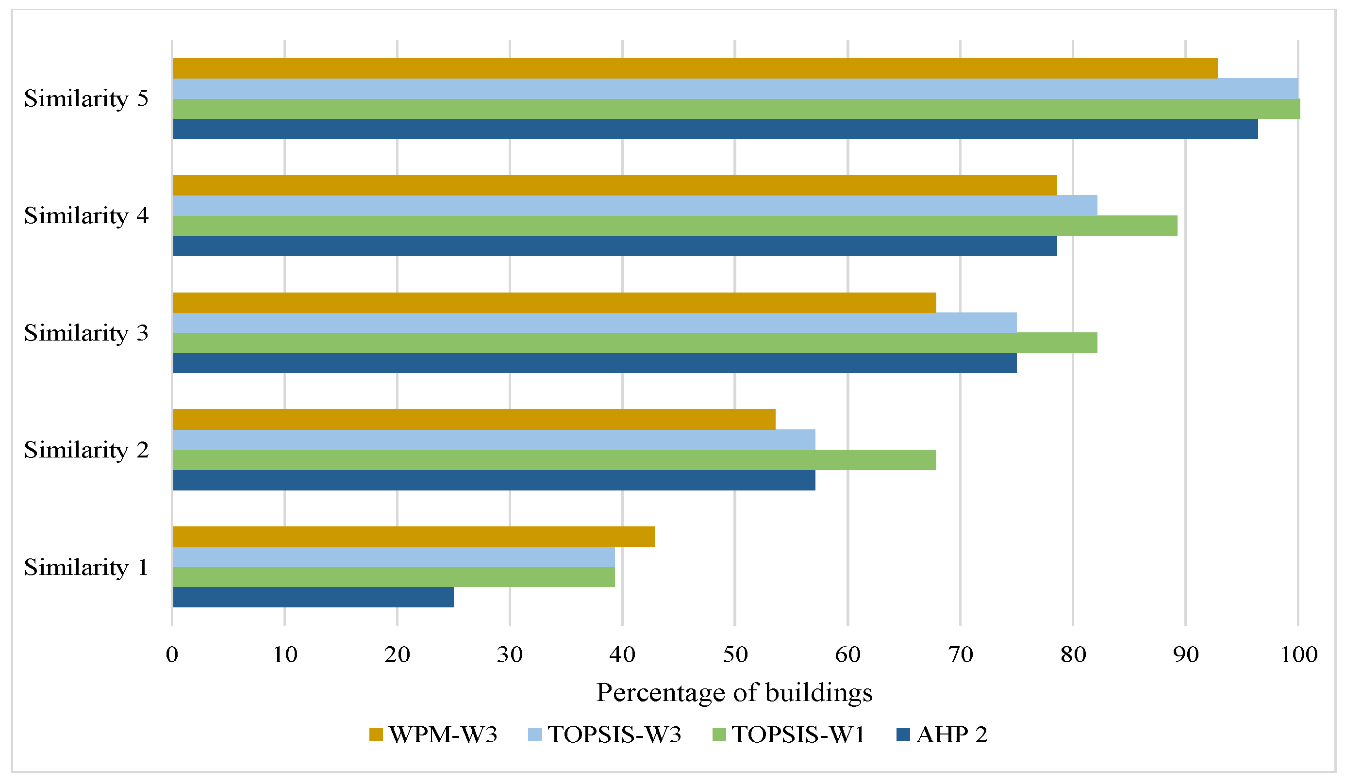
Consequently, the bar chat shows that the TOPSIS-W1 method was better than other methods except in similarity 1; otherwise, WSM-W2, W3, and WPM-W2, W3 could be better. AHP 2 and TOPSIS-W2, W3 were also better methods after the previous ones for similarities 2 and 3. Hence, TOPSIS-W1, W2, AHP 2, and WSM-W2 have been compared further with RVS methodologies. The following Figure 4 shows the comparison of results from the real damage state and proposed RVS based on MCDM methods.

Among MCDM methods, WSM-W2, W3, and WPM-W2, W3 have contributed better results. In the case of other similarities, TOPSIS-W1 gave better results than other MCDM methods. Furthermore, in Figure 5, the comparison of all MCDM methods with the actual damage has been shown. Figure 5 indicated that, for the MCDM methods, TOPSIS-W1 and RAHP have an estimated larger group of buildings which are closer to the actual damage, which includes damage grades 1 and 2 for the output. After that, the results of TOPSIS-W2, W3, and WSM-W2, W3 methods were close to the actual damage, but to compare it with the previous methods, the count was quite less. Amidst all the MCDM methods used in this research, TOPSIS-W1 has contributed to better results than RVS methods followed by WSM-W2, W3, and TOPSIS-W2, W3. In consideration of the WSM-W2, W3, and TOPSIS-W2, W3 performed as second better methods.

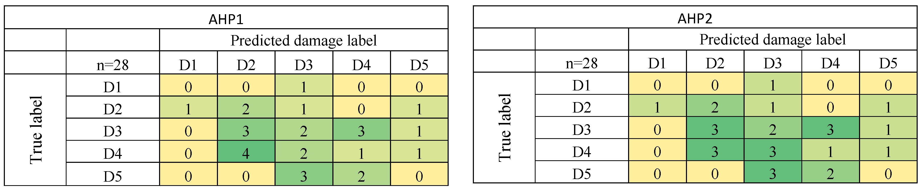
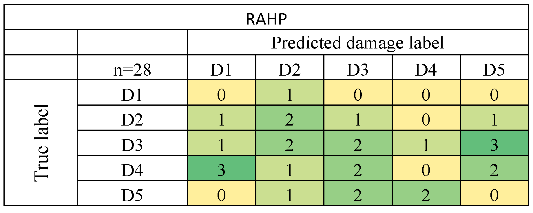
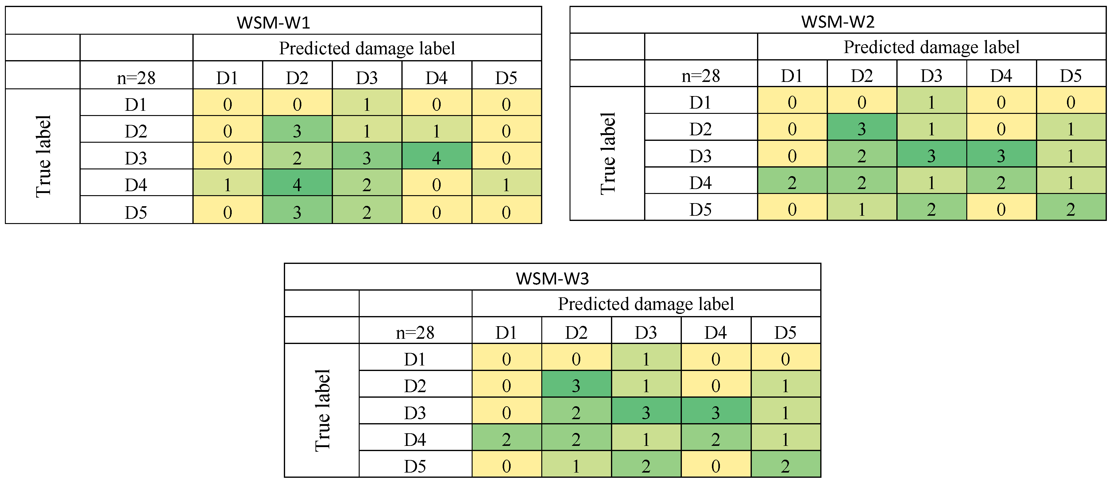
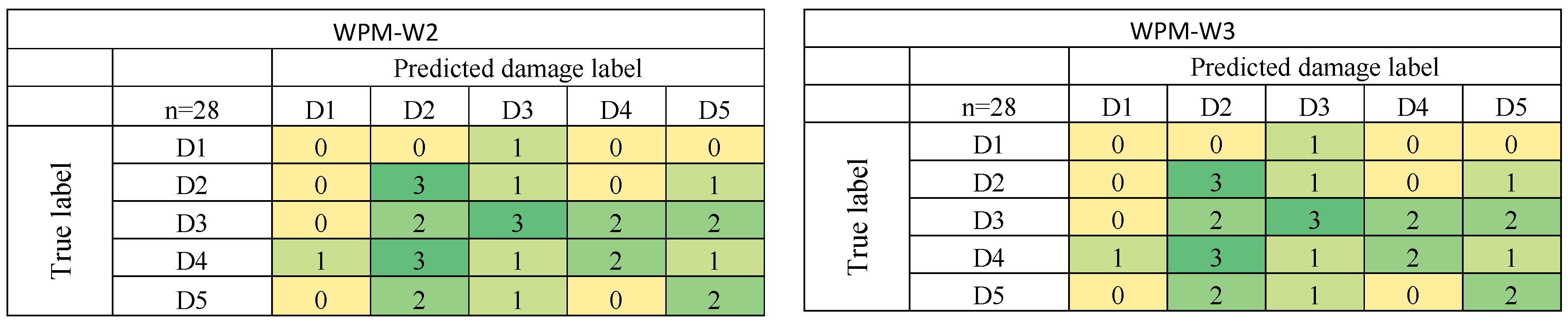
4.2. Analogy Using Confusion Matrices

A confusion matrix, also called an error matrix, represents series of statistics. It helps to envisage the computation for the data to be classified and displayed in the form of matrices. Rows of the matrix demonstrate the prophesied class set as long as columns stand for the real class. The classifier predicts datasets’ occurrence in terms of positive or negative, as it generates four outputs—false positives, false negatives, true positives, and true negatives. In confusion matrices, diagonally placed digits portray a precise range of the predicted class based on the model classifier.

Here it can be seen that in confusion matrices, the damage level has been categorized in 5 damage labels that is, from D1 to D5. The size of the matrix is specified by the number of classes that is, each matrix with [5 × 5] dimensions. Where the X-axis shows the predicted damage label, and Y-axis shows the actual damage. Numerals placed in the confusion matrix signify the damage intensity from 0 to 5 in accordance with EMS 98, shown in Table 14.

Figure 6, Figure 7, Figure 8, Figure 9 and Figure 10 present the confusion matrix of each applied MCDM method in this study. As can be seen, the AHP method had the worst classification while WPM and WSM methods had better damage classifications and distribution of classes.

Table 16. Percentage of accuracy achieved from confusion matrices.

MCDM Methods	Accuracy
AHP1	17.86
AHP2	17.86
RAHP	14.29
TOPSIS-W1	32.14
TOPSIS-W2	32.14
TOPSIS-W3	32.14
WSM-W1	21.43
WSM-W2	35.71
WSM-W3	35.71
WPM-W2	35.71
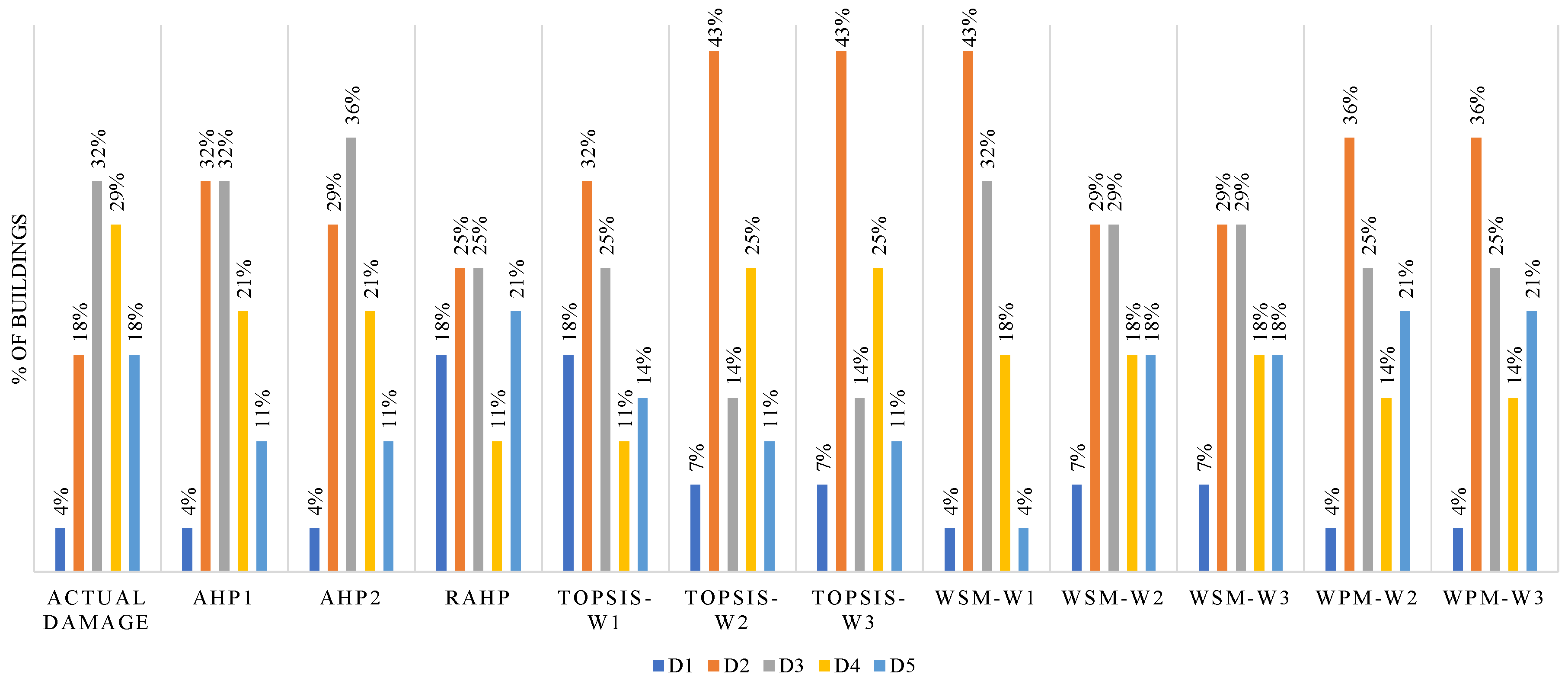
WPM-W3	35.71

demonstrates a better representation of confusion matrices by revealing the accuracy of each method.

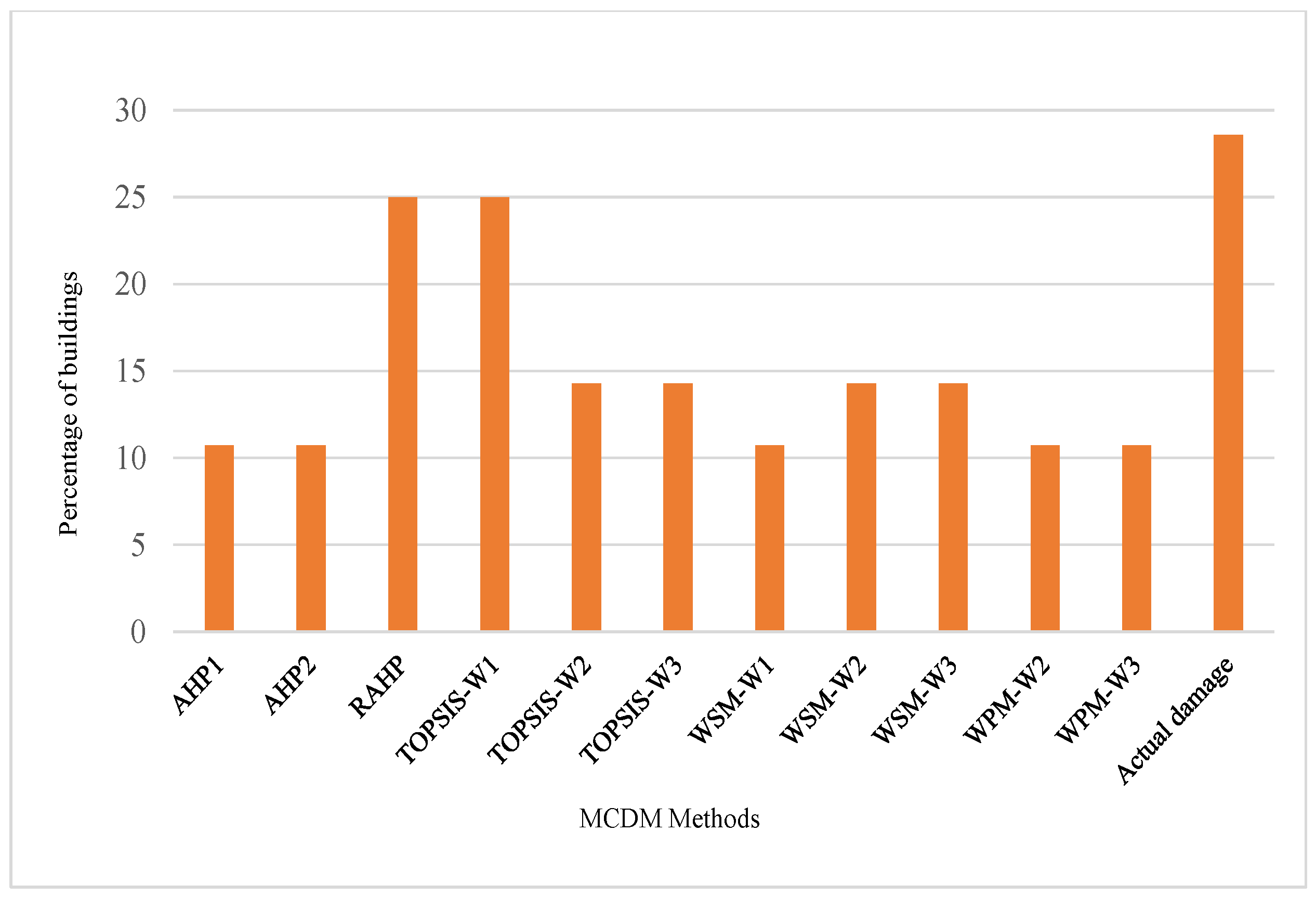
Accuracy is determined with the number of correct predictions among all provided data. In confusion matrices, the overall accuracy depends on the dataset’s consistency, where the number of observations differs according to classes. Therefore, the higher numbers lie in diagonal series show better accuracy of the matrix. Figure 11 shows the percentage of damage distribution in each group between observed actual damages and assessments by different methods. Amid all MCDM methods, the highest accuracy achieved with the WSM and WPM followed by TOPSIS approach.

5. Conclusions

To summarize, it can be observed that the selected MCDM methods are reliable for RVS. In this study, the data of 28 reinforced concrete buildings have been collected from the walk-down survey conducted by the METU team in Bingöl, Turkey, after the Bingöl earthquake in 2003. Furthermore, MCDM methods have been implemented to determine the damage grades for the given post-earthquake building data. Firstly, the validation of the damage index from the MCDM methods and the actual damage state of structures during the Bingöl earthquake have been accomplished. After that, the comparison of the actual damage state, and damage index from the MCDM methods based on three different RVS methods have been executed. From the analogical study, it can be concluded that the MCDM method TOPSIS-W1 contributes more relevant results than rest MCDM methods performed in RVS of structures. The MCDM methods performed in this research have been enlisted in

Table 17. Ranking of MCDM methods used based on results.

MCDM Method	Ranking
TOPSIS-W1	1
RAHP	2
TOPSIS-W2 & W3	3
WSM-W2 & W3	4
AHP 1 & 2, WPM-W2 & W3	5
WSM-W1	6

with descending order based on the obtained results.

In the discussion of executed MCDM methods, TOPSIS-W1 has achieved the top rank. On the second rank, RAHP has been observed but only in case of safety factor because where the similarities were considered, RAHP had the least rank. The outputs of TOPSIS-W2 and W3 were closer when compared to the actual damage than the output of WSM-W2 and W-3, which can be observed from the similarity plot. So, WSM-W2 and W3 were ranked after TOPSIS-W2 and W3. Further, AHP 1, AHP 2, WPM-W2, and W-3 have provided similar plots, so they are one the same rank and listed after methods WSM-W2 and -W3. The reason for their lower ranks is that they had analyzed a smaller number of buildings in damage state 1 compared to WSM-W2, and W-3 methods. In the end, WSM-W1 stands on the last rank due to the lower building application in damage state 1. Also observed in similarities 2 and 3, the results are pretty close to the actual damage state of the structures. The ranking of the methods could not affect the variation in the distribution of parameters.

It can be noticed that the results may differ with the larger amount of data set. Therefore, for future works, the results can be improved according to the varied rate of buildings through performing MCDM methods. For future actions, the complex MCDM methods such as PROMOTHEE, ELECTRE, and many hybrid methods can help identify a more accurate way for this research problem. Moreover, the MCDM methods’ reliability can be checked with other vulnerability cases, which may involve the damage assessment of structures and seismic prioritization based on the seismic vulnerability of the affected regions.