Stationary Target Identification in a Traffic Monitoring Radar System

Abstract

Recently, as one of the intelligent transportation systems, radar systems that monitor traffic on the road have received attention. To ensure the reliable detection performance of the traffic monitoring radar, it is necessary to distinguish stationary road structures from moving vehicles. Therefore, in this paper, we propose a method for discriminating stationary targets in traffic monitoring radar systems. First, we install a frequency-modulated continuous wave radar system using a center frequency of 24.15 GHz on an overpass to monitor multiple lanes on the road. Then, we process the raw data obtained by the radar sensor to extract target information such as the distance, angle, velocity, and radar cross-section. Finally, we analyze the target characteristics in the angle-velocity domain to classify stationary targets and moving vehicles. In this domain, stationary targets appear as points lying around a straight line, and if we estimate that line, we can extract the stationary targets among all targets. To find the trend line, we use a random sample consensus-based estimation method, which can extract a dominant line component from a set of sample points. Through the proposed method, we can effectively remove the stationary targets in the field of view of the radar system.

1. Introduction

To realize autonomous driving, an autonomous vehicle must be equipped with automotive sensors such as cameras, LiDARs, and radars. In recent years, the development of autonomous driving technology has been accelerating due to advances in sensors for vehicles. For autonomous driving, not only the development of automotive sensors, but also the construction of intelligent road infrastructure is necessary. One of the essential factors for building an intelligent transportation system (ITS) is to monitor the volume and flow of vehicles on the road, which is known as traffic management. If the road traffic information can be measured and delivered to each driver on the road, more efficient road management will be possible. In other words, by analyzing traffic conditions in real time, it is possible to manage road traffic efficiently and implement optimal signaling systems In addition, the ITS can help drivers choose efficient routes and shorten the time to reach their destination.

The most frequently used system for the measurement of road traffic is a camera-based monitoring system [1,2]. For instance, a high-definition camera-based ITS with wireless communications was proposed for traffic surveillance in [3]. Recently, several studies have been conducted to use radar sensors for road traffic monitoring in addition to the camera-based surveillance systems. For example, the Global System for Mobile Communication (GSM)-based passive radar to monitor the road traffic was introduced in [4,5]. They suggested the possibility of using the GSM-based radar to detect the velocity of the vehicle. In [6], the authors presented a method for estimating the range, velocity, and angle information of vehicles using a 35 GHz interferometric traffic monitoring radar system. In addition, the feasibility of road surveillance using passive radar systems was suggested in [7]. Recently, a method for identifying multiple lanes by clustering detection points in each lane in a frequency-shift keying radar system was proposed in [8].

These radar-based road monitoring systems can compensate for the weaknesses of the camera-based road surveillance systems. For example, in the case of the camera-based method, the detection performance is severely deteriorated in a lightless environment. In addition, the camera-based methods have the disadvantage of being vulnerable in terms of privacy protection. On the other hand, if radar is used for road monitoring, it is also effective in terms of personal privacy protection because it does not take a picture of the driver. Moreover, using the intrinsic function of radar, estimating the distance to the target and the velocity of the target, we can also get more information than we can get with the camera sensor. For example, the velocity of the vehicle can be measured directly using radar, which can replace the speedometer. In addition, counting the number of vehicles passing through a specific section is also one of the functions that can be easily implemented with radar.

In general, traffic monitoring radars are installed at specific points on viaducts or bridges to face multiple lanes, as shown in Figure 1.

In this environment, the traffic monitoring radar continuously receives radar signals reflected from road structures, such as guardrails and median strips. Because these structures are usually made of steel, they strongly reflect radar signals, and the radar perceives them as meaningful targets. Some studies on the adverse effects of the presence of these road structures on the radar detection performance were presented in [9,10,11]. If such misinformation is transmitted to a driver on the road through ITS, this can lead to a dangerous situation for the driver. Therefore, a signal processing that allows the radar to recognize road structures by itself should be applied. The significant difference between road structures and vehicles is that the structures are fixed to the road. Thus, we propose a method for discriminating stationary road structures and moving vehicles using the velocity characteristics of the detected targets, which makes the detection performance of the traffic monitoring radar reliable. The authors in [12] proposed a method to classify moving targets and stationary targets in the time-frequency domain. However, in this method, it is impossible to immediately classify the target because the data accumulated in the time axis are used. In other words, the method in [12] cannot be applied in real time.

In our work, the target characteristics in the angle-velocity domain are used to classify stationary structures and moving vehicles. Unlike moving targets, stationary targets have a certain tendency in this domain, which means stationary targets appear as sample points on a line. Thus, if the straight line can be estimated, we can only extract stationary targets. To estimate the trend line, we use the M-estimator sample and consensus (MSAC) algorithm [13], which is a more advanced algorithm from random sample consensus (RANSAC) [14,15]. The RANSAC and MSAC algorithms can extract points with a certain trend from multiple sample points. Using the data measured on the highway, we evaluate the performance of the proposed classification method and compare it with the conventional method such as linear regression. Through the proposed method, it is possible to classify meaningful targets among a number of detected targets at every signal processing cycle, unlike the method in [12]. In addition, our proposed method shows stable and reliable performance because it does not classify the targets using a simple threshold value, but classifies them by finding a trend in the measured data.

The remainder of this paper is organized as follows. In Section 2, we introduce our traffic monitoring radar and basic signal processing used for target detection in the radar system. Then, the signal measurement environment and target detection results using our radar sensor are described in Section 3. Next, in Section 4, the proposed stationary target identification method and its classification performance are presented. Finally, we conclude this paper in Section 5.

2. Traffic Monitoring Radar System

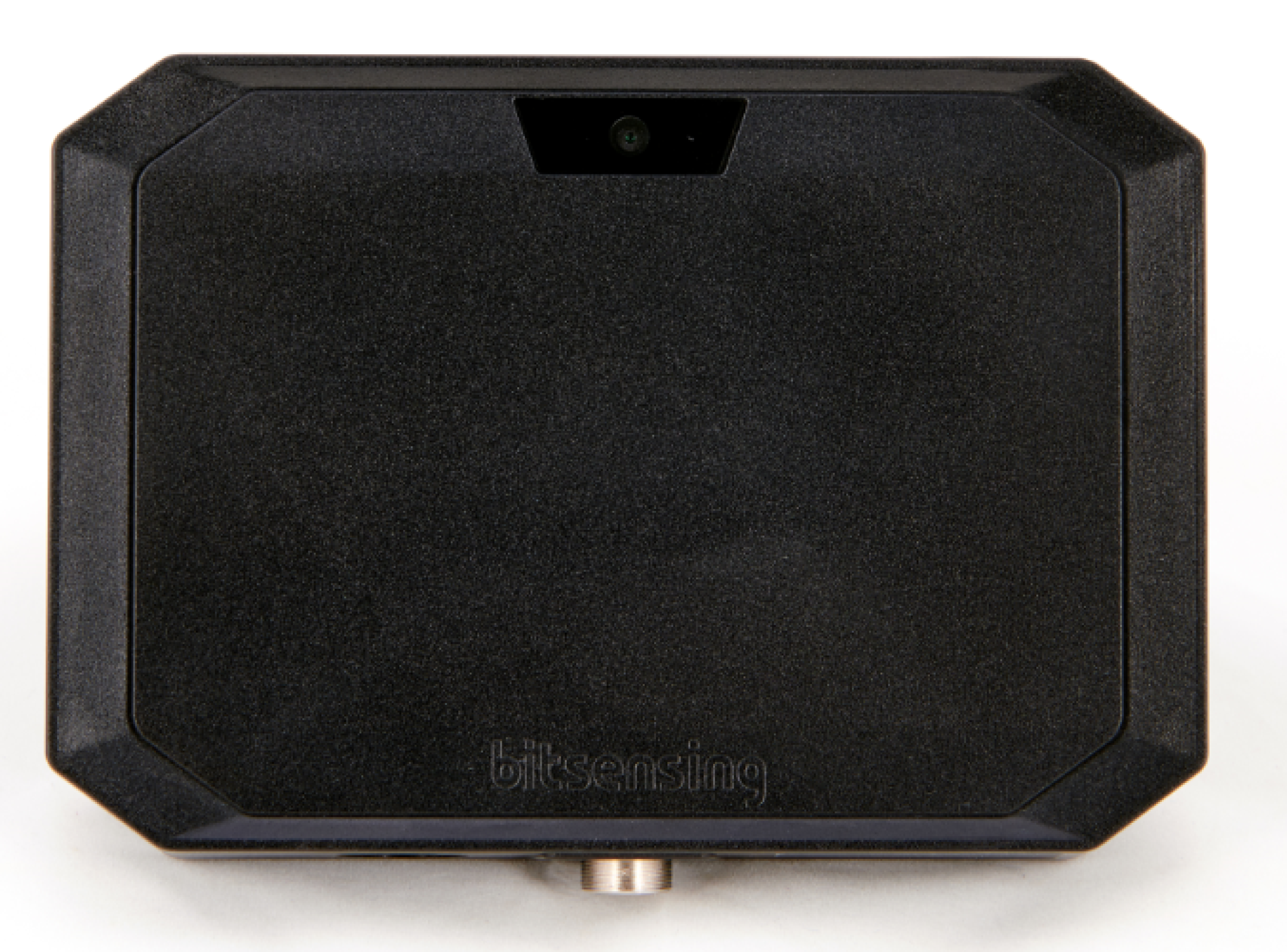
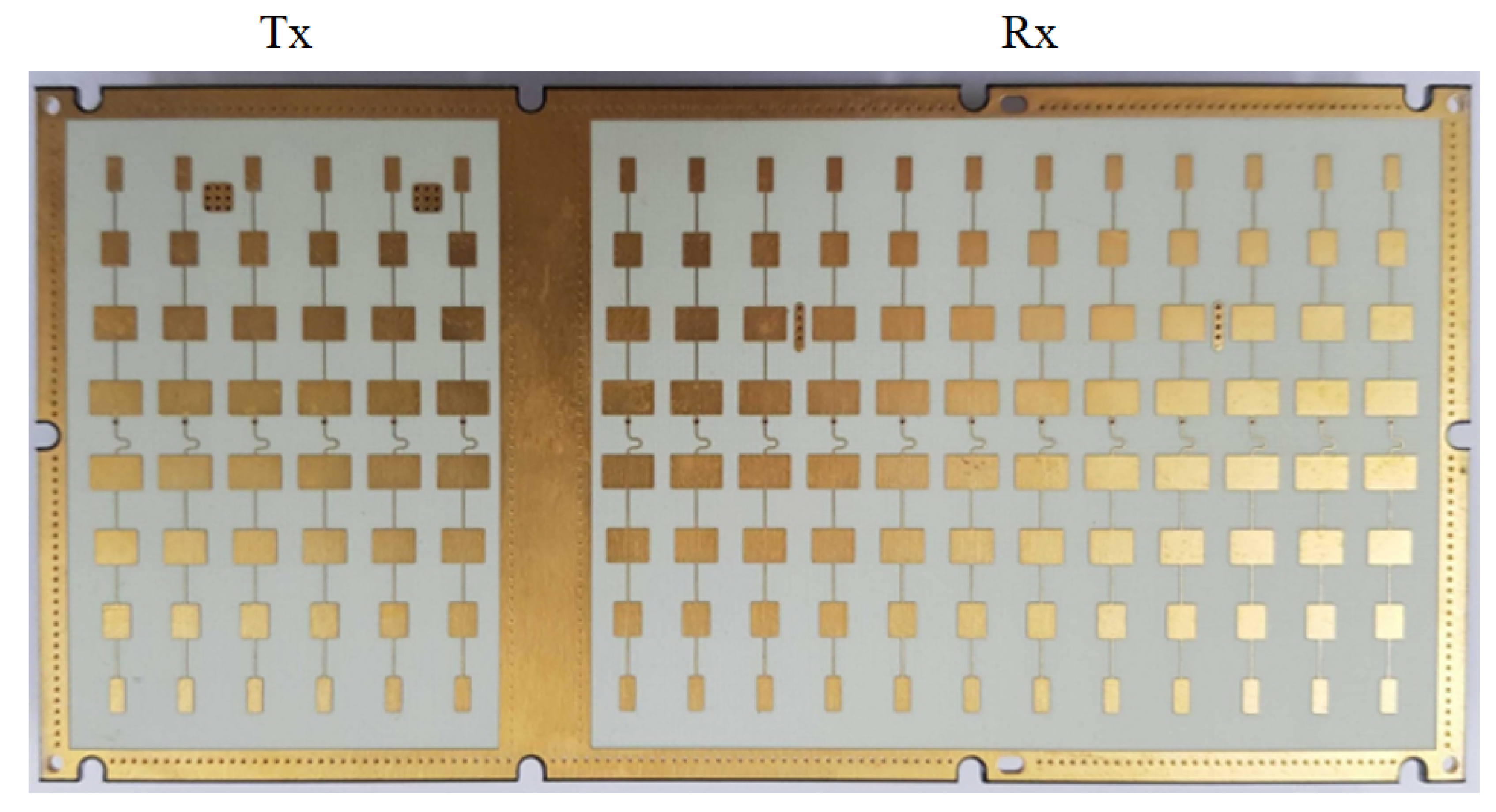
2.1. Traffic Monitoring Radar

In this work, we use a frequency-modulated continuous wave (FMCW) radar that we have developed [16] to monitor road traffic, which is shown in Figure 2.

This FMCW radar uses a frequency band of 24.05 to 24.25 GHz (i.e., an operating bandwidth of 200 MHz), so the range resolution reaches tens of centimeters. The radar we designed uses a single transmit antenna element and an array antenna system with multiple receiving antenna elements (e.g., four antenna elements), as shown in Figure 3.

As the antenna system, a series-fed patch array antenna is used, and the antenna spacing between the receiving antenna elements is $\frac{3c}{2f_c}$, where $f_c$ and c denote the center frequency of the radar signal and the speed of light. Based on the antenna system of the radar, it can detect vehicles driving in four different lanes.

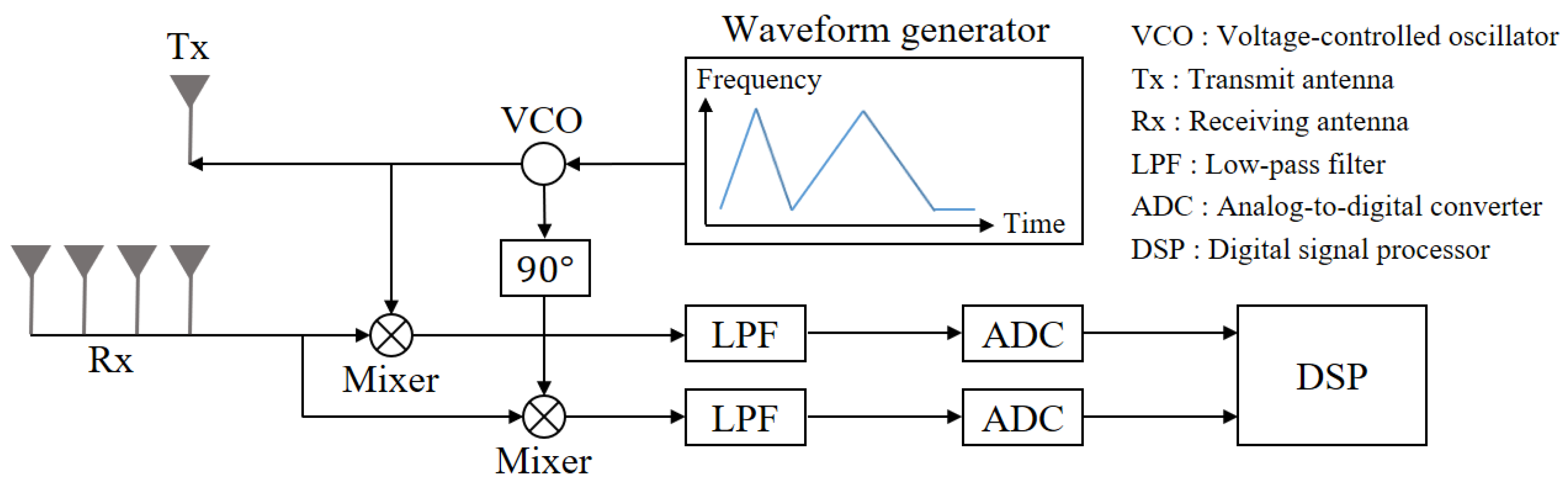
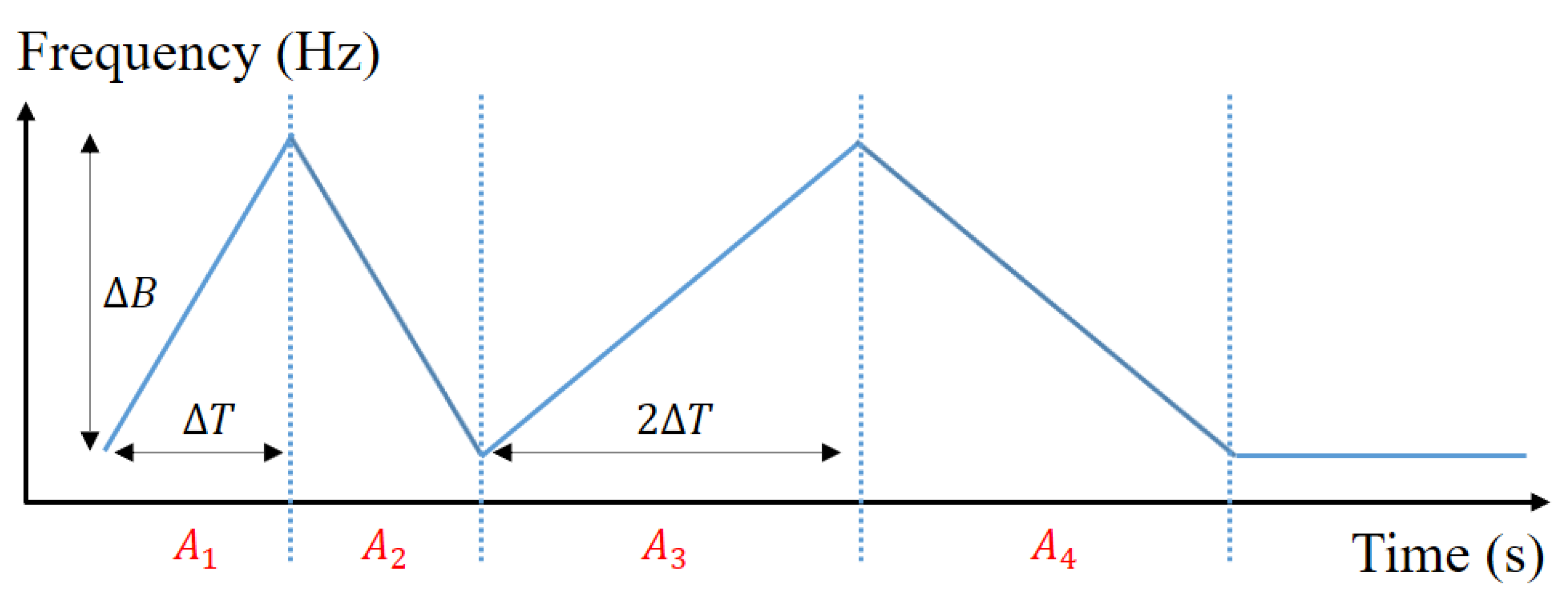
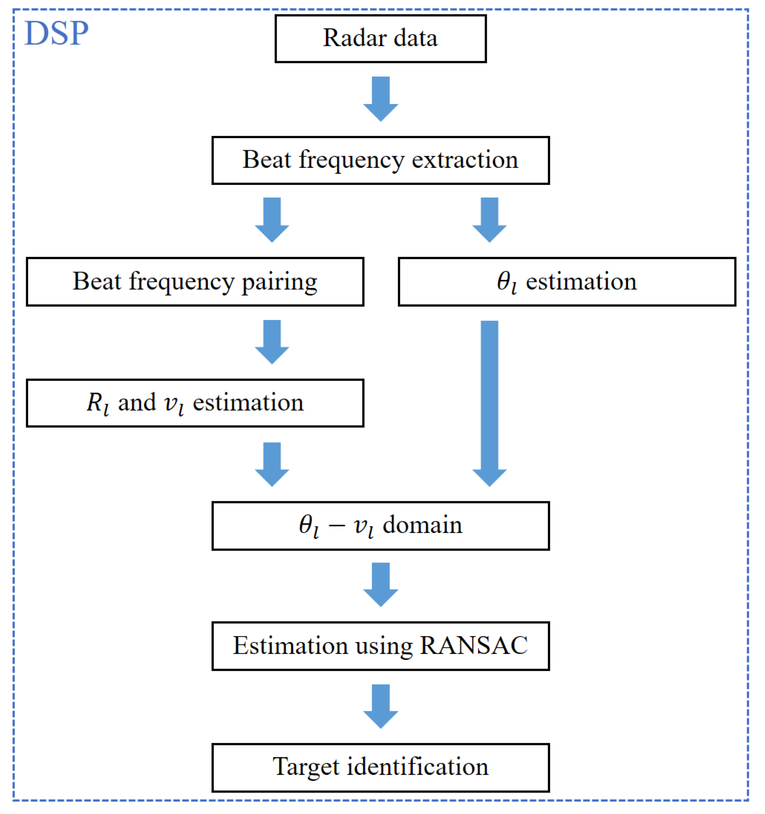
2.2. Radar Signal Processing for Target Information Extraction

In this section, we describe the signal processing technique used in our traffic monitoring radar system. The schematic block diagram of our radar system is depicted in Figure 4.

In this block diagram, the radar system consists of the waveform generator, voltage-controlled oscillator (VCO), transmit antenna element (Tx), four receiving antenna elements (Rx), frequency mixer, low-pass filter (LPF), analog-to-digital converter (ADC), and digital signal processor (DSP).

First, in the FMCW radar system, a waveform whose frequency changes linearly with time is made from the waveform generator. The detailed frequency change pattern of the waveform over time is shown in Figure 5.

As shown in the figure, the frequency-modulated waveform can be divided into four areas (i.e., $A_1$, $A_2$, $A_3$, and $A_4$) according to the change of time. In $A_1$, the transmitted waveform can be expressed as:

$$s_t^{\left(1\right)}\left(t\right)={\alpha }_t\cos \left(2\pi \right(f_c-\frac{\Delta B}{2})t+\pi \frac{\Delta B}{\Delta T}{t}^2)(0\le t\le \Delta T),$$

(1)

where ${\alpha }_t$, $\Delta B$, and $\Delta T$ are the amplitude, bandwidth, and sweep time of the transmitted waveform. When $s_t^{\left(1\right)}\left(t\right)$ is transmitted and reflected from L targets, the received signal $s_r^{\left(1\right)}\left(t\right)$ can be expressed as:

$$s_r^{\left(1\right)}\left(t\right)=\sum _{l=1}^L\left\{{\alpha }_{r_l}\cos \right(2\pi (f_c+f_{d_l}-\frac{\Delta B}{2})(t-t_{d_l})+\pi \frac{\Delta B}{\Delta T}{(t-t_{d_l})}^2\left)\right\},$$

(2)

where ${\alpha }_{r_l}(l=1,2,\dots ,L)$ is the amplitude of the received signal reflected from the $l_{th}$ target. In addition, $f_{d_l}$ is the Doppler shift caused by the relative velocity between the radar and the $l_{th}$ target and $t_{d_l}$ is the time delay caused by the relative distance between the radar and the $l_{th}$ target.

Then, $s_t^{\left(1\right)}\left(t\right)$ and $s_r^{\left(1\right)}\left(t\right)$ are multiplied by the frequency mixer and passed through the LPF, as shown in Figure 4. The final output of the filter with high frequency components disappearing can be expressed as:

$$s_L^{\left(1\right)}\left(t\right)=\frac{1}{2}{\alpha }_t\sum _{l=1}^L{\alpha }_{r_l}\cos \left(2\pi \right((\frac{\Delta B}{\Delta T}{t}_{d_l}-f_{d_l})t+(f_c+f_{d_l}-\frac{\Delta B}{2})t_{d_l}-\frac{\Delta B}{2\Delta T}{t_{d_l}}^2\left)\right).$$

(3)

As given by Equation (3), the filter output has the form of a sum of sinusoids with different frequencies. These frequencies contain range and velocity information for each target. Therefore, if the Fourier transform is applied to the time-domain filter output in Equation (3), it is possible to estimate the frequencies containing the distance and velocity information of the target. The frequency estimated from the Fourier transform is given as:

$$\begin{array}{cc}{\hat{f}}_l^{\left(1\right)}& =\frac{\Delta B}{\Delta T}{t}_{d_l}-f_{d_l}\hfill \\ & =\frac{\Delta B}{\Delta T}\frac{2R_l}{c}-\frac{2v_l}{c}{f}_c,\hfill \end{array}$$

(4)

where $R_l$ and $v_l$ are the relative distance and relative velocity between the radar and the $l_{th}$ target. This frequency is also called the beat frequency because it indicates the frequency difference between the transmitted and received waveforms.

However, from Equation (4), $R_l$ and $v_l$ of the $l_{th}$ target are coupled to each other, so they cannot be separated. Therefore, the additional waveform in $A_2$ of Figure 5 is needed. In $A_2$, the transmitted waveform also can be expressed as:

$$s_t^{\left(2\right)}\left(t\right)={\alpha }_t\cos \left(2\pi \right(f_c+\frac{3\Delta B}{2})t-\pi \frac{\Delta B}{\Delta T}{t}^2)(\Delta T\le t\le 2\Delta T).$$

(5)

This waveform also passes through the frequency mixer and the filter, and the filter output can be expressed as:

$$s_L^{\left(2\right)}\left(t\right)=\frac{1}{2}{\alpha }_t\sum _{l=1}^L{\alpha }_{r_l}\cos \left(2\pi \right((\frac{\Delta B}{\Delta T}{t}_{d_l}+f_{d_l})t-(f_c+f_{d_l}+\frac{3\Delta B}{2})t_{d_l}-\frac{\Delta B}{2\Delta T}{t_{d_l}}^2\left)\right).$$

(6)

If we apply the Fourier transform to $s_L^{\left(2\right)}\left(t\right)$, we can estimate a frequency different from Equation (4). The new frequency can be expressed as:

$$\begin{array}{cc}{\widehat{f}}_l^{\left(2\right)}& =\frac{\Delta B}{\Delta T}{t}_{d_l}+f_{d_l}\hfill \\ & =\frac{\Delta B}{\Delta T}\frac{2R_l}{c}+\frac{2v_l}{c}{f}_c.\hfill \end{array}$$

(7)

Therefore, we can finally estimate $R_l$ and $v_l$ using Equations (4) and (7) as follows:

$$R_l=({\widehat{f}}_l^{\left(1\right)}+{\widehat{f}}_l^{\left(2\right)})\times \frac{c\Delta T}{4\Delta B}$$

(8)

and:

$$v_l=({\widehat{f}}_l^{\left(2\right)}-{\widehat{f}}_l^{\left(1\right)})\times \frac{c}{4f_c}.$$

(9)

If multiple targets exist in the field of view (FOV) of the radar, it may be difficult to effectively pair ${\widehat{f}}_l^{\left(1\right)}$ and ${\widehat{f}}_l^{\left(2\right)}$ for the $l_{th}$ target. In other words, ambiguity occurs when pairing multiple beat frequencies [17]. Therefore, we additionally use the waveforms in $A_3$ and $A_4$ [18], shown in Figure 5. The waveforms in $A_3$ and $A_4$ can be expressed as:

$$s_t^{\left(3\right)}\left(t\right)=A_T\cos \left(2\pi \right(f_c-\frac{3\Delta B}{2})t+\pi \frac{\Delta B}{2\Delta T}{t}^2)(2\Delta T\le t\le 4\Delta T)$$

(10)

and:

$$s_t^{\left(4\right)}\left(t\right)=A_T\cos \left(2\pi \right(f_c+\frac{5\Delta B}{2})t-\pi \frac{\Delta B}{2\Delta T}{t}^2)(4\Delta T\le t\le 6\Delta T).$$

(11)

From Equations (10) and (11), two frequencies can be additionally obtained through the same process as processing the signals in $A_1$ and $A_2$. The two new frequencies can be expressed as:

$$\begin{array}{cc}{\widehat{f}}_l^{\left(3\right)}& =\frac{\Delta B}{2\Delta T}{t}_{d_l}-f_{d_l}\hfill \\ & =\frac{\Delta B}{2\Delta T}\frac{2R_l}{c}-\frac{2v_l}{c}{f}_c\hfill \end{array}$$

(12)

and:

$$\begin{array}{cc}{\widehat{f}}_l^{\left(4\right)}& =\frac{\Delta B}{2\Delta T}{t}_{d_l}+f_{d_l}\hfill \\ & =\frac{\Delta B}{2\Delta T}\frac{2R_l}{c}+\frac{2v_l}{c}{f}_c.\hfill \end{array}$$

(13)

Finally, using the four beat frequencies (i.e., ${\widehat{f}}_l^{\left(1\right)},{\widehat{f}}_l^{\left(2\right)},{\widehat{f}}_l^{\left(3\right)}$, and ${\widehat{f}}_l^{\left(4\right)}$), we can effectively estimate the relative distance and relative velocity of each target even in cases where multiple targets exist.

To obtain accurate position information of a target, not only distance information, but also angle information must be accurately estimated. The radar we designed utilizes an array antenna system with four receiving antenna elements, as shown in Figure 3. In the array antenna system, angle information of the $l_{th}$ target, ${\theta }_l$, can be estimated using the phase difference between signals received from each receiving antenna channel [19]. Many estimation algorithms, such as the fast Fourier transform [20], the Bartlett method [21], and the multiple signal classification [22,23], can be used to find the phase difference between the receiving channels. In our radar system, we use the Bartlett algorithm as the angle estimation algorithm. The Bartlett algorithm has the advantage of having good angular resolution while being able to be applied in real time due to its low computational complexity [24].

3. Signal Measurement and Target Detection Using Traffic Monitoring Radar

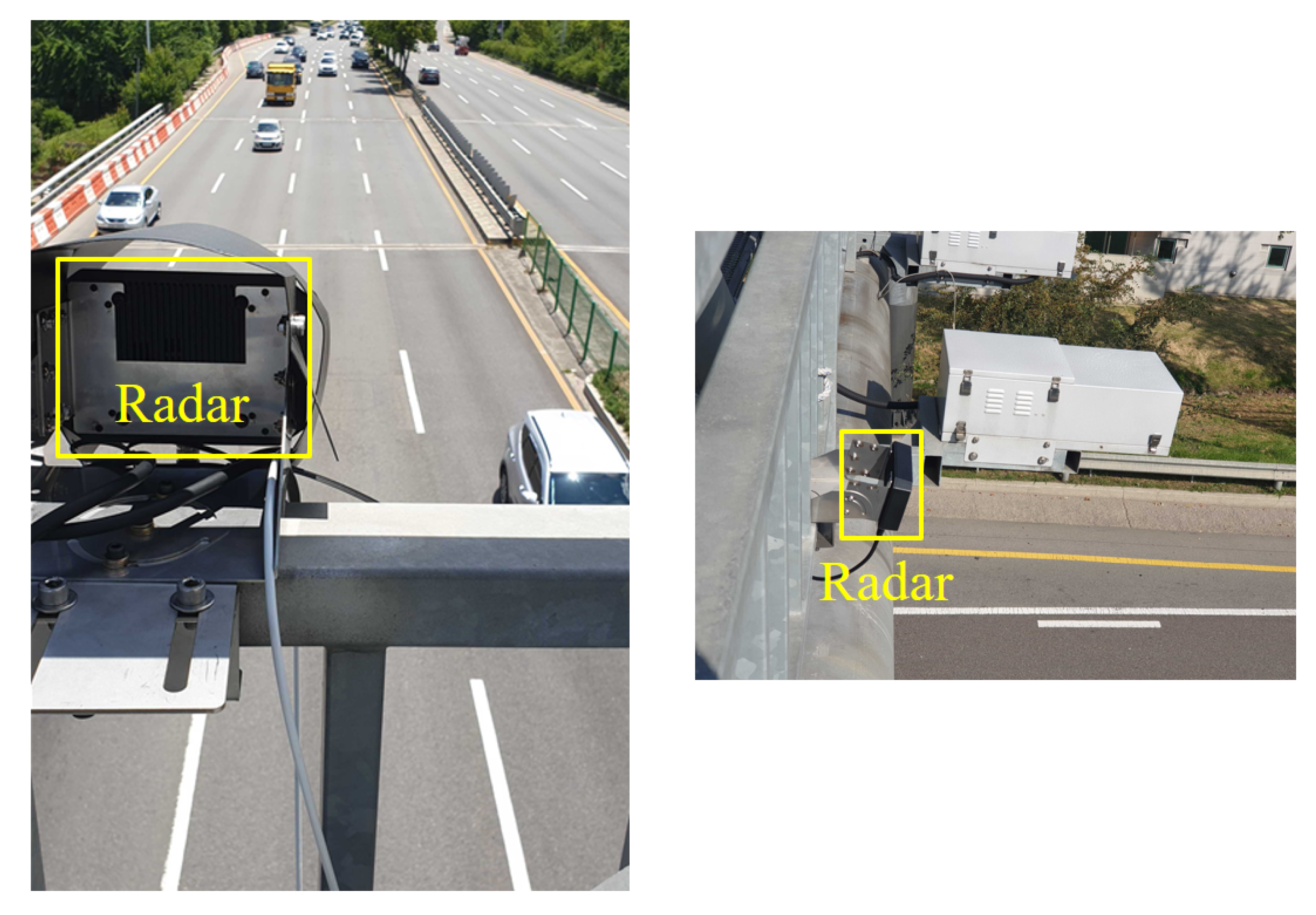
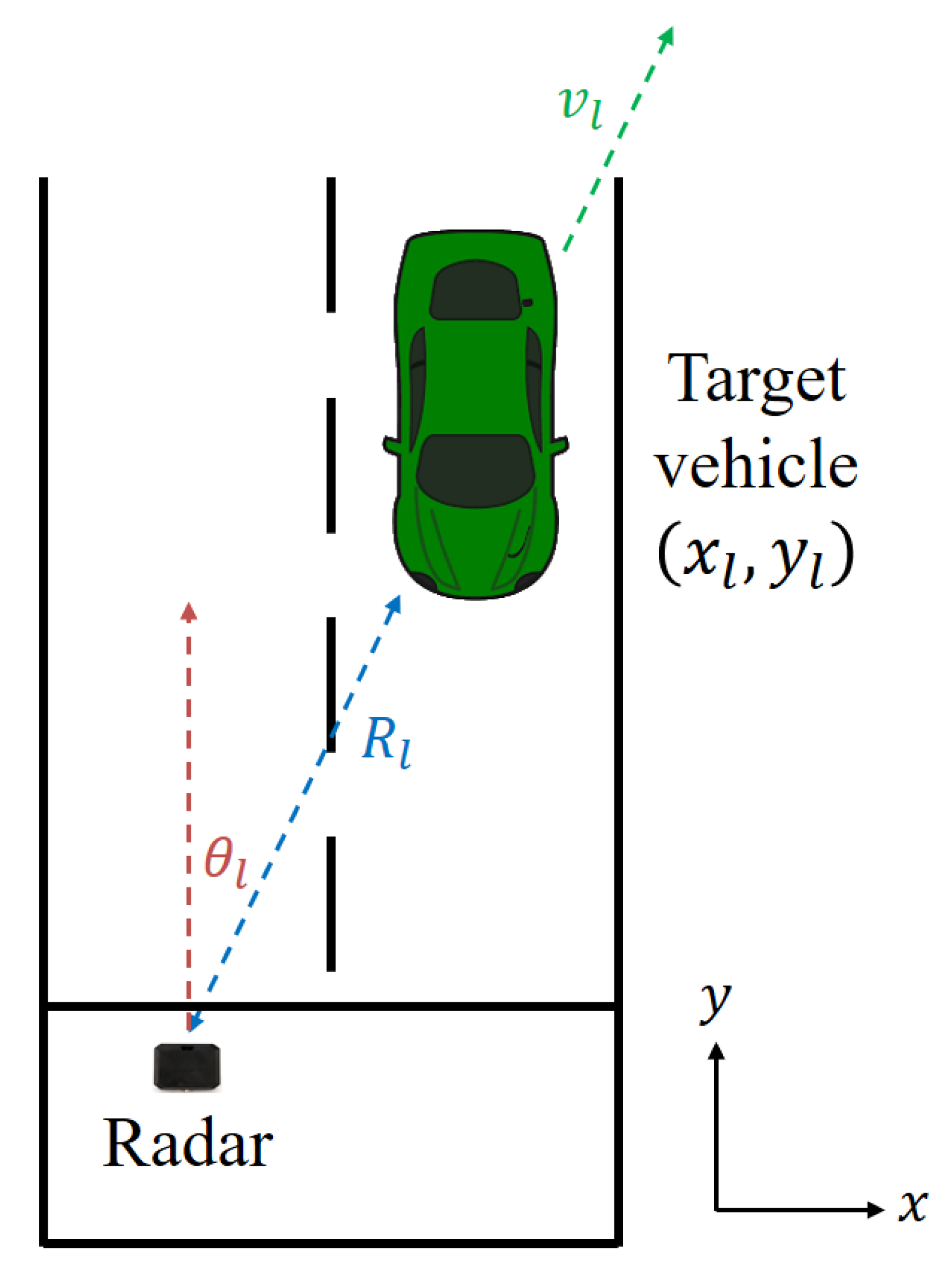
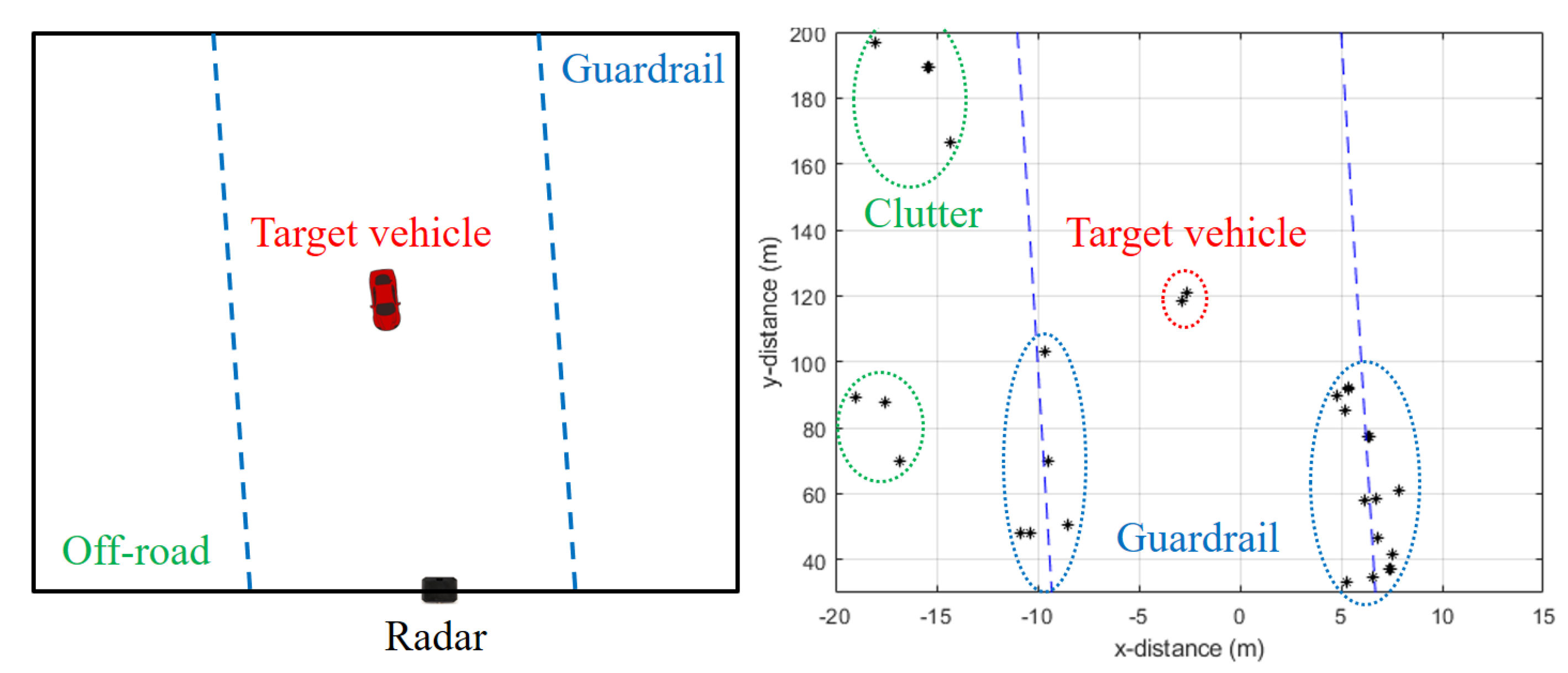
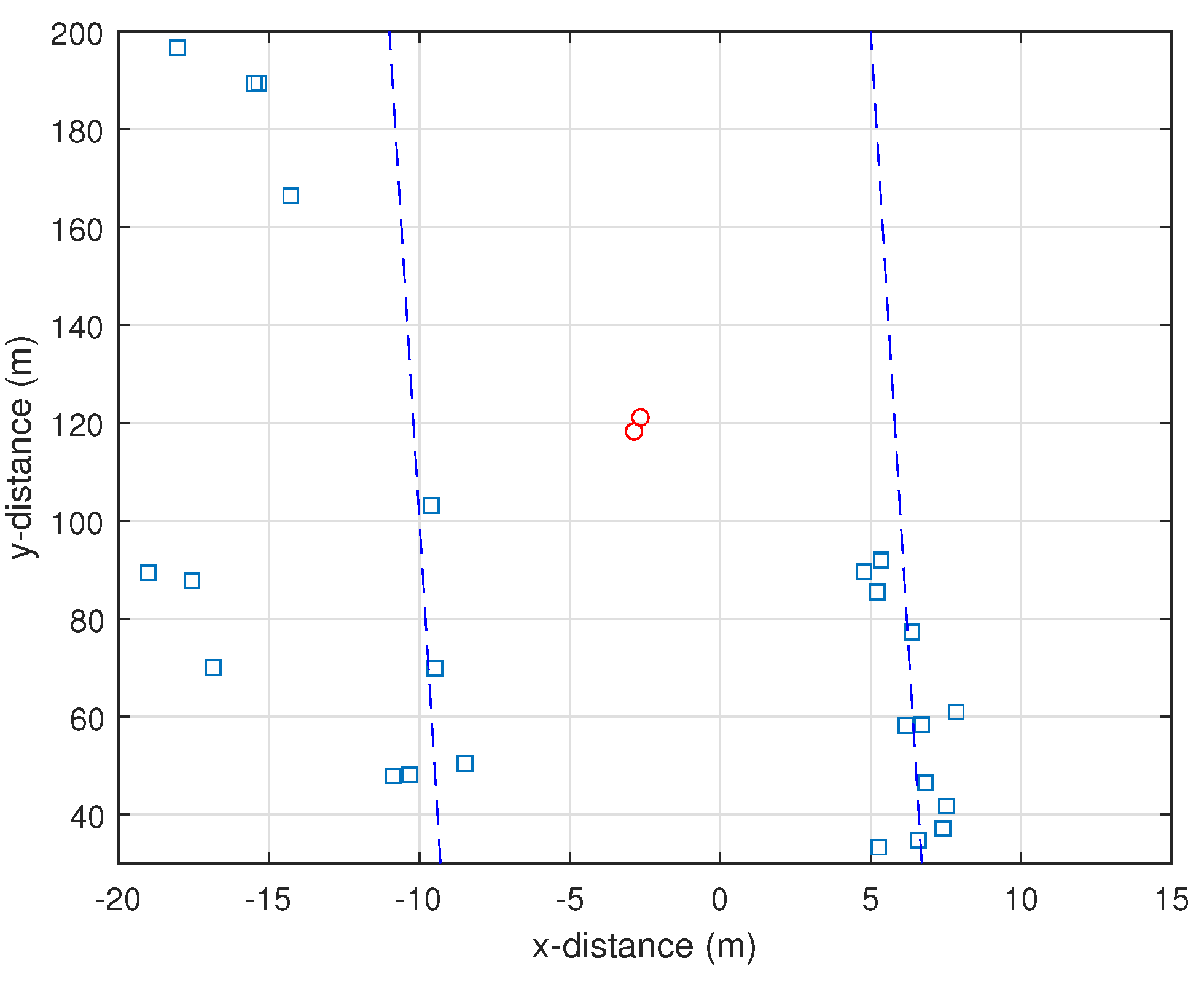
3.1. Measurement Environment

We conducted signal measurements with the radar system described in Section 2. As shown in Figure 1, we installed our radar on an overpass, with the radar facing the highway. The specifications of our radar are given in

Table 1. Specifications of the traffic monitoring radar system.

Parameters of Our Radar System	Parameter Values
Center frequency, $f_c$	24.15 GHz
Bandwidth, $\Delta B$	200 MHz
Detectable range	2 to 300 m
Range resolution	80 cm
Detectable velocity	−250 to 250 km/h
Velocity resolution	1.2 m/s
Field of view	−15$°$ to 15$°$
Frame time	33 ms

.

The radar we designed can detect up to 300 m for up to four lanes, as given in Table 1. Considering the range resolution of 80 cm, vehicles such as trailers will be detected as more points than sedans. In addition, looking at Figure 1, we can expect that not only the vehicles driving on the road, but also structures such as guardrails will be detected because they are within the FOV of the radar.

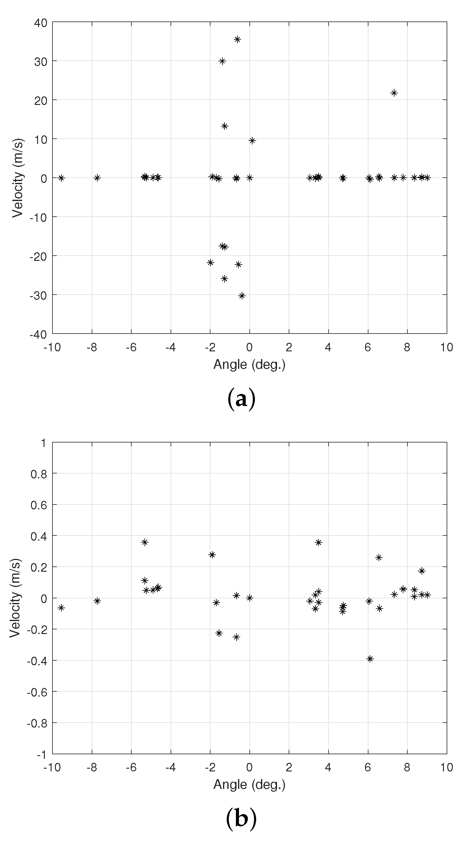
3.2. Detection Results from Radar Signal Processing

Using the signal processing method described in Section 2, the target information, such as $R_l$, $v_l$, and ${\theta }_l$ of the target, can be extracted in our traffic-monitoring radar system. The $R_l$ and $v_l$ information obtained here indicates the range and velocity in the radial direction, as shown in Figure 6.

Thus, using the estimated values of $R_l$ and ${\theta }_l$, we can express the position of the $l_{th}$ target in the Cartesian coordinate system as:

$$(x_l,y_l)=(R_l\sin {\theta }_l,R_l\cos {\theta }_l).$$

(14)

For example, Figure 7 shows the detection result obtained from the traffic monitoring radar installed on the overpass. This figure shows a two-dimensional range map converted to a Cartesian coordinate system using $R_l$ and ${\theta }_l$.

The experimental data were acquired in the same environment as in Figure 1. A vehicle was approaching the radar, and guardrails were located on the left and right sides of the road. There was a forest on the left side of the guardrail. In this road environment, a number of points corresponding to a target vehicle and guardrails on either side of the road are detected. In addition, radar clutter also occurs due to trees in the forest off the road. In this case, if a meaningful moving target can be identified, more stable detection performance can be achieved.

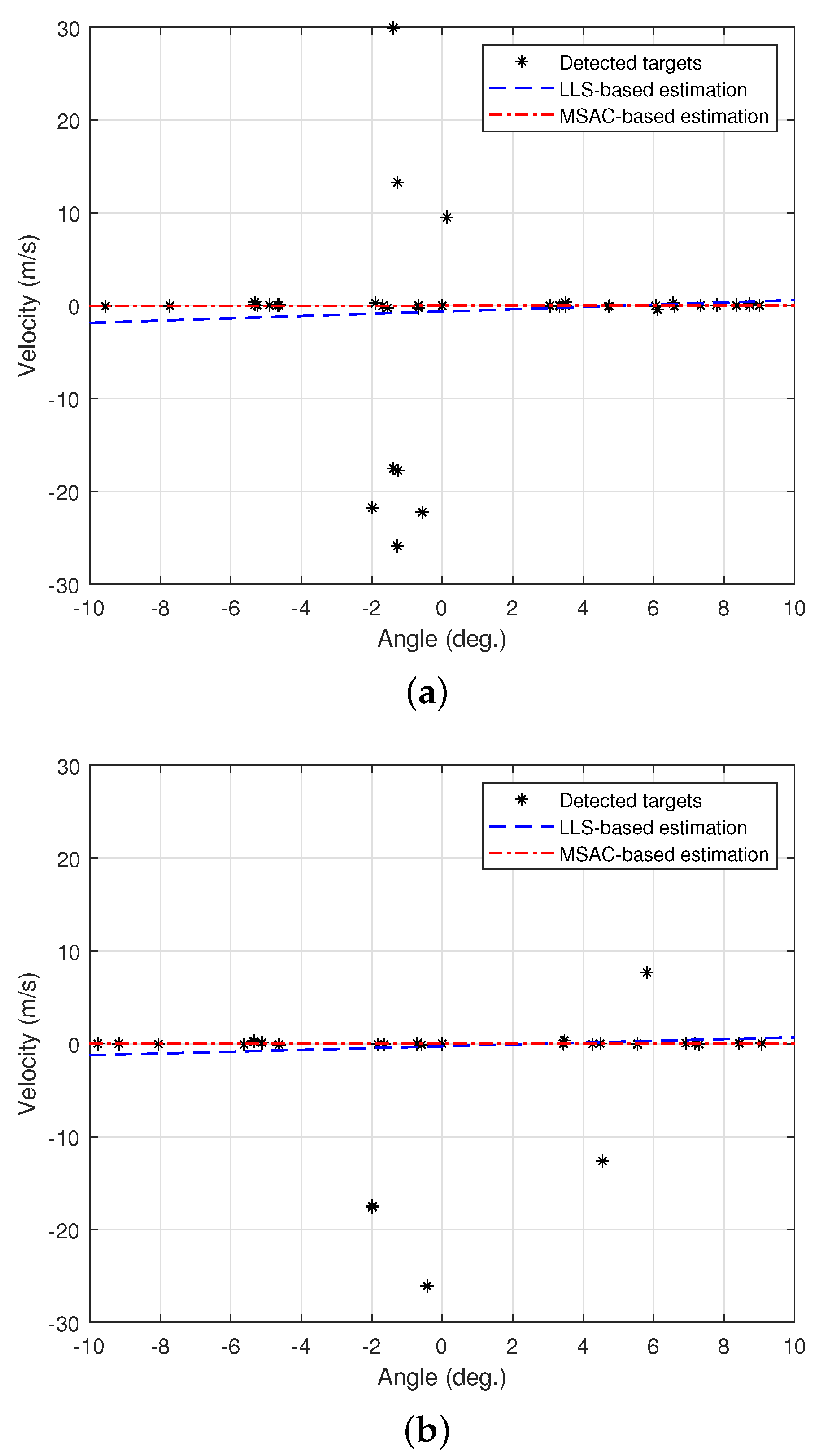
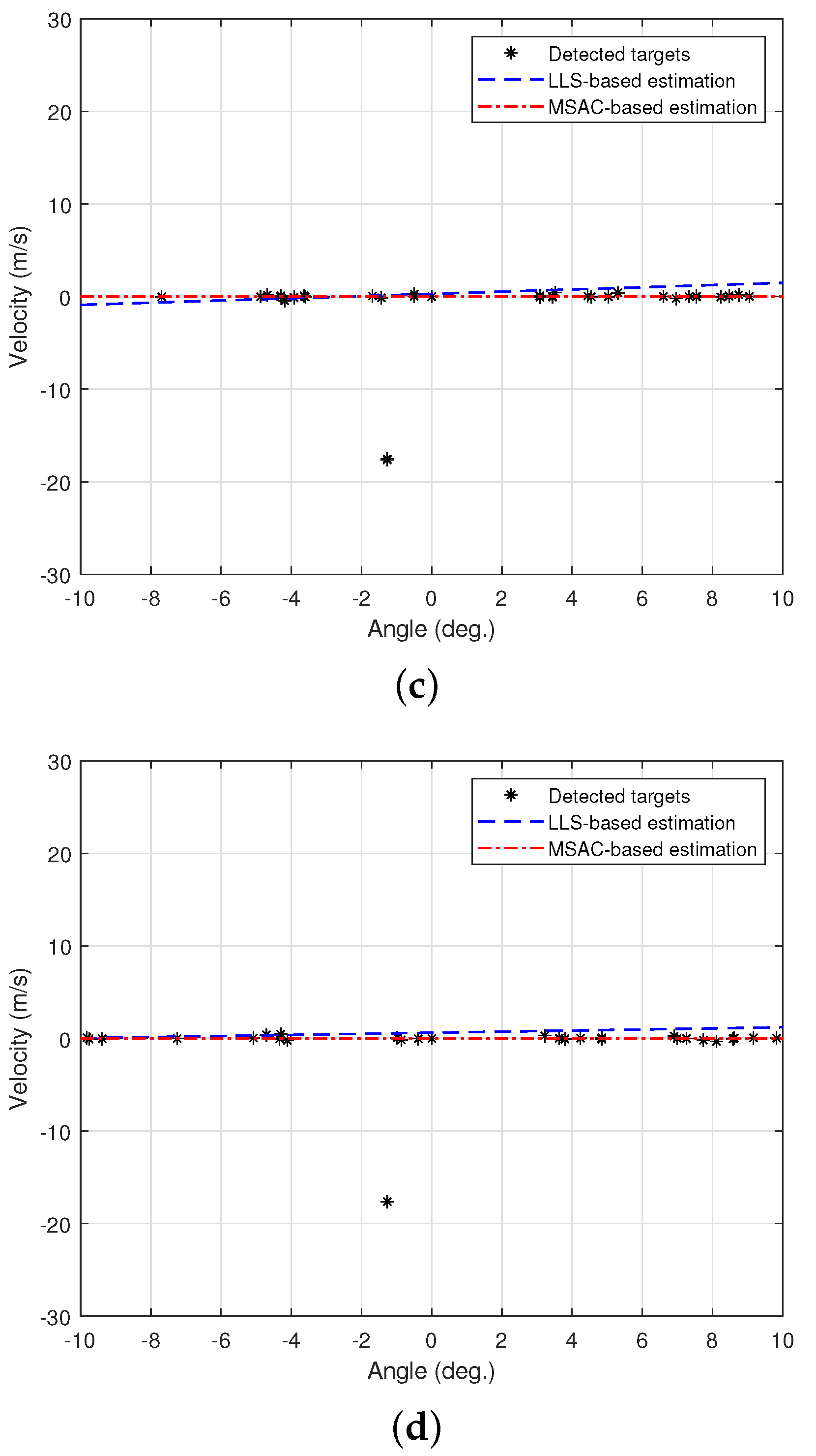
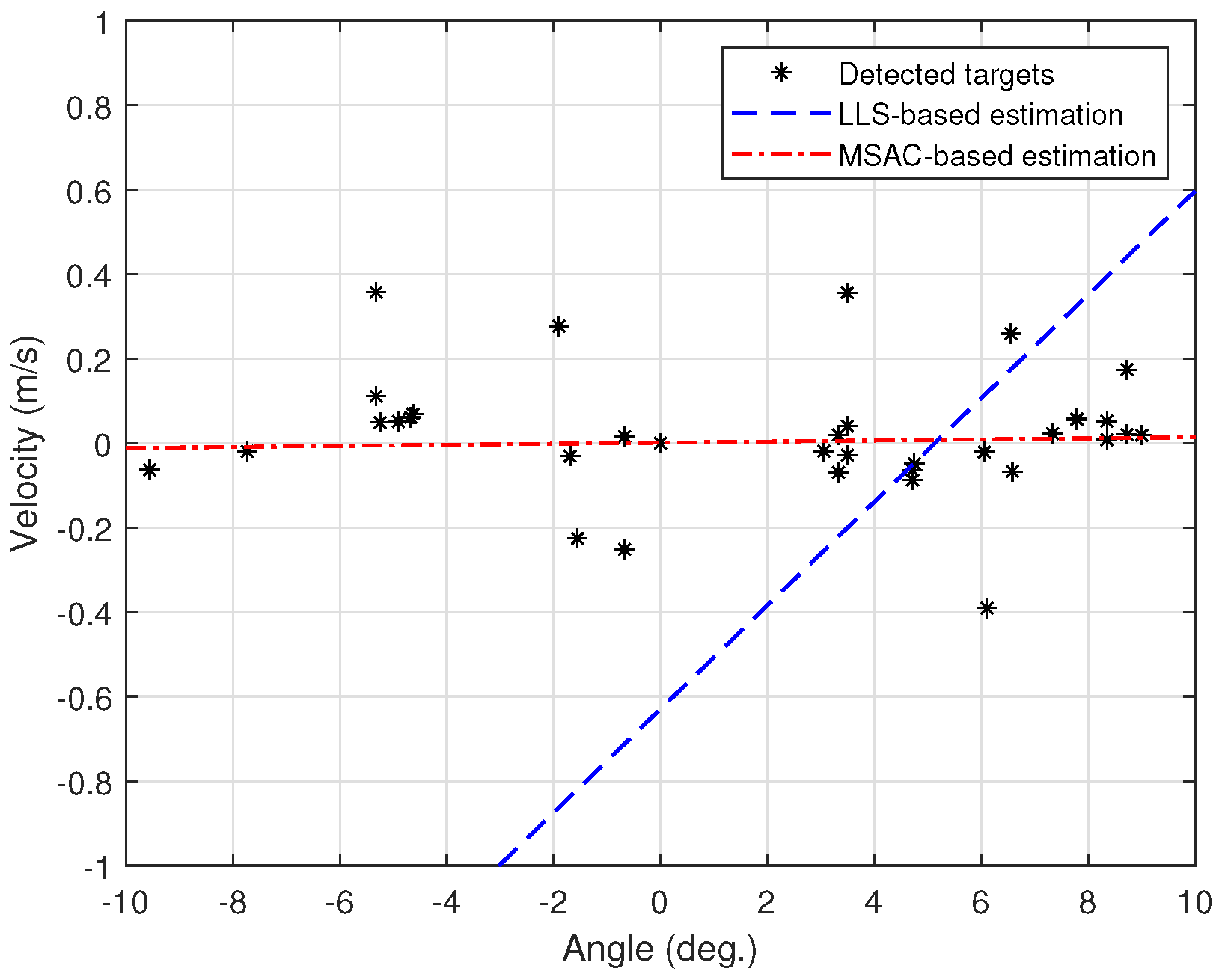
4. Proposed Stationary Target Identification Method

To classify the stationary targets in the detection results, we can simply select targets with a relative velocity of zero and remove them. However, even for a stationary target, the relative velocity cannot always be zero because the location of the target may fluctuate slightly along the radar signal reflection path. Therefore, we propose a method for discriminating stationary targets that can be applied more generally and stably. In this work, we use the detected targets in the angle-velocity domain to determine the stationary targets. Figure 8 shows the target detection results in the angle-velocity domain, which correspond to the detection results shown in Figure 7.

As shown in Figure 8a, one dominant curve can be found in the vicinity of zero velocity from the detection result. In the figure, the unit for the angle axis is degree (i.e., deg.) and the unit for the velocity axis is m/s. We can predict that stationary targets in the angle-velocity domain will exist on a specific straight line because the relative velocity is close to zero. However, as shown in Figure 8b, the velocity values of the detected points near zero velocity are not completely zero, and there is some variation around the curve.

Although general linear regression methods, such as the linear least squares (LLS) [25], are applied to the given data, an appropriate trend line cannot be found because they estimate the line using all outliers. In other words, even points corresponding to the targets with velocities greater than zero are used to find the trend line in the LLS method, which degrades the estimation performance. Thus, we use the method of RANSAC [13], which is one of the methods for fitting inliers in the presence of outliers. In the case of the RANSAC algorithm, the optimal trend line is found by iteratively estimating the line while randomly sampling the minimum points required to determine the model parameter among all the original points. Therefore, outliers are excluded from the trend line estimation, and the accuracy of the method is very high. The RANSAC algorithm is performed in the following steps:

• Several sample points are randomly selected, and model parameters are determined from the selected sample points.
• The number of sample points close to the determined model is counted.
• If the fraction of the number of inliers over the total sample points in the set exceeds a predefined threshold, re-estimate the model parameters using all the identified inliers.
• Otherwise, Steps 1 to 3 are repeated again.

In the RANSAC method, we have to set the type of function for fitting and determine how to calculate the distance between the model and the sample points. Ideally, stationary targets should be on a straight line with zero velocity, so we set the linear function for fitting. We also calculated the distance as:

$$d_i=\sum _{i=1}^M{(v_i-f\left(v_i\right))}^2,$$

(15)

where M is the total number of detected targets and $f(·)$ is the function for fitting. In addition, we set the minimum sample size and maximum distance for inliers as two and one, respectively. In our work, we used the MSAC algorithm [14], which is a enhanced version of RANSAC. The MSAC algorithm performs better than the RANSAC algorithm because the cost of the fitting function is not set uniformly for sample points, but set based on the deviation from the required functional relation [26,27].

Including the target detection results in Figure 8, we applied the proposed MSAC-based method to several successive detection results. Figure 9 shows the estimation results for the trend line.

As shown in the figure, although there are many detected points in the angle-velocity domain, the RANSAC-based estimation finds an appropriate trend line. Based on the estimated line, we can select the points with velocities close to zero. We also estimate the trend line using the LLS method. However, because the trend line is calculated using all detected points in the case of the LLS method, the accuracy decreases. For example, Figure 10 is an enlarged view of Figure 9a.

In the case of LLS-based estimation, the slope of the trend line deviates significantly from the sample points. To check the statistical performance, the slopes of the trend lines of the proposed method and the LLS method were evaluated for 100 frames, where one frame (e.g., 33 ms in Table 1) means one cycle of radar signal processing.

Table 2. Slope of the trend line.

Estimation Methods	Slope of the Trend Line
Ideal case (when the velocity is zero)	0
LLS method	0.1226
Proposed MSAC-based method	0.0013

shows the average slopes of the estimated trend lines.

Compared to the linear regression method, the proposed MSAC-based identification method estimates the slope of the trend line close to the ideal case within the algorithm parameters we set.

Finally, Figure 11 shows the reclassification result of stationary structures and moving vehicles.

In this figure, based on the classification result of the MSAC algorithm in Figure 9a, inliers and outliers are depicted in red circles and blue squares, respectively. In addition, the blue dotted line represents the boundary between the inside and outside of the road. As shown in the figure, the detection points from the moving vehicle are well classified through the proposed method. If a method of classifying stationary targets and moving targets by simply setting a threshold value for the velocity is used, it is ambiguous how to determine the threshold value. Our proposed method shows stable and reliable performance because it does not classify the points using the threshold value, but classifies them by estimating the trend in the measured data. Figure 12 shows the flowchart of our proposed signal processing technique.

5. Conclusions

In this paper, we proposed a method for discriminating stationary targets in the traffic monitoring radar system. The signal processing algorithm that automatically identifies stationary road structures is a function that must be implemented in the traffic monitoring radar system. If a stationary structure is recognized as a vehicle and this information is delivered to the driver on the road, a dangerous traffic accident can occur. We first collected raw radar data by mounting our designed FMCW radar sensor using the 24 GHz band on a road structure, such as an overpass. Then, the raw data were processed to extract various information of the targets on the road, such as the distance, velocity, angle, and radar cross-section (RCS). To classify stationary and moving targets, we used the angle-velocity domain characteristics of the targets. Unlike in the two-dimensional x-y range map, stationary targets existed around the straight line with zero velocity in the angle-velocity domain. Thus, in this domain, there is the advantage that moving targets and stationary targets are clearly distinguished. Finally, to find the inliers on the straight line, we used the MSAC algorithm and verified its performance using the actual radar measurement results. As a result of checking the slopes of the estimated trend lines in successive frames, the estimation accuracy of the proposed method was higher compared to the LLS-based method because it does not estimate the trend line using all detected points. In addition, the proposed identification method has an advantage in that it can be applied in real time due to its small amount of calculation. We believe that the proposed method is essential for stable detection performance in traffic monitoring radar systems. Including discriminating stationary targets, we plan to conduct research on how to classify the types of moving vehicles, such as sedans, sports utility vehicles, or trailers.

References

1. Cheng, H.-Y. Camera placement based on vehicle traffic for better city security surveillance. IEEE Intell. Syst. 2018, 33, 49–61. [Google Scholar]
2. Ma, X.; He, Y.; Luo, X.; Li, J.; Zhao, M.; An, B.; Guan, X. Highway traffic flow estimation for surveillance scenes damaged by rain. IEEE Intell. Syst. 2018, 33, 64–77. [Google Scholar]
3. Ho, G.T.S.; Tsang, Y.P.; Wu, C.H.; Wong, W.H.; Choy, K.L. A computer vision-based roadside occupation surveillance system for intelligent transport in smart cities. Sensors 2019, 19, 1796. [Google Scholar] [CrossRef] [PubMed] [Green Version]
4. Samczynski, P.; Kulpa, K.; Malanowski, M.; Krysik, P.; Maślikowski, Ł. A concept of GSM-based passive radar for vehicle traffic monitoring. In Proceedings of the Microwaves, Radar and Remote Sensing Symposium, Kiev, Ukraine, 25–27 August 2011. [Google Scholar]
5. Krysik, P.; Kulpa, K.; Baczyk, M.; Maślikowski, Ł.; Samczynski, P. Ground moving vehicles velocity monitoring using a GSM based passive bistatic radar. In Proceedings of the 2011 IEEE CIE International Conference on Radar, Chengdu, China, 24–27 October 2011. [Google Scholar]
6. Felguera-Martín, D.; González-Partida, J.-T.; Almorox-González, P.; Burgos-García, M. Vehicular traffic surveillance and road lane detection using radar interferometry. IEEE Trans. Veh. Technol. 2012, 61, 959–970. [Google Scholar] [CrossRef] [Green Version]
7. Gómez-del-Hoyo, P.; Bárcena-Humanes, J.L.; Mata-Moya, D.; Juara-Casero, D.; Jiménez-de-Lucas, V. Passive radars as low environmental impact solutions for smart cities traffic monitoring. In Proceedings of the International Conference on Computer as a Tool (EUROCON), Salamanca, Spain, 8–11 September 2015. [Google Scholar]
8. Cao, L.; Wang, T.; Wang, D.; Du, K.; Liu, Y.; Fu, C. Lane determination of vehicles based on a novel clustering algorithm for intelligent traffic monitoring. IEEE Access 2020, 8, 3892–3901. [Google Scholar] [CrossRef]
9. Lee, H.-B.; Lee, J.-E.; Lim, H.-S.; Jeong, S.-H.; Kim, S.-C. Clutter suppression method of iron tunnel using cepstral analysis for automotive radars. IEICE Trans. Commun. 2017, E100-B, 400–406. [Google Scholar] [CrossRef]
10. Yoon, J.; Lee, S.; Lim, S.; Kim, S.-C. High-density clutter recognition and suppression for automotive radar systems. IEEE Access 2019, 7, 58368–58380. [Google Scholar] [CrossRef]
11. Lee, S.; Yoon, Y.-J.; Yoon, J.; Sim, H.; Kim, S.-C. Periodic clutter suppression in iron road structures for automotive radar systems. IET Radar Sonar Navig. 2018, 12, 1146–1153. [Google Scholar] [CrossRef]
12. Song, H.; Shin, H.-C. Classification and spectral mapping of stationary and moving objects in road environments using FMCW radar. IEEE Access 2020, 8, 22955–22963. [Google Scholar] [CrossRef]
13. Torr, P.H.S.; Zisserman, A. MLESAC: A new robust estimator with application to estimating image geometry. Comput. Vis. Image Underst. 2000, 78, 138–156. [Google Scholar] [CrossRef] [Green Version]
14. Fischler, M.A.; Bolles, R.C. Random sample consensus: A paradigm for model fitting with applications to image analysis and automated cartography. Commun. ACM 1981, 24, 381–395. [Google Scholar] [CrossRef]
15. Hartley, R.; Zisserman, A. Multiple View Geometry in Computer Vision; Cambridge University Press: Cambridge, UK, 2004. [Google Scholar]
16. Bitsensing Inc., ATM210. Available online: http://bitsensing.com/pdf/200526/Technical_Specification_AIR_Traffic_Radar_1.0.pdf (accessed on 25 June 2020).
17. Rohling, H.; Meinecke, M.-M. Waveform design principles for automotive radar systems. In Proceedings of the CIE International Conference on Radar Proceedings, Beijing, China, 15–18 October 2001. [Google Scholar]
18. Winkler, V. Range Doppler detection for automotive FMCW radars. In Proceedings of the European Radar Conference, Munich, Germany, 9–12 October 2007. [Google Scholar]
19. Krim, H.; Viberg, M. Two decades of array signal processing research: The parametric approach. IEEE Signal Process. Mag. 1996, 13, 67–94. [Google Scholar] [CrossRef]
20. Patole, S.M.; Torla, M.; Wang, D.; Ali, M. Automotive radars: A review of signal processing techniques. IEEE Signal Process. Mag. 2017, 34, 22–35. [Google Scholar] [CrossRef]
21. Gross, F. Smart Antennas for Wireless Communications; McGraw-Hill: New York, NY, USA, 2005. [Google Scholar]
22. Schmidt, R. Multiple emitter location and signal parameter estimation. IEEE Trans. Antennas Propag. 1986, 34, 276–280. [Google Scholar] [CrossRef] [Green Version]
23. Lee, S.; Yoon, Y.-J.; Kang, S.; Lee, J.-E.; Kim, S.-C. Enhanced performance of MUSIC algorithm using spatial interpolation in automotive FMCW radar systems. IEICE Trans. Commun. 2018, E101-B, 163–175. [Google Scholar] [CrossRef]
24. Kang, S.; Lee, S.; Lee, J.-E.; Kim, S.-C. Improving the performance of DOA estimation using virtual antenna in automotive radar. IEICE Trans. Commun. 2017, E100-B, 771–778. [Google Scholar] [CrossRef]
25. Boyd, S.; Vandenberghe, L. Convex Optimization; Cambridge University Press: Cambridge, UK, 2004. [Google Scholar]
26. Chen, H.; Meer, P. Robust regression with projection based M-estimators. In Proceedings of the Ninth IEEE International Conference on Computer Vision, Nice, France, 13–16 October 2003. [Google Scholar]
27. Choi, S.; Kim, T.; Yu, W. Performance evaluation of RANSAC family. In Proceedings of the British Machine Vision Conference, London, UK, 7–10 September 2009. [Google Scholar]
Figure 1. Traffic monitoring radar installed on the overpass.
Applsci 10 05838 g001
Figure 2. Traffic monitoring radar developed by Bitsensing Inc.
Applsci 10 05838 g002
Figure 3. Antenna system of our traffic monitoring radar: one transmit antenna element and four receiving antenna elements.
Applsci 10 05838 g003
Figure 4. Schematic block diagram for radar signal processing.
Applsci 10 05838 g004
Figure 5. Frequency change of the waveform over time.
Applsci 10 05838 g005
Figure 6. Method of estimating the position of the target using the radar detection result.
Applsci 10 05838 g006
Figure 7. Target detection result in the Cartesian coordinate system.
Applsci 10 05838 g007
Figure 8. Target detection results in the angle-velocity domain: (a) velocity ranges from −40 m/s to 40 m/s (b) velocity ranges from −1 m/s to 1 m/s (same data as Figure 8a, but reduced velocity range).
Applsci 10 05838 g008
Figure 9. Estimation results for successive detection results: (a) t = 0 (ms); (b) t = 33 (ms); (c) t = 66 (ms); (d) t = 99 (ms).
Applsci 10 05838 g009aApplsci 10 05838 g009b
Figure 10. Estimation result: velocity ranges from −1 m/s to 1 m/s (same data as Figure 9a, but reduced velocity range).
Applsci 10 05838 g010
Figure 11. Reclassification result for detected targets.
Applsci 10 05838 g011
Figure 12. Flowchart of the proposed method (inside the DSP).
Applsci 10 05838 g012