1. Introduction
Intelligent traffic monitoring is an important technology component of modern smart cities and traffic monitoring systems. One of its components is traffic analysis from closed-circuit television (CCTV) cameras that are placed at the roadside. Applications, such as vehicle counting/classification and speed measurement, provide important statistics that can be used to improve traffic flow. A recent smart city challenge organised by NVIDIA [
1] confirms the significance of these problems. Such solutions can bring many benefits to transportation systems. However, several requirements need to be satisfied:
the system needs to work in a fully automatic mode. Hence no extra manual supervision or annotations should be necessary so that the workload required when deploying the system is minimised; and,
real-time performance with power-efficient computing is required, as it might be desirable to deploy the system on an embedded platform.
A crucial component of such a system is vehicle detection (optionally also including their categorisation), which provides a means for accurate vehicle tracking. Recently, most of the object detection benchmarks have been dominated by methods that are based on Convolutional Neural Networks (CNNs). One of the reasons behind this success is the availability of large-scale annotated datasets, i.e., UA-Detrac [
2] and Kitti [
3]. However, the problem is still far from being considered as solved. The above methods may bring impressive results when they are tested under conditions similar to those in which the training set was captured; however, CNN-based approaches are known to be extremely vulnerable to small changes in the distribution of the images: adding a small amount of Gaussian noise [
4,
5] or small translations/rotations of the input image [
6] or changes in the lighting [
7] may drastically change the output of the model. This problem could be solved by collecting extra annotations from the deployment environment and by including that data in the neural network training, but such a scenario is not always possible. When considering a traffic monitoring system that is to be deployed to many places around the city with different camera views, it is evident that it would be very difficult to collect a large and representative annotated dataset.
Most of the approaches to vehicle monitoring systems assume that, once the system is deployed, it is not updated anymore [
8,
9]. While that approach simplifies the deployment, maintainability, and reduces the cost of the system, there is room for improvement. As a camera observes moving vehicles in a static scene, several cues can be obtained. Firstly, a reliable model of the background should be created in order to identify some of the false positive detections. Secondly, the tracking system may further improve open detections by taking into account temporal cues. All of this information can be used to generate reliable labels from the video stream withot human supervision and to further fine-tune the model based on those labels. Such an approach is known as semi-supervised learning (SSL) where an initial annotated training dataset is available, as well as a stream of unlabelled data. Meanwhile, a major challenge in any SSL technique is semantic drift, i.e., if some of the new samples are wrong, they may cause the model to drift away from the original concept.
Semi-supervised learning applied to video analysis from a stationary camera is an approach that can potentially enable a reduction of the number of noisy labels to a minimum. In recent work, it was shown that, by careful design and by taking many cues into account, such as appearance, motion, and temporal coherency, it is possible to significantly improve the accuracy of the initial detector [
10]. In this work, a similar approach is followed, and, by means of tracking and background modelling reliable pseudo-labels, are obtained, which are further used for fine-tuning of the model. To achieve real-time processing on an embedded platform, an energy-efficient CNN, called SqueezeDet, is employed [
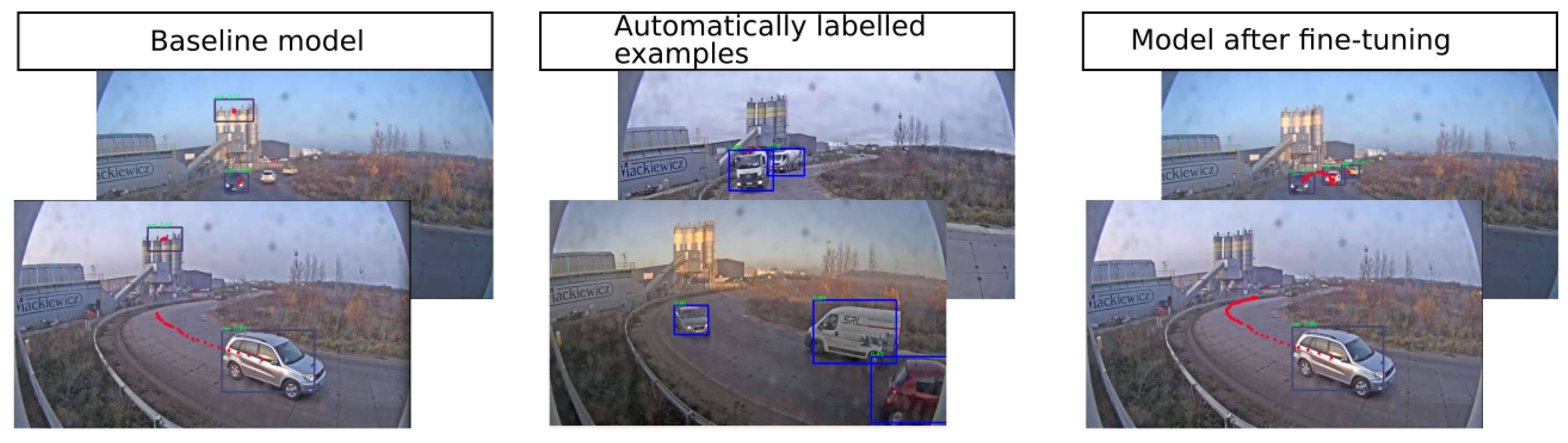
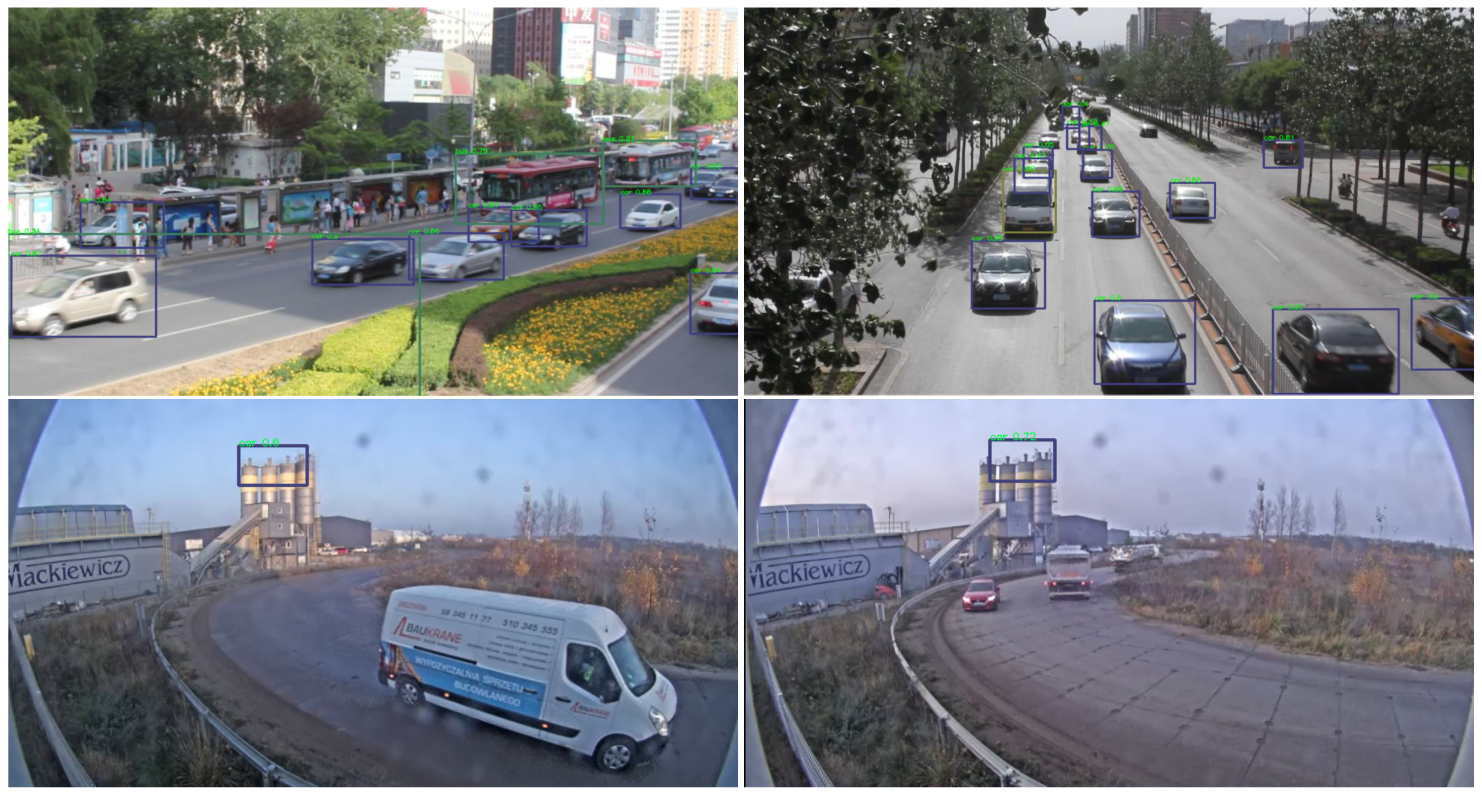
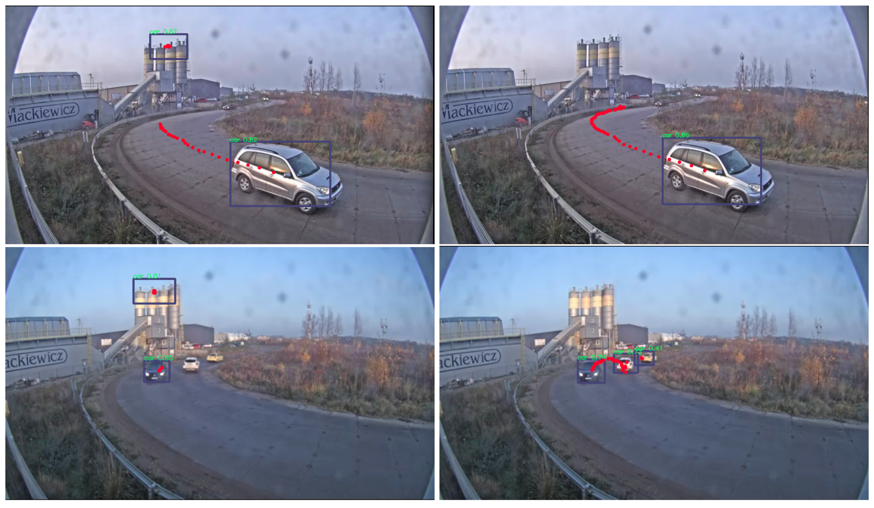
11]. Our idea is illustrated in
Figure 1, where models trained on a dataset perform well in the case that the test data are similar to the training set. However, when deployed to a new environment, those models may fail in seemingly simpler cases (see the left column). Therefore, automatically collected labels are applied for fine-tuning the baseline model (as in the center column). After fine-tuning of the model, the vehicles are more successfully tracked for a bigger number of frames and some vehicles located at the far end are more efficiently recognised (
Figure 1—right column).
To summarise, in this work, the focus is on developing a system for traffic monitoring. Firstly, the proposed system is deployed to the embedded Jetson Tx2 platform. Further, adaptation methods are employed in order to improve the efficiency of the deployed system in a real-world scenario. With the ubiquitous presence of such cameras in cities around the world, there is great potential for practical implementations of solutions of this kind. Finally it is assumed that no labelled data from the target environment is available, which is a realistic scenario. The contribution of this paper is, as follows:
the SqueezeDet algorithm is adjusted for vehicle detection on an embedded platform, and the accuracy on UA-Detrac dataset and its performance on a Jetson TX2 under different input image resolutions is reported,
automatic labelling is applied for one of our cameras. Data are collected for several days, and fine-tuning happens at the end of each day. This procedure results in a substantial increase in vehicle detection accuracy, as explained in the section devoted to the discussion of the results, and
experiments on the human-in-the-loop scenario are performed, which further increases the efficiency of the detection.
2. Related Work
Vehicle detection. Historically, background subtraction algorithms were often used for vehicle tracking [
12,
13]. These methods work well in good weather conditions, and with a moderate traffic density. However, they fail in various illumination conditions (shadows, car lights in use at night), and in the case of high-density traffic. However, despite these disadvantages, these kinds of methods are commonly used, because they can often be deployed directly with no training nor calibration required.
Vehicle detection falls into the category of object detection methods, which have recently been dominated by CNN-based methods. Recent comparative works on vehicle detection confirm this advantage [
9,
14,
15]. One of the first algorithms that yielded impressive results was R-CNN [
16]. For each image, around 2000 object-agnostic region proposals were computed while using Selective Search [
17], and for each image, obtained CNN features were classified by support-vector-machine (SVM). Such a model for each region proposal (bounding box) returns a vector of class probabilities to which the given box belongs. Unfortunately, the performance was very low, with region definitions being the main bottleneck. Later region proposals were integrated into CNNs in an end-to-end manner in Faster-RCNN [
18]. The demand for faster inference resulted in so-called one-stage detector networks, such as YOLO [
19], SSD [
20], and SqueezeDet [
11]. Those models directly predict bounding box locations and class probabilities with a single network in a single attempt. The image is divided into
W * H cells, and each cell is directly responsible for detecting objects. As a result, a much faster inference is achieved with a small loss in accuracy.
It is only recently that deep learning has started to be used by intelligent transportation systems. Out of all of these algorithms, currently, only one-stage detectors are capable of obtaining real-time performance with limited computing power. However, most of the recent work in vehicle detection has focused on obtaining the best accuracy by using models utilising specialised GPUs [
21,
22]. Therefore, one of the objectives of this work is to estimate what accuracy can be achieved on embedded systems, i.e., NVIDIA Jetson Tx2. That is why the efficient SqueezeDet architecture was used for vehicle detection. Details of that algorithm are recalled in the next section.
Vehicle tracking. Object tracking methods can be divided, in general, into online and offline methods. In the online case, only the current frame is available for the processing, while in offline methods, a sequence of frames is considered at once [
23]. Having precomputed detections along the whole video sequence, different optimisation algorithms can be used for finding object trajectories, e.g., by energy minimisation [
24]. However, in this work, we are interested, in on-line object tracking, as it is intended to be applied directly to practical traffic monitoring systems. Held et al. [
25] used a CNN that was trained to regress directly from two images the location in the second image of the tracked object shown in the first image. Another recent work uses Siamese Networks for object tracking [
26]. One of the advantages of such methods is that they can track an arbitrary object as long as the initial bounding box is given for that object. However, those works focus on single-object-tracking, and they require an initial bounding box that is not available in the real-world scenario of traffic monitoring.
When compared to single-target-based, multi-object-tracking (MOT) is much more complicated due to the varying number of objects, and the interactions between these objects. Tracking-by-detection is a dominating paradigm in MOT. The algorithm is composed of three steps: detection, prediction, and association. First, the object detector is run on a target image. The prediction model is used for estimating all objects’ new positions given their current states. Finally, the association model is applied for associating the currently tracked objects with new detections. In recent work, vehicle motion is modelled with group behaviour [
27]. In the approach, named SORT [
28], Kalman filtering is used for the prediction step, and the Hungarian algorithm is implemented for the association between the existing tracked vehicles and new detections. It is a very efficient and accurate method with the only drawback being the lack of handling long-term occlusions. This was later fixed by utilising recent advances in Deep Learning to learn the association metric [
29]. Unfortunately, this approach requires training and also more computation power engagement. Another approach uses computing Wasserstein distance as association metric allowing for obtaining very good vehicle tracking performance, however is also computationally expensive [
30]. In more recent work, Bochinski et al. used a very straightforward method working without any prediction model [
31]. It works on the assumption that dense frames are available for tracking. In the real world, this assumption does not always hold, especially when performing tracking on embedded systems, where only a few frames per second are available. This is why, in this work, the SORT tracker was used.
Domain Adaptation. Appearance changes based on lighting, weather conditions, and also because different class distributions of objects provide a significant challenge for systems relying on machine learning models for perception. Trained models are biased towards the datasets they were trained on, and the model performance drops in the test domain when the conditions are different. In particular, it is impossible in many situations to collect and annotate a representative dataset. To overcome this issue, many methods that fall into the category of domain adaptation have been proposed. Sometimes it is assumed that a limited amount of annotated data is available in the target domain [
32], however such a scenario is not always feasible, which is why we focus on unsupervised adaptation. One of the approaches assumes learning a transformation that maps feature representations from the target domain to the source domain [
33].
A popular technique is a self-training method, which involves creating an initial baseline model on fully labelled data, and then exploiting this model to estimate labels on a novel unlabelled dataset. The obtained pseudo-labels are further used for model fine-tuning. Such a method was successful, for example, in the semantic segmentation domain [
34,
35]. One of the challenges in this technique is the fact that pseudo-labels can be inaccurate. However, because a video stream is analysed, the temporal coherency, and motion modelling can provide additional cues that can improve adaptation. One of the first approaches was revealed in the work of Koller et al. [
36], where labels were automatically found in the target domain using object tracking, and they were later used for model fine-tuning. Recent work models the data in multiple feature spaces to further reduce the number of false positives using the decorrelated error technique [
10]. We are inspired by these works, and employ tracking and background modelling to assure efficiency in automatically obtained labels.
The fine-tuning of the model on automatically labelled data only might result in catastrophic forgetting of previously learned information [
37]. The rehearsal technique, in which, during the fine-tuning, automatically labelled data are mixed with the data that the model was initially trained with, has proven to be effective in minimising such an effect [
38]; hence, this technique is used in our work. Moreover, adding a minimal amount of human effort might be beneficial for the machine learning system [
39]. Consequently, experiments with such a human-in-the-loop scenario were performed, and inaccurate automatically obtained labels were manually filtered out.
3. Methods
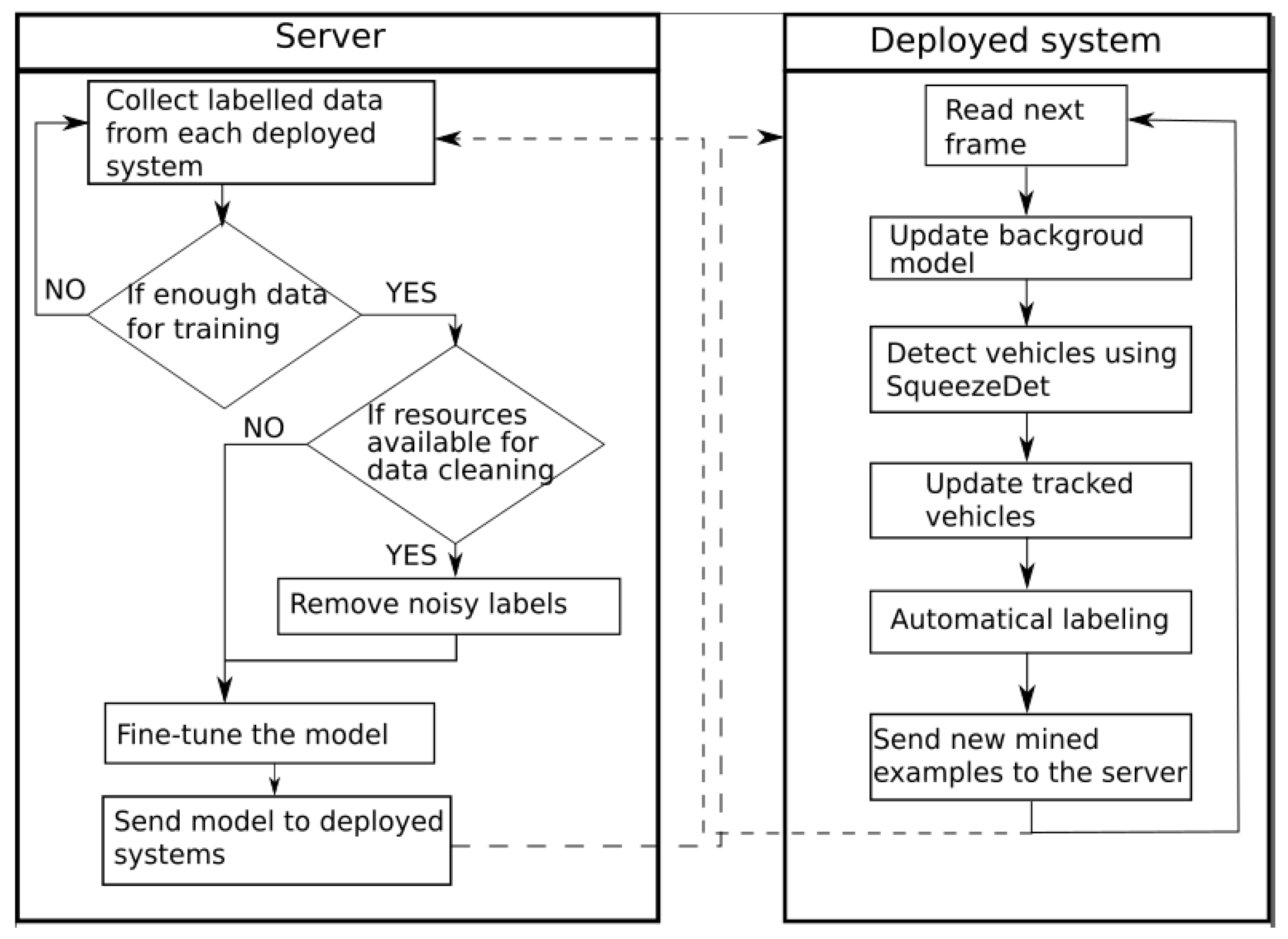
In this section, our method for automatic adaptation of the deployed detector is presented (
Figure 2). The deployed system consists of a camera and an embedded platform that is responsible for real-time traffic analysis, and for sending all relevant information to the main server. The core server collects the data from all endpoints, and fine-tunes the models, which are sent back to the deployed systems, meaning that all of the systems share the same detection model. Finally, if possible, a human might filter the automatically obtained samples by simply removing samples with wrong annotations. That allows us to further improve the efficiency of the model with minimal human effort required. The SqueezeDet architecture that was used for detection is described in
Section 3.1, the SORT tracking method in
Section 3.2, and the introduced labelling module with fine-tuning details in
Section 3.3.
3.1. Vehicle Detection
In this work, SqueezeDet was applied for vehicle detection. In this section, the main components of the architecture and loss function are briefly described. SqueezeDet is a lightweight, single-shot, fully convolutional object detection architecture developed recently for applications in autonomous vehicles. The design objectives (efficiency and accuracy) make it perfect for the traffic monitoring system on an embedded platform.
As SqueezeDet processes an image, the first step is the extraction of a high dimensional, low-resolution feature map (as in other CNN architectures). Having obtained feature map representation, the goal is to predict the bounding boxes of the vehicles in the input image. SqueezeDet falls into the category of one-stage detectors. A W * H grid is defined over an image, where W and H are the number of grid cells along the horizontal and vertical axes. At each element of the grid, there are K bounding boxes with predefined size, which are called anchor boxes. Each anchor is defined by four scalars: , , , , where i [1,W], j [1,H] and k [1,K]. , , stand for spatial coordinates of (i, j) grid center, and , are the width and height of k-th bounding box. The anchors define the a priori distribution of the size of bounding-boxes. In total, there are W * H * K anchors that are responsible for detecting objects.
One-stage detectors further learn how to refine the initial window to match the true location of the object. Hence, for each
i,j,k-anchor four relative coordinates
,
,
,
are computed that transform the anchor into final bounding box prediction [
11]:
where
,
,
, and
are the final coordinates predictions of the detected object. Each anchor also returns
C + 1 values where the first value is a confidence score which determines how likely it is that the given bounding box contains an object. The other
C scalars represent the conditional probability distribution for each of
C predefined classes.
Consequently, SqueezeDet returns W * H * K predictions in total. Then, as a post-processing step, the top N predictions with the highest confidence score are used for further processing with the Non-Maximum Suppression (NMS) algorithm, which removes the redundant boxes. This is a procedure that looks for pairs of boxes for which the intersection-over-union (IOU) is bigger than a selected threshold, and it removes boxes with a lower confidence score.
During training, the SqueezeDet is supervised with training samples where, for each image, a list of ground truth bounding boxes (x, y, w, h), and its corresponding class c, is given. The objective of the training phase is to update the weights of the neural network, so that the output from the detector matches the ground truth as closely as possible. This is achieved by defining a loss function that is optimised through backpropagation.
The loss function is defined, as follows [
11]:
where (
,
,
,
) are the ground truth bounding boxes. The first part of the loss function is the bounding box regression that assures that
ijk-anchor, which is the closest to the ground truth box returns
,
,
,
parameters that will fit ground truth bounding box parameters. During the training the ground truth boxes are compared with all anchors and assigned to the anchor box with the highest overlap (IOU) with ground truth. This means that only the closest anchor is accountable for detecting a given object. This operation is achieved by
which evaluates to 1 if
ijk-anchor has the highest IOU with the ground truth box, 0 otherwise. Finally, because there might be multiple objects in the image, the value is divided by the number of objects
.
The second part in the loss function is the confidence score regression. The goal here is twofold: assure that the closest anchor confidently detects an object, and to penalise the other anchors for false positive detections. is the confidence score from ijk-anchor of how likely it contains an object. is the IOU between accountable ijk-anchor and the ground truth. At the same time, the confidence scores of all other boxes are penalised with where and normalised by the number of anchors (WHK) minus the number of objects in the image.
The last part of the loss function is a cross-entropy loss for the classification of the object. The loss function defines three hyperparameters:
,
, and
, which adjust the weights of the loss components. In our training, the same values were used as in the original paper [
11],
= 5,
= 75,
= 100. The loss function is optimized directly through back-propagation, which updates the weights of the neural network.
3.2. Vehicle Tracking
In this work, the SORT approach is applied for vehicle tracking [
28]. This method follows the tracking-by-detection framework. Firstly, the object detector returns bounding box proposals for a given frame. In the next step, new detections are associated with existing ones (called tracks) by using the Hungarian algorithm [
40]. The vehicle motion is estimated using the Kalman filter to improve the tracker accuracy further [
41]. This framework provides great efficiency with very good accuracy in an online setting.
The goal of the vehicle association step is to match the new bounding box detections returned by the vehicle detector with the existing tracks. Firstly the IOU between all new detections and all existing tracks is computed. This forms a cost matrix, and the problem is to find an association where the cost is minimal. Cost is defined as a sum of all unassigned values in the cost matrix. There are many methods for solving this problem, e.g., sub-optimal, but a fast greedy algorithm that first assigns the biggest values to the cost matrix. However, the optimal solution can be found using the Hungarian algorithm. Additionally, a minimum constraint is added to remove possible false assignments with a small overlap. All of the detections that were not matched form new tracks.
Next, the vehicle’s motion needs to be modelled. Given the history of the vehicle’s positions, its location in a subsequent frame can be approximated. Additionally, because the observation model (vehicle detector) is not perfect (detections may be inaccurate or missing), a tracking method is needed that accounts for this uncertainty in the model. For this purpose, the Kalman filter is applied. Each vehicle is modelled as a vector [
28]:
where
u and
v are horizontal and vertical pixel positions of vehicle bounding box centroid,
s stands for scale (area) and
r for the ratio of the bounding box.
u, v, s, r are the measurements, while
,
, and
are estimated from observations. To track a moving vehicle, two basic procedures are applied:
A new detection that was not matched to any of the existing tracks creates a new identity with a unique identifier initialised with zero velocity and geometry of the bounding box. Because this is a first detection of the vehicle, and its velocity is not known, large values of the velocity component in covariance matrix P are assigned, reflecting uncertainty regarding the speed. Tracks are removed if they are not detected for frames. This solution allows for handling short-term occlusions, and it resolves situations where the detector fails to detect an existing vehicle for a few frames. However, the valuue of should be kept relatively small to prevent uncontrolled growth in the number of tracks.
Finally, it is possible to add a probationary period, during which the vehicle is regarding as not being active, i.e., a track is considered to be active when it has successfully been tracked for consecutive frames. This helps to prevent the tracking of some false positively detected objects. In our experiments, the values of the covariance matrices were initialised with the same values as in the original SORT paper, and the following values were used— = 0.5, = 2, and = 2.
3.3. Automatic Labelling and Fine-Tuning
The goal of this stage is to collect a set of training images with corresponding labels that will be used later for automatic fine-tuning of the network with the expected effect of improvement of the detection accuracy of the model in the deployed environment. However, there is no point in collecting superfluous samples, namely those for which the neural network is already confident enough. Intuitively, the use of similar samples for fine-tuning would not bring many benefits to the accuracy of the classifier. Additionally, a considerable number of the detection results returned by the neural network are inaccurate. Consequently, the main challenge here is keeping the number of noisy labels as low as possible.
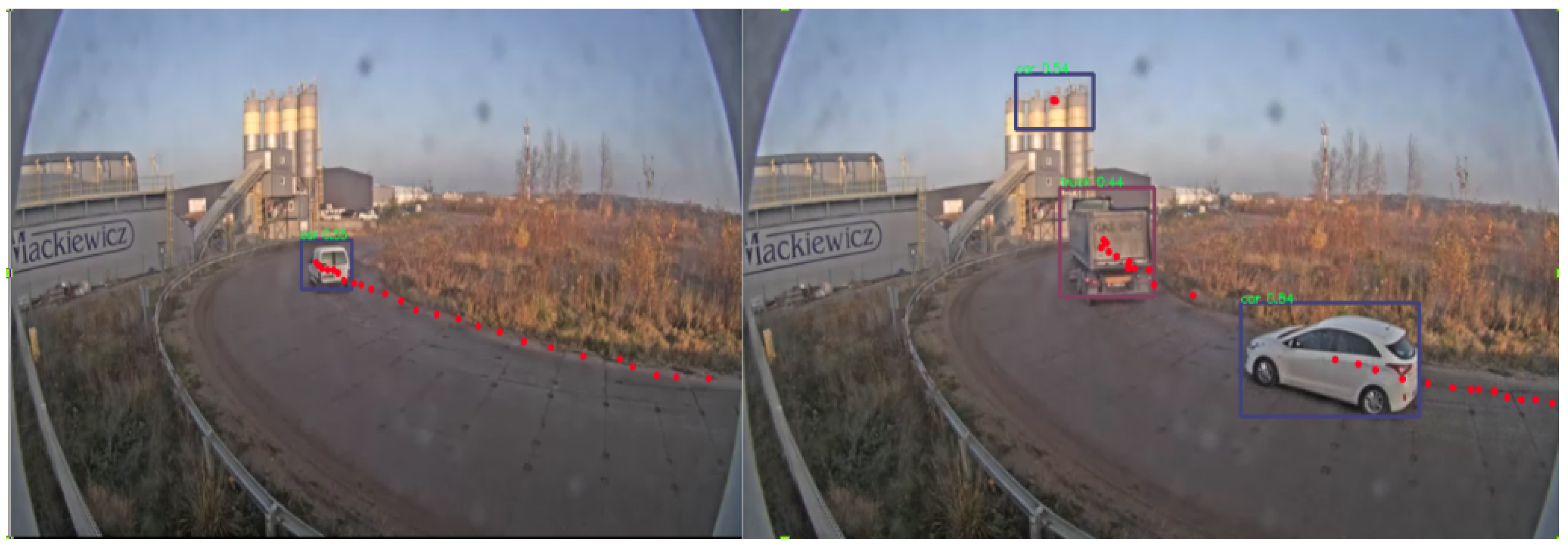
Our algorithm for obtaining labels automatically is based on two observations (
Figure 3):
some of the vehicles are tracked for dozens of frames, but still, the confidence of the object detector is very low. Long, high confidence tracks can be collected, and from those, it is possible to find vehicle detections predicted with low confidence. Those samples can be used then for the fine-tuning of the neural network, which should increase the accuracy of the classifier; and,
some background static objects are detected as vehicles. Those objects can be filtered out using a background model.
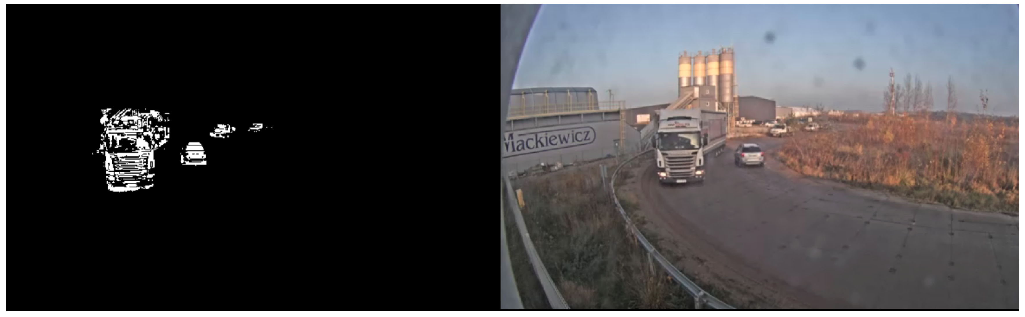
Because the traffic monitoring system works with a static camera, a reliable model of the background can be created to improve the detector accuracy. For this purpose, a popular background subtraction method created by Bowden et al. [
42] is used. It is a Gaussian Mixture-based method, where each pixel is modelled by a mixture of K Gaussian distributions (K = 5 is used in our experiments).
Figure 4 shows an example of the foreground/background separation.
Pseudo-code of our algorithm for automatic labelling is presented in the Algorithm 1. First, tracks with high confidence are saved, i.e., those that were tracked for at least
consecutive frames or at least one of the detections had high confidence (lines 4–5). Such a definition can still entail some noisy labels; hence, the background subtraction algorithm to differentiate between the background and moving objects in the scene is used. From the detected objects, those that contain no more than
* 100% moving pixels are filtered-out (line 20). Because a one-stage detector is used in our work, it means that the whole scene is used for the training of our detector, which may still fail to detect some of the objects in the scene. To minimise the number of such examples, the background model is used again. Specifically, a candidate frame is accepted if at least
* 100 % of the foreground pixels are exploited with regard to detections (line 30). In our experiments, the following constants were used
,
,
,
,
, and
.
| Algorithm 1 Extract Labels |
| Input: image, tracks, fg_mask | ▹ fg_mask = foreground mask |
| Output: detections | ▹ return filtered detections |
| |
| 1: |
| 2: |
| 3: for all trk in tracks do | ▹ For all trackers |
| 4: if trk.conf in range (, ) then | ▹ If low- confidence detection |
| 5: if trk.length or trk.maxConf > then | ▹ confident tracker |
| 6: |
| 7: |
| 8: if and then |
| 9: return tracks.bboxes | ▹ return filtered bounding boxes |
| 10: else return None |
| 11: |
| 12: procedure FilterTracks(tracks, fg_mask) | ▹ Filter out tracks that belong to the background |
| 13: |
| 14: for all trk in tracks do |
| 15: |
| 16: |
| 17: |
| 18: |
| 19: if then | ▹ If at least % pixels are foreground |
| 20: |
| 21: return |
| 22: |
| 23: procedure IsMotionCovered(tracks, fg_mask) ▹ Return true if foreground objects are detected |
| 24: | ▹ number of fg pixels |
| 25: for all trk in trackers do | ▹ For all trackers |
| 26: 3 |
| 27: | ▹ not covered pixels |
| 28: |
| 29: return |
The model gets fine-tuned after the automatically labelled samples are collected. To prevent catastrophic forgetting, a popular rehearsal technique is used, where the initial data (on which the model was trained) is mixed with new data during the fine-tuning stage [
38]. One of the drawbacks of this method is that it requires access to a lot of data storage. However, because in our architecture, the model is fine-tuned on the core server, there are no strict storage constraints in this case.
Our labelling procedure works on the assumption that it is possible to train an initial model that will perform sufficiently in the deployment environment so that it can obtain confident tracks of at least some objects. This assumption is met for objects for which a large database is available, i.e., for vehicles. However, the main drawback of the presented method is the use of the one-stage detector in which a whole frame is being employed for neural network training. This means that all of the objects in the scene should be correctly annotated in this case. This stands in contrast to the exemplar-based method [
24], where sparse labels (a bounding box only around the single object of interest) are used. Yet, because the goal is real-time performance on embedded systems, and utilising advances in CNNs, the one-stage detector is our choice. To reduce the number of noisy labels, the background subtraction method is employed, which can fail in some dense traffic scenes or during the nighttime. However, automatic labelling can be turned off in such situations. Nonetheless, using a detector that can be trained on sparse labels is an important future research direction.
4. Dataset
UA-Detrac. Deep learning object detectors require large datasets for efficient training. An example of such a dataset gathered for traffic monitoring is the UA-Detrac dataset [
2]. The data were collected from 24 different locations in China, and they were made accessible for research purposes. The videos are recorded at 25 frames per seconds (fps) with a resolution of 960 × 540 pixels. Altogether, there are 8250 vehicles manually annotated with bounding boxes present over more than 140,000 frames summing up to a total of 1.21 million annotations. The dataset is split by the authors into 60 recordings in the training set, and 40 recordings in the test set. It consists of videos recorded from various viewpoints, different weather conditions, and moderate to dense traffic with many occlusions. Some of the videos can be considered to be very challenging, because of the dense traffic flow on many road-lanes, or the low level of illumination. Each vehicle is classified into one of the follwoing categories: car, bus, van, and others, where the last class includes mainly trucks. Each recording is also given one of the weather labels: cloudy, night, sunny, and rainy, and also contains “ignore” regions where vehicles are not annotated, usually because of their low resolution.
Our dataset. Even though the test data in the UA-Detrac dataset were recorded in different places than the training data, it cannot be stated that those sets come from totally different distributions. Firstly, the recordings were done using the same camera. Additionally, the viewpoints and intersections are similar between some of the recordings in the test and the training sets. That is why it is very important to test the trained model on another dataset, which can reflect its performance in a real-world scenario. For this purpose, data gathered from our camera located at the proximity of a road curve, which recorded vehicles from an unusual perspective, was used. The data were recorded by an AXIS Q1615 Mk II network camera with resolution of 1280 × 720 pix and at 25 fps. For this camera, video streams are collected in 30-min intervals. For automatic fine-tuning of the model, an unlabelled stream of data from five days recorded during daylight is used. For the testing, data from another four days is used, and in each video, the frames are manually annotated every 30 s. This interval represents the average time needed to drive through the visible road section, thus it allows for an adequate variety of captured vehicles. In total, there are 892 images annotated for testing.
5. Results and Discussion
First, the initial vehicle detector was trained on the UA-Detrac dataset using SqueezeDet. Regarding the anchors, the value of
K = 12 was empirically chosen. To choose the sizes of the anchors, the procedure that was proposed by the authors of SqueezeDet [
11] was followed. First, the bounding box shapes were extracted from the UA-Detrac dataset, then the K-means procedure was run to find the K anchor boxes, such that the IOUs with the UA-Detrac boxes were maximised.
The dataset was split into 54 videos (76,380 images) used for training, and six videos (5704 images) used for validation. During the training, typical data augmentation techniques were employed: images were translated in the horizontal or vertical direction in order to increase the translation invariance capabilities of the detector. Further images are flipped vertically with 50% probability. The training was performed on a Tesla V100 graphic card on a DGX station. The model weights were initialised with values that were obtained from a model pre-trained on the ImageNet dataset. The same training parameters as in the original SqueezeDet paper [
11] were used, namely the stochastic gradient descent method with the learning rate value set to 0.01 and momentum set to 0.9. Each epoch lasted for around 10 min.
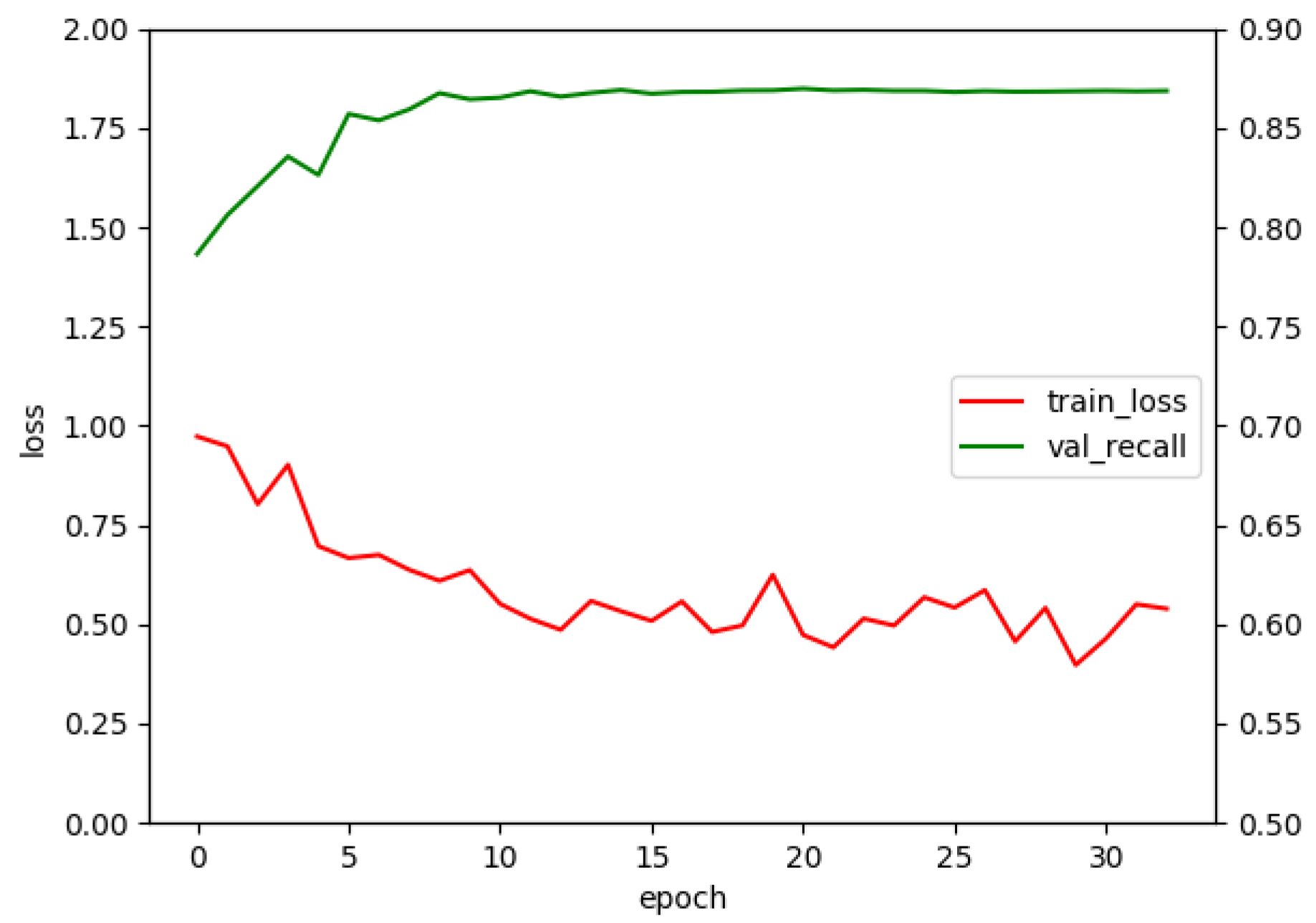
The final model for testing was chosen based on the best recall value in the validation set. The model prediction was counted as accurate when an IOU with the ground-truth box was greater than 0.5 as in the PASCAL VOC challenge [
43]. For the input size, experiments with the image size set to 480 × 270 pixels, and 360 × 203 pixels were conducted. The first resolution achieved a higher recall (86.9% vs. 81.7%). A further increase of accuracy would not allow for real-time processing; which is why the 480 × 270 resolution was used for further experimentation. When the detection module was deployed to a Jetson Tx2, it worked at a speed of 13.7 frames per second (fps). When the SORT tracker, and background subtraction method were added to allow automatic labelling, the whole system worked at a speed of 9.1 fps, which allowed for system deployment. Such a speed allows for the model working in real-time during the automatic labeling stage by processing approximately every third frame. Consequently, for our experiments, every third frame is used only when collecting new samples for the model’s fine-tuning.
Figure 5 shows the training history for the selected model.
Domain adaptation. Even though the trained model performed well on the challenging UA-Detrac dataset, it failed in many seemingly easier cases when tested on the data from our camera (
Figure 6), because CNN-based visual recognition approaches work well only when the test-time conditions are similar to those in the training. Because it is the case domain adaptation methods are needed to improve the performance and, here, we focus on modelling the background, since the camera is static and automatically finds samples for fine-tuning.
To improve the model accuracy, the data were automatically collected for five days, and the model was fine-tuned at the end of each day. Five iterations were chosen, because the self-training procedure is known to provide the best improvements in the initial iterations [
34].
Figure 7 shows some of the automatically labelled samples. 320 images were sampled on average each day. Experiments with a human-in-the-loop scenario were also performed where the task of the human was to filter out images with noisy labels, so, for each image, the human had to only click "accept” or “reject”. It proved to be a very fast procedure, taking 1–2 secs, on average, for each image.
After the labels were collected, they were split into training and validation parts at a ratio of 4:1. During the fine-tuning stage in each epoch, the model was trained on automatically labelled data as well as the same number of randomly selected examples from the UA-Detrac dataset while using the rehearsal technique. The model was validated on the UA-Detrac validation set, and on newly mined data. The model for further testing was chosen by computing a weighted average of the recall on both datasets. In our case, a 9:1 weight ratio was used, because the UA-Detrac dataset is much bigger and those labels contain less noise. One crucial aspect that helped the model to actually work was removing cross-entropy classification from the loss function (Equation (
2)). This was done because the trained model was a relatively poor classifier of the detected vehicles in the deployment environment.
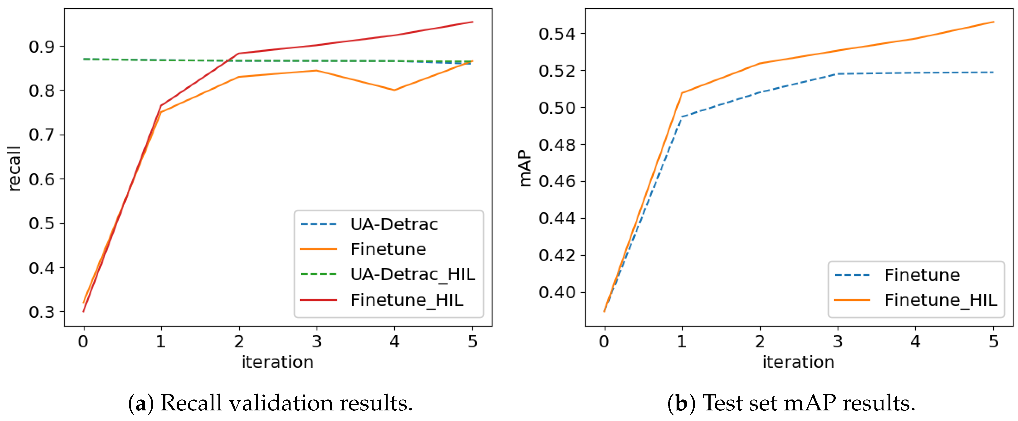
Figure 8a presents validation results after each day.
After the model was fine-tuned for five days, final tests were performed on the data from different days that were manually annotated (
Table 1). There was an increase for each category of vehicles; however, the Others category (which includes mainly trucks) was still not well recognised. Automatic fine-tuning resulted in a relative increase of the mAP (mean average precision) metric by 33% (from 0.39 to 0.519). The mAP is a popular metric in object detection community, and is computed as an area under precision-recall curve. For the human-in-the-loop scenario the mAP score was 0.546 (a 40% relative increase as compared to the baseline scenario). Meanwhile, there was only a slight decrease in the performance for the UA-Detrac dataset (from 87.0% to 86.5%).
Figure 8b shows that the biggest increase was noted in the first timestep. For our fine-tuning technique, the accuracy saturated on the third day, whereas human-in-the-loop scenario still provided a small increase in accuracy on further timesteps.
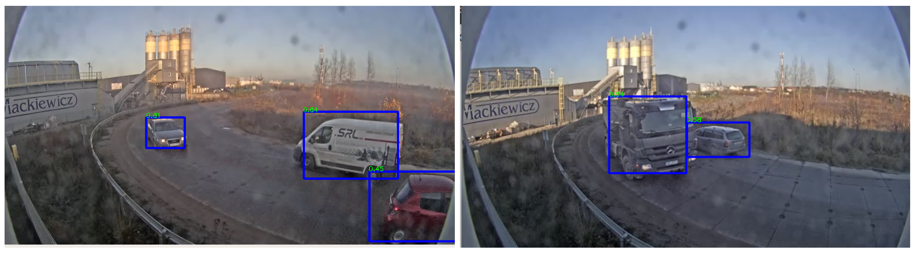
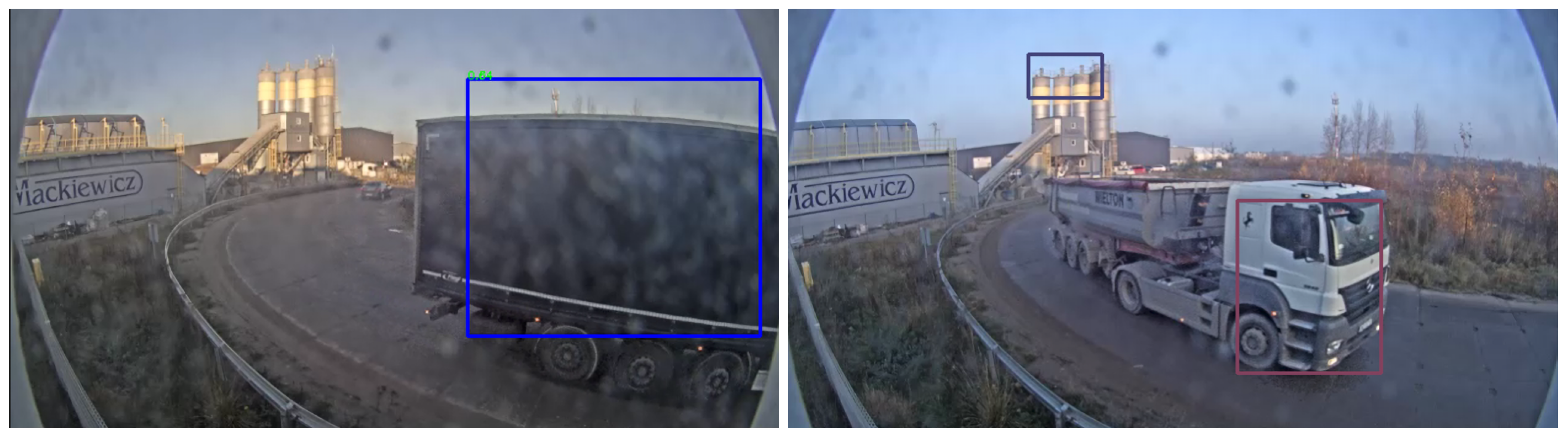
Qualitative results of the improvement are presented in
Figure 9—vehicles were tracked for a longer number of steps because they were much better detected at the the far-end. Such an improvement could be beneficial for increasing the accuracy of speed measurement. Additionally, many of the false-positive detections were removed. It should be noted that trucks are still poorly detected by the fine-tuned detector. That is because the initial detector did not detect trucks well in that environment, which means that automatically discovered examples of trucks were rare, and their labels have been noisy (
Figure 10). As a result, when fine-tuning the model, there was an insufficient amount of labels for trucks to help significantly improve their detection.
Vehicle detection is usually only an intermediate step towards the task of interest, e.g., vehicle counting. To fully evaluate the proposed system, metrics used in multiple-object-tracking (MOT) would also be computed. These include, for example, multiple-object tracking accuracy (MOTA), identification precision (IDP), identity switching (IDSW), and many more [
44]. However, computing those metrics would require annotations of a much higher number of frames. Because of that, in this work, detection accuracy was evaluated. It was shown that the proposed adaptation methods improved the vehicle detection performance and, since the tracking-by-detection paradigm is utilized, a better detection algorithm should lead to better tracking performance. Nevertheless, computing MOT-related metrics remains an important step for future work.
6. Conclusions
In this work, a solution for traffic monitoring was proposed with an unsupervised adaptation, which runs with a speed of 9.1 frames per second on the Jetson Tx2 platform. It was demonstrated that a supervised training application may lead to satisfying vehicle detection performance, even in the case of limited computing power being available. However, a significant drop in accuracy was observed when testing the model on data from our camera, that is, when the test data were from different distribution that the training. This shows that it is very important to test the algorithms in out-of-distribution setting, because, in the real-world, gathering annotated data from deployment environment is not always possible. Nevertheless, we have shown that it is possible to obtain training examples automatically that can be used for further fine-tuning of the model, bringing, in turn, an increase in vehicle detection efficiency when the system is already deployed. The fine-tuned model may improve relative accuracy by 33%. However, it is difficult to design a system that works in a fully autonomous mode, since adding even a small amount of human work in the whole process can significantly improve its performance.
The proposed system consists of many interacting components (for detection, background subtraction, tracking, and labelling), and it requires careful design and testing. The main limitation of the presented method results from the application of a single-stage detector, and a background subtraction algorithm for background modelling. Consequently, the method may not work efficiently in some dense traffic scenes or during the night. This is why detectors that can be trained from sparse labels and a more advanced background modelling technique could bring a further enhancement of the proposed system. In future work, we also plan to test our algorithms on more cameras where the model is fine-tuned on data acquired from several locations at the same time.


